Viability of Feature Detection on Sony Xperia Z3 using OpenCL - Max Danielsson Thomas Sievert
←
→
Page content transcription
If your browser does not render page correctly, please read the page content below
Thesis no: MECS-2015-11

      Viability of Feature Detection on
       Sony Xperia Z3 using OpenCL

                                   Max Danielsson
                                   Thomas Sievert

Faculty of Computing
Blekinge Institute of Technology
SE–371 79 Karlskrona, Sweden
This thesis is submitted to the Department of Computer Science & Engineering at Blekinge
Institute of Technology in partial fulfillment of the requirements for the degree of Master of
Science in Engineering: Game and Software Engineering. The thesis is equivalent to 20 weeks
of full-time studies.

Implementation Source:
https://github.com/autious/harris_
hessian_freak

Contact Information:
Author(s):
Max Danielsson
E-mail: max@autious.net
Internet: http://www.autious.net
Phone: +46 738 21 96 90
Thomas Sievert
E-mail: thomas.t.m.sievert@gmail.com

Externl advisor:
Jim Rasmusson
Sony Mobile Communications

University advisor:
Prof. Håkan Grahn
Dept. Computer Science & Engineering             Internet   :   www.bth.se

Faculty of Computing
Blekinge Institute of Technology                 Phone      : +46 455 38 50 00
SE–371 79 Karlskrona, Sweden                     Fax        : +46 455 38 50 57
Abstract

Context. Embedded platforms GPUs are reaching a level of perfor-
mance comparable to desktop hardware. Therefore it becomes inter-
esting to apply Computer Vision techniques to modern smartphones.
The platform holds different challenges, as energy use and heat gen-
eration can be an issue depending on load distribution on the device.
Objectives. We evaluate the viability of a feature detector and de-
scriptor on the Xperia Z3. Specifically we evaluate the the pair based
on real-time execution, heat generation and performance.
Methods. We implement the feature detection and feature descrip-
tor pair Harris-Hessian/FREAK for GPU execution using OpenCL,
focusing on embedded platforms. We then study the heat generation
of the application, its execution time and compare our method to two
other methods, FAST/BRISK and ORB, to evaluate the vision per-
formance.
Results. Execution time data for the Xperia Z3 and desktop GeForce
GTX660 is presented. Run time temperature values for a run of
nearly an hour are presented with correlating CPU and GPU ac-
tivity. Images containing comparison data for BRISK, ORB and
Harris-Hessian/FREAK is shown with performance data and discus-
sion around notable aspects.
Conclusion. Execution times on Xperia Z3 is deemed insufficient
for real-time applications while desktop execution shows that there is
future potential. Heat generation is not a problem for the implemen-
tation. Implementation improvements are discussed to great length
for future work. Performance comparisons of Harris-Hessian/FREAK
suggest that the solution is very vulnerable to rotation, but superior
in scale variant images. Generally appears suitable for near duplicate
comparisons, delivering much greater number of keypoints. Finally,
insight to OpenCL application development on Android is given.

Keywords: GPU, Feature Detection, Feature Description, Embedded
Device
Acknowledgments

We would like to thank our supervisor Håkan Grahn for being clear, detailed and
  concise with his direction, help and criticism while working on this project.

Additionally we would like to thank our external supervisor Jim Rasmusson for
assisting us with his superior knowledge of the hardware, his invaluable advice,
     and Sony Mobile for the hardware allowing us to develop and perform
                                  experiments.

  Max would like to thank his partner in life, Cilia for being so supportive. I
             probably wouldn’t have gotten this far without you.

                                       ii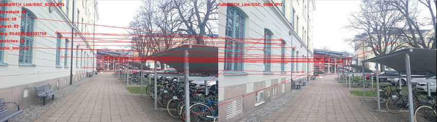
Contents

Abstract                                                                                                                          i

1 Introduction                                                                                                                   1

2 Background and Related Work                                                                                                    4
  2.1 Feature Detection . . . . . . .           .    .   .   .   .   .   .   .   .   .   .   .   .   .   .   .   .   .   .   .   4
  2.2 Feature Description . . . . . .           .    .   .   .   .   .   .   .   .   .   .   .   .   .   .   .   .   .   .   .   5
  2.3 OpenCL . . . . . . . . . . . .            .    .   .   .   .   .   .   .   .   .   .   .   .   .   .   .   .   .   .   .   6
  2.4 OpenCL on the Adreno 330 .                .    .   .   .   .   .   .   .   .   .   .   .   .   .   .   .   .   .   .   .   9

3 Research Questions and Method                                                                                                  11
  3.1 Research Questions . . . . . . . . . . . . . . .                               . . . . . . . .                 .   .   .   11
  3.2 Method . . . . . . . . . . . . . . . . . . . . .                               . . . . . . . .                 .   .   .   12
      3.2.1 Implementation . . . . . . . . . . . . .                                 . . . . . . . .                 .   .   .   12
      3.2.2 Experiment 1: Heat Generation . . . .                                    . . . . . . . .                 .   .   .   12
      3.2.3 Experiment 2: Detector and Descriptor                                    Performance                     .   .   .   12
      3.2.4 Test Image . . . . . . . . . . . . . . .                                 . . . . . . . .                 .   .   .   13
      3.2.5 Comparing Descriptors . . . . . . . . .                                  . . . . . . . .                 .   .   .   13

4 Harris-Hessian Detector                                                                                                        15
  4.1 Convolution in Images .      .   .   .    .    .   .   .   .   .   .   .   .   .   .   .   .   .   .   .   .   .   .   .   15
  4.2 Gaussian Blur . . . . . .    .   .   .    .    .   .   .   .   .   .   .   .   .   .   .   .   .   .   .   .   .   .   .   16
  4.3 Derivative . . . . . . . .   .   .   .    .    .   .   .   .   .   .   .   .   .   .   .   .   .   .   .   .   .   .   .   16
  4.4 Harris Corners . . . . . .   .   .   .    .    .   .   .   .   .   .   .   .   .   .   .   .   .   .   .   .   .   .   .   17
  4.5 Hessian Determinant . .      .   .   .    .    .   .   .   .   .   .   .   .   .   .   .   .   .   .   .   .   .   .   .   18
  4.6 Harris-Hessian . . . . . .   .   .   .    .    .   .   .   .   .   .   .   .   .   .   .   .   .   .   .   .   .   .   .   18
      4.6.1 The Harris Step .      .   .   .    .    .   .   .   .   .   .   .   .   .   .   .   .   .   .   .   .   .   .   .   18
      4.6.2 The Hessian Step       .   .   .    .    .   .   .   .   .   .   .   .   .   .   .   .   .   .   .   .   .   .   .   19

5 FREAK Descriptor                                                                                                               20
  5.1 Binary Descriptors . . . . . . . . . . . . . . . . . . . . . . . . . .                                                     20
  5.2 FREAK . . . . . . . . . . . . . . . . . . . . . . . . . . . . . . . .                                                      20

                                               iii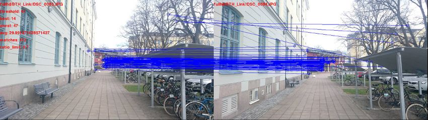
6 Implementation                                                                                                                22
  6.1 Data Representation . .      .   .   .    .   .   .   .   .   .   .   .   .   .   .   .   .   .   .   .   .   .   .   .   22
  6.2 Algorithm Overview . .       .   .   .    .   .   .   .   .   .   .   .   .   .   .   .   .   .   .   .   .   .   .   .   23
  6.3 Harris-Hessian . . . . . .   .   .   .    .   .   .   .   .   .   .   .   .   .   .   .   .   .   .   .   .   .   .   .   25
      6.3.1 Prefetching . . .      .   .   .    .   .   .   .   .   .   .   .   .   .   .   .   .   .   .   .   .   .   .   .   27
      6.3.2 Work Group Size        .   .   .    .   .   .   .   .   .   .   .   .   .   .   .   .   .   .   .   .   .   .   .   28
  6.4 FREAK . . . . . . . . .      .   .   .    .   .   .   .   .   .   .   .   .   .   .   .   .   .   .   .   .   .   .   .   28

7 Experimental Results                                                                                                          30
  7.1 Program Execution Times . . .                 .   .   .   .   .   .   .   .   .   .   .   .   .   .   .   .   .   .   .   30
      7.1.1 Prefetching Effects . . .               .   .   .   .   .   .   .   .   .   .   .   .   .   .   .   .   .   .   .   31
      7.1.2 Workgroup Size Results                  .   .   .   .   .   .   .   .   .   .   .   .   .   .   .   .   .   .   .   32
  7.2 Temperature . . . . . . . . . . .             .   .   .   .   .   .   .   .   .   .   .   .   .   .   .   .   .   .   .   33
  7.3 Performance . . . . . . . . . . .             .   .   .   .   .   .   .   .   .   .   .   .   .   .   .   .   .   .   .   37

8 Discussion                                                                                                                    43
  8.1 ALU Memory Ratios and Caching . . . . .                               .   .   .   .   .   .   .   .   .   .   .   .   .   43
  8.2 Possible Optimizations . . . . . . . . . . .                          .   .   .   .   .   .   .   .   .   .   .   .   .   44
      8.2.1 Using Texture Samplers . . . . . .                              .   .   .   .   .   .   .   .   .   .   .   .   .   44
      8.2.2 Half Floats . . . . . . . . . . . . .                           .   .   .   .   .   .   .   .   .   .   .   .   .   45
      8.2.3 Gaussian Blur . . . . . . . . . . . .                           .   .   .   .   .   .   .   .   .   .   .   .   .   46
  8.3 The Use of GPUs on Embedded Platforms                                 .   .   .   .   .   .   .   .   .   .   .   .   .   46
      8.3.1 OpenCL on Android . . . . . . . .                               .   .   .   .   .   .   .   .   .   .   .   .   .   47
      8.3.2 Screen Lag . . . . . . . . . . . . . .                          .   .   .   .   .   .   .   .   .   .   .   .   .   47
      8.3.3 Working in OpenCL . . . . . . . .                               .   .   .   .   .   .   .   .   .   .   .   .   .   47

9 Conclusions and Future Work                                                                                                   49
  9.1 Heat Generation Properties . . . . . . . . . . . . . . . . . . . . .                                                      49
  9.2 Matching performance . . . . . . . . . . . . . . . . . . . . . . . .                                                      49
  9.3 Practical Viability of Implementation . . . . . . . . . . . . . . . .                                                     50

Appendices                                                                                                                      54

A Appendix A                                                                                                                    55

                                               iv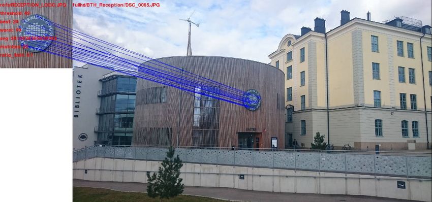
List of Figures

2.1   Visual example of SIMD execution. The rows are linear arrays
      of data, each column is executed in a separate task allowing for
      parallelization. . . . . . . . . . . . . . . . . . . . . . . . . . . . . .   7
2.2   Work groups are multi-dimensional. In this example each work
      group is two-dimensional and consist of 32 tasks each. There are
      nine work groups in the image resulting in a total of 288 individual
      tasks. . . . . . . . . . . . . . . . . . . . . . . . . . . . . . . . . . .    7
2.3   OpenCL memory locality visualized. Global memory is accessible
      from all four work groups while local memory is only available
      within a single work group and private memory is limited to a
      single running task. . . . . . . . . . . . . . . . . . . . . . . . . . .     8
2.4   Memory locality visualization specific to the Adreno 330. Global
      memory is accessible from all four shader processors while local
      memory is only available within a single shader processor and pri-
      vate memory is limited to a single running task running on an
      ALU. The unified L2 cache is used for all types of memory, but the
      L1 cache is reserved for texture images. . . . . . . . . . . . . . . .        9

3.1   Our chosen test image featuring a series of posters, original image
      has a resolution of 800x600. . . . . . . . . . . . . . . . . . . . . .       13

4.1   A nine element box filter applied on the value in the middle. . . .          16
4.2   A demonstration of some of the steps in the Harris algorithm. From
      left to right: Input image, Gaussian blur, derivative along the y
      axis, Harris corner response (before non-max suppression). Origi-
      nal image By POV-Ray (Rendered in POV-Ray by user:ed_g2s.)
      [CC BY-SA 3.0 (http://creativecommons.org/licenses/by-sa/3.0)],
      via Wikimedia Commons. . . . . . . . . . . . . . . . . . . . . . .           18

                                        v
6.1   Visual representation of the algorithm. On the left side is the host
      CPU with initialization of data, summing of keypoints counts and
      execution of FREAK. On the right is the twelve executional kernel
      calls to perform Harris-Hessian for a given scale and finally the
      keypoint generation kernel call which gathers the resulting data.
      Order of execution is from top to bottom. . . . . . . . . . . . . .       24
6.2   Data flow in Harris-Hessian. Solid boxes indicate kernel executions
      and the dotted boxes are buffers or data. Green boxes are input
      and orange are the resulting output for a given sigma. Red boxes
      are the results sent to the descriptor. The larger dotted border in-
      dicates sigma iteration, anything within this border is re-performed
      for each sigma. . . . . . . . . . . . . . . . . . . . . . . . . . . . .   26
6.3   Standard gather algorithm. Data is incremented atomically at the
      target memory location which prevents data races but adds extra
      synchronization between tasks. . . . . . . . . . . . . . . . . . . .      27
6.4   The memory access of an individual task compared to the entire
      work group on a two dimensional image. By utilizing local memory
      it is possible to remove overlapping global memory accesses. . . .        28

7.1   Execution times on Xperia Z3 for individual kernels and on FREAK,
      named ”build descriptor”, values are from the median of 10 runs. .        30
7.2   Execution times on a PC with an Intel i5 and GTX 660 for in-
      dividual kernels and on FREAK, named ”build descriptor”, values
      are from the median of 10 runs. . . . . . . . . . . . . . . . . . . .     31
7.3   Graph detailing the performance of prefetching and direct global
      access in Gaussian blur kernels. The data is obtained by running
      the program 10 times and then taking the median value of each
      sigma, using the average is similar with some stronger variations
      due to occasional errors in the OpenCL device timers which re-
      sulted in values being reported as near zero. . . . . . . . . . . . .     32
7.4   Graphs detailing the different run times for Gaussian blur on the
      Xperia Z3 for different work group sizes. Values are averaged from
      10 runs for each work group size. Outlier extreme values were
      removed before average as they skewed the results. . . . . . . . .        33
7.5   Graphs describing the heat over the duration of 3500 seconds, from
      start of idle phone. The two smaller graphs show a detailed view
      of the beginning and end of the program to give a clear contrast. .       34
7.6   Graphs describing the CPUs frequency through the duration of
      the heat stress test. The two smaller graphs show the beginning
      and end of the test, to contrast that the value variations appear
      unchanged. In the graphs we see that CPU 1 and CPU 4 both are
      active while CPU 2 and 3 appear inactive. . . . . . . . . . . . . .       35

                                      vi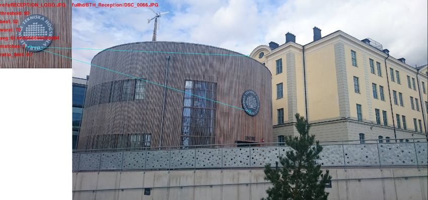
7.7 Graphs describing the GPU activity through the duration of the
heat stress test. The two smaller graphs show detailed information
in the beginning and end of the test. The graphs indicate that
the GPU is active with occasional dips and there appears to be no
variation between beginning and end of the test. . . . . . . . . . . 36
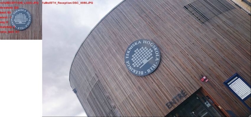
7.8 Near-duplicate images of buildings. The distribution of points in-
dicate that Harris-Hessian/FREAK is more scale invariant than its
competitors. . . . . . . . . . . . . . . . . . . . . . . . . . . . . . . 38
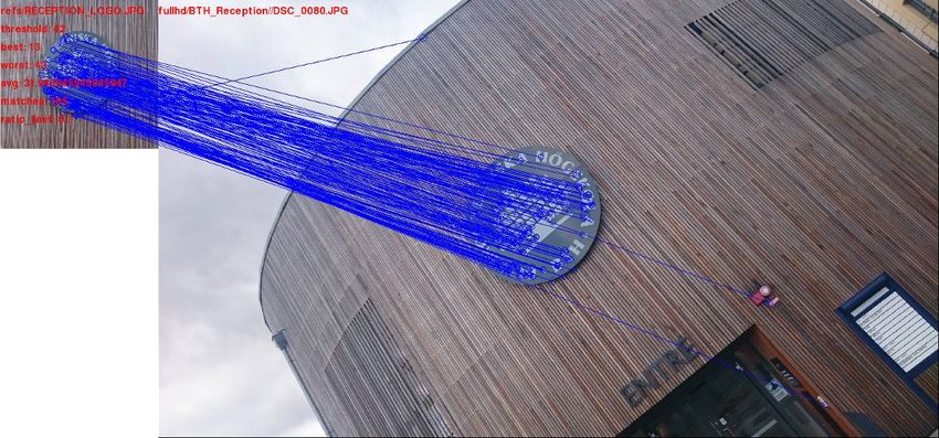
7.9 Reference comparison of a logotype with a slight viewpoint change.
With no rotation, ORB and Harris-Hessian/FREAK perform sim-
ilarly. . . . . . . . . . . . . . . . . . . . . . . . . . . . . . . . . . . 39
7.10 Reference comparison of a logotype with a more drastic viewpoint
change. This results in none of the algorithms being able to find
matches. . . . . . . . . . . . . . . . . . . . . . . . . . . . . . . . . 40
7.11 Reference comparison of a logotype with rotation. Apparently
ORB’s rotational invariance performs much better in this case,
as neither of its competitors manage to find matches. . . . . . . . 41
7.12 Reference comparison of a poster with scale change. While ORB
is not guaranteed to handle scale change very well, it is still the
strongest alternative here, by far. . . . . . . . . . . . . . . . . . . 42
vii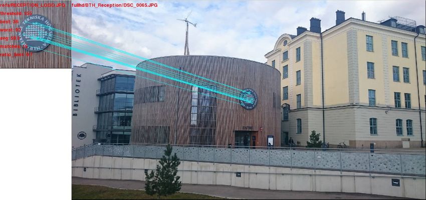
Chapter 1
                                                           Introduction

Digital images today play a large role in how we communicate with each other. As
modern-day cellphones are often equipped with digital cameras, the availability
of taking a photograph has increased. Likewise the applications of Computer
Vision (CV) have become more numerous, and with the increasing computational
power of computers and cellphones so has their availability. Feature detection is
a fundamental part of CV used to discover abstract features, which can later be
used for a multitude of purposes. As such, implementing feature detection on a
heterogeneous device such as a smartphone is a relevant topic of research.
     Modern embedded systems have become quite powerful. The Qualcomm
Snapdragon 800 is a heterogeneous device, commonly used in cellphones such
as the Xperia Z3, which contains a quad-core ARMv7 Central Processing Unit
(CPU), a 128 core Adreno 330 Graphics Processing Unit (GPU) and a Hexagon 3
threaded Digital Signal Processor (DSP). Each processor has different properties;
the GPU promises an extremely high throughput thanks to massive paralleliza-
tion but has a simple ALU design compared to the CPU, which aims to maximize
performance per thread, whereas the DSP, instead, is designed with high energy
efficiency in mind. The consequence is that a single CPU core is vastly more
complicated than a GPU core and therefore die utilization limits the core count
to a much lower number. This also means that a CPU uses more energy per core.
     GPUs boast a much higher FLOPS (Floating Point Operations per Second)
measure than CPUs and research shows that it is possible to save energy in most
modern systems by implementing certain algorithms on the GPU rather than the
CPU [21]. The challenge in achieving a high utilization lies in designing algo-
rithms that are adapted to the GPU’s architecture, which is considered harder to
do. It has been shown that a well designed GPU algorithm can outperform a CPU
implementation for certain applications[4], but there is a clear gap in required ex-
perience and competence between the two as single threaded programming is well
known while many-core programming is a relatively unexplored concept.
     The Snapdragon 800, much like similar platforms, generates a large amount
of heat when all units are running on full frequency, making the experience for
the user problematic and lowering the lifespan of the hardware. The problem can
be partially solved from software by lowering the clock of the hardware or turning

                                         1
Chapter 1. Introduction 2
off units. By running units in intervals or "bursts" it is possible to keep the heat
of the unit low while still trying to achieve good enough performance for the user
experience.
As mobile hardware gets more powerful, more complex techniques can be
employed. An obvious field of application for modern smartphones is computer
vision, since cameras are part of their core feature set. Furthermore, as processing
of images by their nature tends to consist of many similar, parallel tasks, such
algorithms are advantageously performed on the GPU[22].
In our work we focus on building a feature detector and feature descriptor pair
(details in Chapter 2). One of our goals is to find and implement an algorithm
that is suitable for the embedded environment. With this in mind we have chosen
Harris-Hessian[23] as a detector and FREAK[1] as our descriptor. Harris-Hessian
was chosen because it is an algorithm specifically designed for a GPU and proven
to perform well in such an environment. We focus on a detector implemented
on the GPU as the task is computationally intensive and generally parallelizable
making it more suitable for GPU execution than CPU execution. FREAK was
chosen because of its fast matching speeds and simple implementation, which is
relevant for a platform with limited computational ability.
After building our implementation of what we call Harris-Hessian/FREAK we
run the application in full force to observe the heat generation characteristics of
the program, and will adapt the program to allow it to run without overheating
the device. In our work we will also pay attention the execution time to see
what scope the application might have in practice, and compare it to the same
implementation running on a conventional desktop Nvidia GeForce GTX660 card
hosted by an i5 CPU. The hardware was chosen primarily because of its availabil-
ity to us. It is, however, a very common middle end card, making our comparison
accessible to a wide audience. Comparing a desktop setup with the embedded
device will give us and others a chance at a better understanding of the Adreno
330’s function and limitations by having a comparison to well known hardware,
as Qualcomm1 is secretive with some of the details of theirs.
Our motivation for building a combined detector and descriptor solution is
largely driven by the interests of Sony Mobile, who wish to get a greater under-
standing of the capabilities of their device. The use and focus on the Xperia Z3
and using OpenCL[17] for GPU programming is chosen by request from Sony.
To our knowledge, Harris-Hessian and FREAK is a novel combination within
the scientific field, and so, to get an understanding of its functional performance
we intend to compare it with two other well studied descriptor and detector
pairs: ORB and FAST/BRISK. The study will consist of a selection of images
that we consider interesting in presenting the strengths and weaknesses of Harris-
Hessian/FREAK, ORB and BRISK, and discuss what it might mean in an appli-
1
Qualcomm is the hardware developer of the Snapdragon 800 and Adreno 330 hardware
series. They are one of the largest developers of embedded systems for the cellphone market.Chapter 1. Introduction 3
cation. Additionally our contribution will be a fully functional implementation
released under the BSD license, links to source can be found in the cover pages.
The rest of this thesis is structured as follows:
Chapter 2 presents a summary of the background and related work.
Chapter 3 presents the research questions and their motivations as well as the
method with which we intend to answer them.
Chapter 4 presents a summary of the Harris-Hessian algorithm proposed by Xie
et al.
Chapter 5 similarly presents a summary of the FREAK algorithm proposed by
Alahi et al.
Chapter 6 presents an explanation of our implementation of the detector and
descriptor.
Chapter 7 presents the and discusses the results of the experiments run.
Chapter 8 presents the conclusions made and proposed future work.Chapter 2
Background and Related Work
The study on how to interpret digital images is commonly referred to as Com-
puter Vision. This is a wide field with applications including for example object
recognition, image restoration and scene reconstruction. The aim of CV is to
extract abstract information from an image, and these applications are used in
a wide variety of fields, such as industrial automation, medical image analysis,
geo-location for unmanned vehicles, and others.
2.1 Feature Detection
Within the field computer vision, feature detection refers to methods of trying to
locate arbitrary features that can afterwards be described and compared.
In 1988 Harris and Stephens proposed an operator to measure the "corner-
ness" of a point in an image[9]. Their measure is an improvement of Moravec’s
detector[16], and detects corners as well as edges using differential operators
to estimate their direction. However, Harris corners are not scale-invariant.
Mikolajczyk and Schmid aimed to remedy this by detecting corners at succes-
sively larger scales and choosing a "characteristic scale" where the Laplacian-of-
Gaussian (LoG) reaches a maximum[15].
Lowe proposed in 1999 a Scale-Invariant Feature Transform (SIFT). SIFT has
since become somewhat of an industry standard. It includes both detector and
descriptor. Its detector is based on calculating a Difference of Gaussians (DoG)
with several scale spaces. It can be shown that the DoG is very similar to the
LoG, but it is significantly cheaper computationally[13].
Partially inspired by SIFT, Bay et al. proposed their detector Speeded-Up
Robust Features (SURF)[2] in 2006. The aim of SURF is mainly - as the name
hints - to speed up the detection (and description) while still maintaining high
performance. To achieve this Bay et al. make use of integral images and Hessian
determinants. SURF and SIFT are often used as base lines in evaluations of
other detectors. Note that in this thesis "performance" refers to the quality of
the results from a detector and descriptor pair, not execution speeds.
The detector chosen for our experiments was proposed in 2010 by Xie et al.
and is inspired by Mikolajczyk and Schmid, particularly their use of a multi-scale
4Chapter 2. Background and Related Work 5
Harris operator[23][15]. However, instead of increasing the scale incrementally,
they examined a large set of pictures to determine which scales should be evalu-
ated so that as many features as possible only are discovered in one scale each.
This resulted in nine pre-selected scales and two additional ones around the one
deemed to be closest to the picture’s characteristic scale. After finding features
this way, Xie et al. propose culling weak corners using the Hessian determinant.
As the fundamental operators in this detector are the Harris operator and the
Hessian determinant, it is dubbed the "Harris-Hessian detector". It is important
to note that Xie et al. designed this detector specifically to be implemented on
the GPU, which makes it suitable for this thesis.
In 2005 Rosten et al. proposed a detector based on a different idea. To reach
a low execution time they choose to simply sample points on a circle surrounding
the examined pixel and compare their intensities. If enough differ, the algorithm
is said to have found an interest point. This detector is called Features from
Accelerated Segment Test (FAST)[19].
2.2 Feature Description
Detecting a feature is merely half the work. In order for the information provided
by a detector to be useful, it needs to be described in such a manner that the
same feature in a different image can be compared and confirmed to be matching.
What is typically done is some sort of evaluation of the image around the chosen
keypoint, which is then compiled into a vector (called a descriptor) that can be
compared using a vector norm.
SIFT, SURF, and traditionally many other descriptors use strategies that are
in some form variations of histograms of gradients (HOG). What this means is
that for a keypoint in an image, an area around the point (its size decided by the
scale of the keypoint) is divided into a grid. Each cell of the grid is subdivided
into a smaller grid, and in each sub-cell, a gradient is computed. The orientations
of the gradients are rounded, and a histogram of the gradients’ rotations and ori-
entations is made for each cell. These histogram typically make up the descriptor.
Note that this is a rough explanation of HOG-based descriptors. SURF, while
based on the same principle, uses Haar wavelets instead of gradients to speed up
computation. The resulting descriptors are vectors of a high dimension (usually
at least 128) which can be compared using for example Euclidean distance.
In 2010 Calonder et al. proposed a new type of descriptor called Binary Robust
Independent Elementary Features (BRIEF)[5]. Instead of using HOGs, BRIEF
samples a pair of points at a time around the keypoint, then compares their
respective intensities. The result is a simple one or zero concatenated into a string,
which suggests the categorization "binary descriptor" being coined. Calonder
et al. do not propose a single sampling pattern, rather they consider five different
ones. The resulting descriptor is nevertheless a binary string. The benefits ofChapter 2. Background and Related Work 6
binary descriptors are mainly that they are computationally cheap, as well as
suitable for comparison using Hamming distance[8], which can be implemented
effectively using the XOR operation.
Further work into improving the sampling pattern of a binary descriptor has
been made, most notably Oriented FAST and Rotated BRIEF (ORB)[20], Bi-
nary Robust Invariant Scalable Keypoints (BRISK)[12], and Fast Retina Key-
point (FREAK)[1]. The descriptor we choose to implement for the purpose of
this thesis is FREAK, in which machine learning has been employed to find a
sampling pattern that requires potentially fewer comparisons than the previously
proposed binary descriptors. An interesting property of FREAK is that the re-
sulting sampling pattern is similar to saccades, which is what the human eye
does when observing. FREAK also generates an hierarchical descriptor allowing
for early out comparison. As FREAK severely reduces the number of necessary
operations when comparing, it is suitable for a mobile implementation aimed to
generate as little heat as possible.
2.3 OpenCL
OpenCL1 is an open framework for executing programs on heterogeneous com-
puters, its model is well suited for execution of programs on GPUs. It is very
similar to the Nvidia specific CUDA framework. OpenCL consists of a standard
C[11] library for communication between devices and a C99 based language for
writing programs. An OpenCL program is referred to as a kernel. Each kernel
can, similarly to a normal C-function, take arguments of data or pointers.[17]
The standard paradigm of OpenCL programming is to split a program into
smaller tasks, commonly this split is a separation of data and not program mean-
ing that each task runs the same program with the only difference being some or
all of the input. This makes OpenCL suitable for what is called stream process-
ing, a paradigm where a large array of data has its individual elements divided
to different tasks, see Figure 2.1.
It is possible to share memory between tasks, but it complicates program-
ming in that it might require synchronization, primarily on read-after-write or
write-after-write situations, where one task reads the memory that one or more
other tasks might write to first. Such synchronization is usually expensive, not
only because it invokes a dependency making tasks wait for each other, but also
because synchronization units often require extra communication with globally
synchronized memory which can be costly[7].
Tasks are grouped into what is called a work group. A work group is multi-
dimensional unit of tasks. An execution of a kernel is run using one or more work
groups, see Figure 2.2.
1
Offical webpage of the OpenCL standard: https://www.khronos.org.Chapter 2. Background and Related Work 7
Task
src1
src2
dest
1 2 3 4 5 n
Figure 2.1: Visual example of SIMD execution. The rows are linear arrays of
data, each column is executed in a separate task allowing for parallelization.
Tasks
WG
WG 12
WG 4
Work Group Size
8
Global Size
24
Figure 2.2: Work groups are multi-dimensional. In this example each work group
is two-dimensional and consist of 32 tasks each. There are nine work groups in
the image resulting in a total of 288 individual tasks.
In OpenCL there are four types of memory; global, constant, local and private,
see Figure 2.3. Global memory is accessible to all tasks and the host of the
program. Generally global memory resides on the device RAM and is the slowest
to access for a task. Constant memory follows the same rules as global, but is
a read only memory from the perspective of the device. Constant memory is
commonly stored in RAM, but is easier to cache from a hardware perspective
and is therefore likely to have faster access times. Local memory is shared within
a work group and is often stored in a special memory bank tied to units handling
the work groups. Finally, private memory is limited to a single task and is often
stored in a register-like memory.
Programs written in OpenCL C are similar to C programs but differ in some
important aspects. By declaring a function with the keyword kernel it is made
available to call from the host through the OpenCL API, in Listing 2.1 we
demonstrate a simple kernel which calculates an X axis Gaussian blur on a two-
dimensional image. The first parameter is the filter, which is stored in global
memory, second is the size of the filter, as it varies depending on the sigma, thirdChapter 2. Background and Related Work 8
Local
Global
WG WG WG WG Constant
Task Task Task Task
Private
Task Task Task Task
Task Task Task Task
Task Task Task Task
Figure 2.3: OpenCL memory locality visualized. Global memory is accessible
from all four work groups while local memory is only available within a single
work group and private memory is limited to a single running task.
is input data buffer and fourth is the resulting output buffer. When running the
program each task is assigned a globally unique ID. The globally unique ID maps
to the span of the execution call and the span matches the size of the buffer in
our example. That means that we run a task for each pixel. The ID is requested
using the get_global_id function. To create a frame of reference, if we were to
make this function sequential for execution on a single core machine we would
simply create a 2D loop for the int2 coord value.
kernel void gaussx (
global float * gauss_kernel ,
int kernel_radius ,
global float * input ,
global float * output ,
int width )
{
int2 coord = ( int2 )( get_global_id (0) , get_global_id (1));
hh_float sum = 0;
for ( int i = - kernel_radius ; iChapter 2. Background and Related Work 9
2.4 OpenCL on the Adreno 330
OpenCL is a relatively generic standard and is not limited to graphics card hard-
ware. The standard, however, is designed to accommodate such hardware quite
well.
The different classes of memory in the OpenCL standard allow devices to
perform some memory type specific optimizations that would be impossible oth-
erwise, such as a simplified cache for constant memory.
Global memory is the slowest type of memory on most GPUs, and in the case
of Adreno 330 it is likely to be a difference of an order of magnitude between
global and local memory. We cannot be completely sure this is the case for the
Adreno 330, but it is what is reported for the Nvidia series cards[10]. We consider
it reasonable to act under the assumption that a similar restriction applies to the
Adreno 330.
Global
Constant
Local
SP SP SP SP
ALU ALU ALU ALU Private
ALU ALU ALU ALU
ALU ALU ALU ALU
ALU ALU ALU ALU
Figure 2.4: Memory locality visualization specific to the Adreno 330. Global
memory is accessible from all four shader processors while local memory is only
available within a single shader processor and private memory is limited to a
single running task running on an ALU. The unified L2 cache is used for all types
of memory, but the L1 cache is reserved for texture images.
The Adreno 330 has 4 shader processors (SP) and a total of 128 arithmetic
logic units (ALUs), divided evenly, each SP has 32 ALUs each. Every SP has its
own local memory. Mapping the Adreno to OpenCL, a work group can at most
exist inside of a single SP meaning that the optimal work group size should beChapter 2. Background and Related Work 10
roughly 32 tasks in most cases, of course this also depends on other factors such
as local memory usage.
Based on documentation[18] it appears that the Adreno 330 does not treat
constant memory differently than normal buffer memory, meaning that they are
both cached in the L2 cache. Image data memory appears to have an extra L1
cache, closer to the SP, see Figure 2.4.Chapter 3
Research Questions and Method
This thesis concerns implementing and exploring the properties of a feature detec-
tor and descriptor on Sony’s Xperia Z3. The agenda is to find a viable combination
of algorithms for real-time use on the hardware.
3.1 Research Questions
1. What are the heat properties of GPU execution on the Xperia Z3?
Insight into how the system’s temperature is affected by execution of
an algorithm is crucial to understand its range of applications. What
we are looking for is an execution configuration that does not cause
the phone to overheat.
To answer this question we run an experiment where we continuously
execute the implemented algorithm while measuring temperature, to
try and force the unit to lower its frequency or shut down. If necessary,
we further explore configurations where the algorithm is executed in
bursts, to explore the cooling properties of the unit.
2. How does the combination of Harris-Hessian and FREAK compare
with FAST/BRISK and ORB?
The Harris-Hessian detector coupled with the FREAK descriptor is
an untried combination. To verify that it is a worthwhile endeavour,
a comparison with existing approaches is called for.
To answer this question we compare the number of matches made with
the different algorithms. We monitor the number of matches made
while increasing the Hamming distance threshold, and we manually
note when false matches start appearing.
11Chapter 3. Research Questions and Method 12
3.2 Method
We run two experiments, intended to answer one research question each. The
first one concerns the heat properties of the Xperia Z3, and the second concerns
the performance1 of Harris-Hessian and FREAK, compared to contemporary al-
ternatives. We consider the implementation2 of the Harris-Hessian detector as an
additional result, since to our knowledge no source code or implementation has
been made public by the authors. We will also run some execution times tests on
the implementation to give an idea of its application.
3.2.1 Implementation
As Xie et al. provide no implementation details of the Harris-Hessian detector, a
significant portion of this thesis is concerned with this task. We first fashion a
sequential implementation on the CPU, to use as reference and validation when
developing the parallel GPU implementation. While we also implement FREAK
to work in combination with Harris-Hessian. Much of the code for FREAK is
taken directly from Alahi et al.’s original, open source implementation. We will
perform execution time test on the full implementation and the run time on the
Xperia Z3 with a desktop computer running a GTX660 and Intel i5. We will also
provide an analysis of the implementation, detailing the strengths, weaknesses
and future work.
3.2.2 Experiment 1: Heat Generation
For the first experiment, we let the Xperia Z3 execute Harris-Hessian and FREAK
on an image indefinitely, while tracking temperature on the chip and clock fre-
quency of the processing units. Provided that the temperature gets too high, the
phone will clock down or shut down. If we can achieve this, we introduce pauses
in the running of the implementation to reach a level where the system does not
overheat.
3.2.3 Experiment 2: Detector and Descriptor Performance
In the second experiment we use Harris-Hessian/FREAK, ORB, and FAST/BRISK
on a set of images, then perform matching using Hamming distance. We addition-
ally employ a ratio test which evaluates the ratio between the two smallest match
distances and discards any match where it is greater than a given threshold. This
test concludes that if two matches are too similar, they are not unique enough to
be meaningful and as such removes false matches. The proper magnitude of this
1
Note that "performance" in this instance refers to some sort of qualitative measure of the
results of the algorithm, not its execution speed.
2
Source link is available on the cover pages.Chapter 3. Research Questions and Method 13 threshold varies with the use case. For our experiment we choose a fixed value of 0.7 with the purpose of minimizing the amount of false matches. In the results we present a selection of images we feel highlight the different characteristics of the compared algorithms. We show the amount of matches made as a function of the distance between the keypoints, and highlight up to the three first false matches for each algorithm. Additionally we present the total number of matches made at a distance threshold where a maximum of three false matches has been discovered. 3.2.4 Test Image All execution time tests where performed using the image shown in Figure 3.1. Image content does not affect Harris-Hessian algorithms significantly, but can have a major impact on the FREAK algorithm. The reason for this is that different images inherently have a different number of keypoints and the FREAK implementation scales linearly with the number of descriptors. There are also no limitations implemented in how many descriptors are encoded, something that would be very relevant in a final implementation as it does not only effect the execution time, but storage requirements for the descriptor. Figure 3.1: Our chosen test image featuring a series of posters, original image has a resolution of 800x600. 3.2.5 Comparing Descriptors Description comparison is done on the resulting data. The FREAK data for two images is naively compared one-to-one using the Hamming distance[8] which in the case of binary strings - the output of FREAK - can be simplified into a bit-wise XOR operation and bit counting. The computational complexity of the naive solution is O(m · n) where m and n is the number of keypoints in each
Chapter 3. Research Questions and Method                                          14

respective image, meaning that computational growth is quadratic for equal-sized
and equally complicated images.
    When comparing descriptors the best match is evaluated for final utility. It
common to apply a threshold value, setting a minimum distance between key-
points for a valid match. Another common filter, used by for example Alahi et al.,
is to calculate the ratio between distance of the best and second best match, the
value indicates how unique a match is, this ratio is calculated as r = s/b where r is
the ratio, s is the second best match and b is the best. A low ratio indicates that
the keypoints is unique. What threshold to use is very application specific and
varies between cases. It is possible to develop heuristics to dynamically calculate
suitable values but that is out of the scope for this paper.
Chapter 4
Harris-Hessian Detector
The detector consists of two steps: Discovering Harris corners using the Harris-
affine-like detector on nine pre-selected scales as well as two additional scales
surrounding the most populated one, then culling weak points using a measure
derived from the Hessian determinant. What follows is a brief explanation of
the basic mathematical operators used in the algorithm, then an overview of how
they are put together.
4.1 Convolution in Images
Convolution is an essential operation in image processing. In the general case it
is defined as Z ∞
(f ∗ g)(t) f (τ )g(t − τ )dτ
−∞
where f and g are functions. Typically, in signal processing one talks about a
signal and a kernel or filter (f and g, respectively, in this case). Usually the filter
is only non-zero for a finite interval. In the discrete case of image processing,
applying a filter to an image boils down to sampling an area around each pixels,
and summing the values multiplied by weights found in the filter. For example,
the filter
( 13 13 13 )
applied to a pixel p(x) where x is its horizontal position in the image will sum a
third of p(x − 1), p(x) and p(x + 1) to a pixel p0 (x) in the output image. This
particular filter will produce a uniform, horizontal blur. A filter can just as easily
be of two dimensions. In the case of the uniform blur, it would result in a box
filter: 1 1 1
9 9 9
1 1 1
9 9 9
1 1 1
9 9 9
and an intuition to its application can be seen in Figure 4.1. The Harris-Hessian
detector features two kinds of kernels that will be explained in the sections that
follow; the Gaussian blur and the derivative filters.
15Chapter 4. Harris-Hessian Detector 16
2+8+6+1+9+5+3+4+7
=5
9
2 8 6
1 9 5 5
3 4 7
Figure 4.1: A nine element box filter applied on the value in the middle.
4.2 Gaussian Blur
A Gaussian blur effect is achieved when convolving a signal with the Gaussian
function:
1 x2
G(x) = √ e− 2σ2
2πσ 2
Where x is the distance from the center point of blurring. This filter is a blur
based on weighted sums derived from normal distribution, which will yield a
more accurate representation than a box filter. A very important aspect of the
Gaussian blur is that it is a low-pass filter, meaning the filter removes noise that
could generate artifacts when applying other kernels. The usage of a Gaussian
filter in feature detection is intuitive; given e.g. a grainy image, one wants to
avoid that such "grains" become classified as corners or features.
In two dimensions, the Gaussian filter distributes the weights of surrounding
pixels in a circular pattern - the further away a pixel is from the center of the
blur, the smaller the contribution to the output pixel. By contrast, the box filter
instead assigns equal contribution to every pixel inside a specified rectangle. The
size of the Gaussian’s "sampling circle" depends on the σ factor; the circle’s radius
r = 3σ. This proportionality has a serious implication on the computational cost
of the Gaussian filter for large σ, i.e. heavy blurring.
4.3 Derivative
The derivative operator describes how much a function is changing in a given
point. If one regards an image I as a function of its coordinates x, y, one can
apply a derivative filter to highlight the places where change is high, e.g. edges and
corners. However the derivative is a one-dimensional operation, so one typically
uses two separate filters:
−1
∂ ∂
= ( −1 0 1 ), = 0
dx dy
1
which calculate the derivatives in the x and y directions, respectively. As the
derivative is originally a continuous operation examining the direction over an
infinitesimally small ∆, the above kernels are naturally discrete approximations.
To make the approximations more accurate and resistant to noise in the image,Chapter 4. Harris-Hessian Detector 17
one typically applies a smoothing filter, such as the Gaussian. As this procedure
is so common, it is named the "Gaussian derivative".
4.4 Harris Corners
Moravec defines a corner in an image to be a point with low self-similarity[16], i.e.
a point whose surrounding points all differ from it. His detector suffers from not
being isotropic (invariant to rotation), which Harris and Stephens proposed to
remedy with their measure of auto-correlation, also called Harris corner response.
The Harris corner response is calculated by examining the summed squared differ-
ences between a pixel and its surrounding pixels. In which area the neighbouring
pixels are to be examined is defined by a window function, w(x, y). To produce
isotropic corners, the area of the window needs to be circular. A circular sampling
filter commonly used in image processing is the Gaussian blur. Approximating
sums of squared differences using its Taylor series approximation yields the Harris
matrix: 2
hIx i hIx Iy i
2
M = σD
hIx Iy i hIy2 i
Where Ii is the partial Gaussian derivative (with σ = σD ) of a pixel in the image
at a given point in the i direction. The angled brackets denote the summation of
all elements within the window function, which in this case is a Gaussian kernel
with σ = σI . Thus, to extract Harris corners at a given scale - window size -
two Gaussian filters are applied; one during derivation and one during the final
summation, called integration. Typically the σD used in derivation is slightly
smaller than the integration scale σI , to remove noise of relevant magnitude. To
normalize the values of M with regards to derivation, it is multiplied with σD 2
.
This operation introduces a certain robustness to multi-scale corner detection.
The eigenvalues λ1 , λ2 of M are such that if both are large and positive, the
point is a corner. However, since computing eigenvalues includes a square root
operation, Harris and Stephens suggest the more computationally efficient corner
response measure:
R = λ1 λ2 − α(λ1 + λ2 )2 = det(M ) − α · trace2 (M )
where α is a sensitivity factor empirically determined to be around 0.04 − 0.06.
In algorithms using this Harris operator, a threshold T1 is often used such that
the point I(x, y) is an interest point if R(x, y) > T1 . As an additional step, a
pass is performed to remove all points that are not local maxima. This is called
non-max suppression and sets all R values to zero if they have a larger neighbour.
In this way only the strongest corner response for a specific feature is preserved.
A visualization of some of these steps is shown in Figure 4.2.Chapter 4. Harris-Hessian Detector 18
Figure 4.2: A demonstration of some of the steps in the Harris algo-
rithm. From left to right: Input image, Gaussian blur, derivative along the
y axis, Harris corner response (before non-max suppression). Original im-
age By POV-Ray (Rendered in POV-Ray by user:ed_g2s.) [CC BY-SA 3.0
(http://creativecommons.org/licenses/by-sa/3.0)], via Wikimedia Commons.
4.5 Hessian Determinant
The Hessian matrix is another operator constructed by the same fundamental
operations as the Harris matrix:
Ixx Ixy
H=
Ixy Iyy
where Iij is the second partial derivative of a pixel in the image I at a given
point in the directions i and j. When used in image processing, just like with
any derivation operation, it is implied that a Gaussian smoothing pass is applied
to reduce noise. As with the Harris matrix, the matrix is usually normalized by
multiplying it with the derivation scale’s σ 2 . The SURF detector among others
uses the determinant of the Hessian matrix to find feature points in images.
4.6 Harris-Hessian
The Harris-Hessian detector was proposed by Xie et al. in 2009 and elaborated
by them in 2010. It is essentially a variation of Mikolajczyk and Schmid’s Harris-
Affine detector combined with a use of the Hessian determinant to cull away
"bad" keypoints. As the name suggests, the detector consists of two steps: The
Harris step and the Hessian step.
4.6.1 The Harris Step
The Harris step finds Harris corners at gradually larger σ, then reexamines the
scales around the σ where the largest amount of corners were found. This σ
is said to be the characteristic scale of the image. To reduce the likelihood of
discovering the same corners in multiple scales, Xie et al. empirically evaluate a
large set of images to determine the proper scales to examine. This approach isChapter 4. Harris-Hessian Detector 19 the main contrast to the work of Mikolajczyk and Schmid. After all the scales have been explored, the resulting corners make up the set S, called scale space. 4.6.2 The Hessian Step In the Hessian step, the Hessian determinant value for each discovered corner in S is evaluated in all scales. If the determinant reaches a local maximum at σi compared to the neighbouring scales σi−1 and σi+1 and is larger than a threshold T2 , it qualifies as a keypoint of scale σi . Otherwise, it is discarded. The purpose of the Hessian step is to both reduce false detection and confirm the scales of the keypoints.
Chapter 5
                                              FREAK Descriptor

5.1     Binary Descriptors
FREAK is a part of a class of descriptors coined "binary", due to the fact that
their information is presented as bit strings. This property is especially useful to
achieve computationally efficient - and simple - comparisons. Given two binary
descriptors produced by the same algorithm, one can use the Hamming distance
to measure how many of their respective bits differ. The resulting value is a
measurement on how similar the described points are, a smaller value indicates a
greater similarity.
     To describe a keypoint, a binary descriptor samples areas around it, and
compares their intensities in a pairwise manner. Each bit in the descriptor’s bit
string signifies the comparison of one sampling pair. Each binary descriptor varies
in three aspects: which areas around the keypoint to sample, how to adjust on
the account of rotation, and which areas to use as pairs in the final comparison
step. Generally, the further the sampled area is from the keypoint, the larger it
is, to account for coarseness.

5.2     FREAK
In their paper[1], Alahi et al. suggest an intuitive explanation as to why binary
descriptors work by comparing them to the manner in which the human eye
works. Following this line of reasoning, they propose a circular sampling pattern
of overlapping areas inspired by the human retina. They then - optionally - define
45 pairs using these areas and examines their gradients, to estimate the orientation
of the keypoint. With the new orientation, the pattern is rotated accordingly
and areas are re-sampled. From this point they use machine learning to establish
which pairs of areas result in the highest performance for the descriptor bit string.
Interestingly, the pairs discovered by this process are a coarse-to-fine distribution
similar to what the eye does when looking at a scene, called saccadic search. Using
this motivation, the sampling pairs are sorted into four cascades with 128 pairs
each, starting with coarse (faraway) areas and successively becoming finer and
finer. The number 128 is specified in order to facilitate parallel instructions both

                                         20
Chapter 5. FREAK Descriptor 21 the intensity comparisons, and the Hamming distance operation. This finally results in a bit-string with 512 elements, which enables the Hamming distance to be performed in four cascades.
Chapter 6
                                                       Implementation

The implementation is written in standard C99 and OpenCL 1.1[17]. Addition-
ally, the project utilizes Python and Bash for surrounding tasks, stbi_image1
and lodepng2 for image decoding/encoding, ieeehalfprecision3 for half-float
encoding, and Android Java to create an application wrapper on the Android
platform. The programs are built to run on most conventional hardware and
operating systems that supports OpenCL 1.1 or newer, but the kernels are fo-
cused on parallelized stream processing, with a practical focus on GPUs. The
implementation also has some CPU-centric aspects, primarily in the FREAK
implementation resulting in the need for a modern sequential processor. This
is however not uncommon as all platforms we are aware of are built around a
sequential processor being the host for any streaming processor in a so called
heterogeneous system4 .
    The implementation has been developed on Windows 7 and Debian, the so-
lution was initially built for the x86_64 platform to run on a Intel i7 and Nvidia
600 or 800 series graphics card. When the program was done and working it was
ported to the Xperia Z3. The program was compiled, built and installed using
the CLI tools in the Android SDK and NDK toolset.

6.1      Data Representation
The program we have written performs calculations in a so-called raster data
format. Raster is an image format that is encoded in a quantified number of cells
placed in a two dimensional matrix. The color of each cell is encoded as one or
multiple scalar values. All calculations in the implementation maintain the cell
resolution of the original image, meaning that an image consisting of 100 by 100
cells, commonly referred to as pixels, will have a matrix consisting of 100 by 100
values as the output between and after each step in the algorithm. We do however
  1
    Sean Barret http://nothings.org/
  2
    Lode Vandevenne http://lodev.org/lodepng/
  3
    Developed by James Tursa.
  4
    Some examples of heterogeneous systems are: modern smartphones, most modern personal
computers and certain embedded systems like the Parallella

                                          22
Chapter 6. Implementation 23
convert the image to grey scale as the algorithms do not account for color and it
saves memory.
We choose to represent the scalar cell values in the range of 0.0 to 1.0 as
floating point values, this is a common normalization in image handling and is
suitable as the precision for the IEEE 745 float is optimal in this range. This
might not be relevant for a 32-bit float, but can be significant for a 16-bit float.
The paper by Xie et al.[24] does not specify a value range, but based on thresholds
discussed it is possible they utilize the standard 0-255 from the 4 channel 32 bit
format which is then up-cast to a 32-bit floating point value. The distinction of
the value range is relevant for thresholds and precision but should not affect the
algorithms otherwise.
6.2 Algorithm Overview
The program is built into a number of discrete steps where each step performs
a certain task on the incoming data and creates either an output with the same
size and construction as the input or reduced to a smaller subset of data. The
separation of tasks takes form as individual OpenCL kernels and executions on
the GPU. This separation simplifies debugging but adds a potential overhead. In
many cases there is a potential performance gain in minimizing the number of
calls to the GPU to minimize inter-device communication delays. In the case with
the Xperia Z3 this overhead is expected to be low due to the embedded nature
of the device.
The implementation is split into two large parts, the Harris-Hessian detector
and the FREAK descriptor. The implementation of the Harris-Hessian detector
is focused on GPU execution, similar to the original paper by Xie et al. [24].
The FREAK implementation runs on the host CPU and is heavily based on the
implementation by Alahi et al. which has been published under a BSD license5
Our implementation of the Harris-Hessian is designed by us primarily based
on the paper by Xie et al. and other papers to cross reference fundamental infor-
mation. Some aspects of the implementation had to be reinvented when we built
the implementation meaning that, while we consider the resulting transforma-
tions equivalent, the way it is performed is unlikely to match the original work.
It is also difficult to establish how differently the two implementations perform
as the results are not sufficiently detailed in Xie et al.’s paper.
The goal is a GPU-focused implementation, given that it is efficient to do so.
The assumption is that the GPU has a lower watt-per-FLOP than the CPU when
utility is high, meaning that the possible heat generation is decreased.
To simplify the process of writing the GPU-based implementation we begin
with implementing a complete CPU based Harris-Hessian detector and place it
in the pipeline. Using the CPU implementation we are allowed to verify that the
5
Source can be found at https://github.com/kikohs/freakChapter 6. Implementation 24
output data from the GPU implementation appears correct. Although this does
not help us to ensure that we follow the original paper, it helps us to verify that we
have not made mistakes that brings us away from our intended implementation.
We consider it less likely that such a mistake occur twice in the same step for two
completely different implementations.
In Figure 6.1 we visually describe the flow of the program. It starts with
setting up buffers based on requested dimensions and loading necessary image
data from long term storage and decoding it into a standard raw raster format.
The image is transferred to the device before execution of Harris-Hessian and
desaturation is performed on on the GPU as a separate step. When desaturating
the image we use a ”natural” desaturation which is supposed to represent the way
a human eye perceives luminosity in different color spectra.
L = 0.21 · R + 0.72 · G + 0.07 · B
Harris-Hessian is first executed for the sigmas 0.7, 2, 4, 6, 8, 12, 16, 20, 24. For
each sigma the number of corners are counted, the sums are transferred to the
CPU which then calculates the characteristic sigma. After the characteristic
sigma σc is found we
√ run the Harris Hessian two more times for the surrounding
sigmas 2 and σc · 2.
σc
√
Host (CPU) Device (GPU)
Load Data
Gaussian Blur
XY Derivative
Second Moment
3x Gaussian Blur
Time Harris Response Repeat for
Harris Suppression each sigma
Get
counts XY Derivative
Y Derivative
Calculate
characteristic Hessian
scale Corner Count
Add
two Generate Keypoints
sigmas
FREAK
Figure 6.1: Visual representation of the algorithm. On the left side is the host
CPU with initialization of data, summing of keypoints counts and execution of
FREAK. On the right is the twelve executional kernel calls to perform Harris-
Hessian for a given scale and finally the keypoint generation kernel call which
gathers the resulting data. Order of execution is from top to bottom.Chapter 6. Implementation 25
After we finish running Harris-Hessian we generate a list of keypoints, con-
taining the sigma and coordinates. The keypoints are then passed to the FREAK
algorithm with the source image. Freak calculates the 512-bit descriptor for each
keypoint which is then finally output into an external file.
6.3 Harris-Hessian
In each execution of the Harris-Hessian algorithm, on a given σ, a total of 16 kernel
executions are queued to run on the GPU. In each kernel, with the exception for
keypoint counting and Gaussian blurring, the kernel reads from one or more
buffers and writes to one or more identically constructed buffers. The kernels are
designed for full data parallel execution, meaning there is no data dependency
between tasks. This makes the kernels trivial and short, mostly consisting of a
couple of reads, some transformation and a write.
Gaussian blurring is a central part of the algorithm which is performed four
times, in two places (see Figure6.2), for every given sigma. The Gaussian blur
kernel reads from an image buffer as well as a smaller buffer that contains the
Gaussian filter. The filters are pre-calculated on the host and transferred to the
GPU before execution. The Gaussian blur consists of two axis aligned blurs, first
along the X axis and then along the Y. This results in a much smaller sampling
pass of width + height per pixel instead of a 2D kernel which would sample
width · height times. This is possible because the Gaussian is a linear function,
making the convolutions equivalent. Mathematically the Gaussian is an analytical
function that converges on zero but for the sake of computational complexity it
requires a cutoff. In our implementation the width of a Gaussian filter is given
by the formula 2 · 3 · σ, plus one if the filter is even to make it uneven, which is a
generally acceptable approximation.
In our second pass of blurring, we blur the results of the second moment kernel.
When blurring the second moment results, xx, xy, and yy we use the normal σ
given for the iteration. For the initial blur performed on the input, desaturated
we use σD which is defined as σD = 0.7 · σ.
The derivation kernel exists in multiple forms, both separated for X and Y
derivation and a combined XY derivation. The combined kernel takes one image
as an input and outputs two derivative images, one for each axis. This lowers
the number of kernel executions without complicating the application noticeably.
This is useful as there are two steps in Harris-Hessian where we want both the X
and Y derivative of a given image, and one where we are only interested in the y
derivative, see Figure 6.2.
The Hessian kernel is a simple kernel that takes three buffers: ddxx, ddxy and
ddyy, it generates a fourth output buffer, hessian det. The algorithm is direct
translation of the theoretical formula. Similarly the Harris corner response kernel
takes three buffers in: xx, xy and yy it then writes to a fourth, harris response,You can also read