Visualizing heterogeneities of earthquake hypocenter catalogs: modeling, analysis, and compensation
←
→
Page content transcription
If your browser does not render page correctly, please read the page content below

Ogata Progress in Earth and Planetary Science               (2021) 8:8
https://doi.org/10.1186/s40645-020-00401-8
                                                                                                                                   Progress in Earth and
                                                                                                                                      Planetary Science

 REVIEW                                                                                                                                              Open Access

Visualizing heterogeneities of earthquake
hypocenter catalogs: modeling, analysis,
and compensation
Yosihiko Ogata

  Abstract
  As basic data for seismic activity analysis, hypocenter catalogs need to be accurate, complete, homogeneous, and
  consistent. Therefore, clarifying systematic errors in catalogs is an important discipline of seismicity research. This review
  presents a systematic model-based methodology to reveal various biases and the results of the following analyses. (1)
  It is critical to examine whether there is a non-stationary systematic estimation bias in earthquake magnitudes in a
  hypocenter catalog. (2) Most earthquake catalogs covering long periods are not homogeneous in space, time, and
  magnitude ranges. Earthquake network structures and seismometers change over time, and therefore, earthquake
  detection rates change over time and space. Even in the short term, many aftershocks immediately following large
  earthquakes are often undetected, and the detection rate varies, depending on the elapsed time and location. By
  establishing a detection rate function, the actual seismic activity and the spatiotemporal heterogeneity of catalogs can
  be discriminated. (3) Near real-time correction of source locations, far from the seismic observation network, can be
  implemented based on better determined source location comparisons of other catalogs using the same identified
  earthquakes. The bias functions were estimated using an empirical Bayes method. I provide examples showing
  different conclusions about the changes in seismicity from different earthquake catalogs. Through these analyses, I also
  present actual examples of successful modifications as well as various misleading conclusions about changes in seismic
  activity. In particular, there is a human made magnitude shift problem included in the global catalog of large
  earthquakes in the late nineteenth and early twentieth centuries.
  Keywords: ABIC, Bias compensation, Detection rate function, Empirical Bayesian method, Data heterogeneity,
  Hypocenter catalogs, Location corrections, MAP solutions, Magnitude-shift, Smoothness constraints

1 Introduction                                                                            Earthquake hypocenters provide basic data for seismi-
Research on seismic activity requires hypocenter data on                                city analyses, and therefore, earthquake catalogs should
the occurrence of an earthquake, with the elements of                                   be precise, complete, homogeneous, and consistent. In
time, longitude, latitude, depth, and magnitude, which                                  addition to precision and completeness, homogeneity is
are calculated from a set of seismic wave records. Earth-                               crucial for ensuring the accuracy and applicability of the
quake hypocenters are published in quasi-real-time or                                   collected data; homogeneity implies that a catalog main-
regularly as hypocenter catalogs by relevant national and                               tains a similar quality and consistency throughout all
international organizations. For example, the Japan Me-                                 data for a particular region and time span, which leads
teorological Agency (JMA) is responsible for earthquake                                 to good convertibility between different earthquake cata-
observations in, and around, Japan.                                                     logs from the same region and time period.
                                                                                          This review focuses on (1) data quality issues in exist-
                                                                                        ing catalogs, (2) techniques and methods for improving
Correspondence: ogata@ism.ac.jp
Institute of Statistical Mathematics, 10-3 Midori-Cho, Tachikawa, Tokyo                 catalog quality, and (3) methods for avoiding pitfalls
190-8562, Japan

                                        © The Author(s). 2021 Open Access This article is licensed under a Creative Commons Attribution 4.0 International License,
                                        which permits use, sharing, adaptation, distribution and reproduction in any medium or format, as long as you give
                                        appropriate credit to the original author(s) and the source, provide a link to the Creative Commons licence, and indicate if
                                        changes were made. The images or other third party material in this article are included in the article's Creative Commons
                                        licence, unless indicated otherwise in a credit line to the material. If material is not included in the article's Creative Commons
                                        licence and your intended use is not permitted by statutory regulation or exceeds the permitted use, you will need to obtain
                                        permission directly from the copyright holder. To view a copy of this licence, visit http://creativecommons.org/licenses/by/4.0/.
Ogata Progress in Earth and Planetary Science   (2021) 8:8                                                            Page 2 of 20

caused by data deficits. Solutions to these problems are      activity (occurrence of small and medium-sized earth-
invaluable for understanding complex seismic processes,       quakes). It is considered to be one of the intermediate-
forecasting seismicity, and thus, producing reliable          term precursors of earthquakes because the epicenter is
earthquake hazard evaluations.                                sometimes located in all or part of the area (including
  There are two types of errors that arise when estimat-      adjacent areas).
ing earthquake elements, which are random errors and            For example, Habermann (1988), Wyss and Habermann
systematic errors. Random errors can be reduced by in-        (1988), and Matthews and Reasenberg (1988) discuss a
creasing the number of data points. Systematic errors         quantitative (statistical) analysis for detecting seismicity
are a serious research focus in statistical seismology for    quiescence. However, there are at least two issues in their
clarifying observational reasons. It is unavoidable that      theories and methods. The first issue is algorithm declus-
the properties of biased elements described in the cata-      tering of earthquake occurrence data to obtain back-
log differ to some extent depending on the region, but it     ground seismicity and then testing the stationary Poisson
is troublesome if they change over time. Without ac-          process against the piecewise stationary Poisson process
knowledging this, it has sometimes been misunderstood         that represents the seismic rate lowering from the preced-
that seismic activity in a local crust is abnormally quiet.   ing period (see the next subsubsection for further com-
The loss of homogeneity or uniformity of such catalogs        ments). The second issue is the discrimination of genuine
has often been caused by artificial changes in the obser-     seismic quiescence from apparent seismic quiescence
vation and data processing methods of observation sta-        caused by a biased magnitude evaluation (magnitude shift)
tions and seismometers.                                       within the assumed period. There is concern regarding
  It is useful to compare elements of the same earth-         whether the sizes of observed earthquakes can be expected
quake, such as its magnitude, to those in other catalogs      to be homogeneously evaluated (referred to herein as the
for determining whether transient biases in magnitude         magnitude shift issue).
evaluation exist. The time-dependent systematic differ-         Catalogs by different institutions adopt magnitude scales
ences in the magnitudes of the same earthquake in dif-        that are defined differently owing to the emphasis and
ferent catalogs suggest that one of the catalogs has          measurement of various aspects of seismic waves and dif-
inconsistent factors. The present study uses statistical      ferent estimation methods. For example, Utsu (1982c,
models and methods to reveal bias or other systematic         2002) investigated the systematic mean differences of
inhomogeneities of the respective hypocenter elements         magnitude scales between different catalogs using the
among various catalogs.                                       same earthquakes from global and regional catalogs that
                                                              cover a common region. These differences are dependent
2 Review                                                      on magnitude scale. Despite systematic differences in
2.1 Magnitude shift                                           magnitude between the catalogs due to differently defined
Magnitude estimates contain both random and systematic        magnitude scales, the aim of this study is to examine
errors (biases). Random errors have many causes, such as      whether time-dependent systematic differences exist. If a
different site conditions, radiation patterns, and reading    time-dependent change in magnitude difference occurs
errors. A number of studies have shown that these errors      for a particular period and magnitude range, it indicates a
are normally distributed (Freedman 1967; von Seggern          change in magnitude evaluations (magnitude shift) in at
1973; Ringdal 1976). Systematic errors arise due to several   least one of the two compared catalogs.
causes, with the most obvious being the changes in the          Firstly, the time-dependent systematic difference ψ(t,
magnitude calculation technique, station characteristics,     M(1)) in the magnitude M(1) of an earthquake in catalog
and station installation or removal. It has recently become   #1 compared to its magnitude M(2) in catalog #2 was
clear that systematic errors in magnitudes exhibit consid-    considered. To examine this, the differences in the use
erable temporal variation in most seismicity catalogs, des-       ð2Þ         ð1Þ
                                                              ofM i − M i for the same earthquake i in the two cata-
pite efforts by network operators to maintain consistency     logs were noted. As discussed in Ogata and Katsura
(e.g., Haberman and Craig 1988).
                                                              (1988), a two-dimensional cubic B-spline function ψ θ ≡
                                                                        ð1Þ
2.1.1 Statistical models and methods for detecting            ψ θ ðt i ; Mi Þ of time and magnitude for systematic differ-
magnitude biases                                              ence between the magnitudes was considered.
One significant area of study regarding earthquake pre-         To estimate the bias ψθ, the residual sum of squares
diction in the last century is seismic quiescence in the
                                                                                    N n
                                                                                    X                             o2
background seismic activity of a region. Seismic quies-          RSS ðθÞ ¼
                                                                                           ð2Þ  ð1Þ            ð1Þ
                                                                                          Mi − Mi − ψ θ t i ; Mi       ;      ð1Þ
cence is a phenomenon in which the seismic activity be-                             i¼1
comes abnormally low for a certain period of time in a
region where there is a certain amount of seismic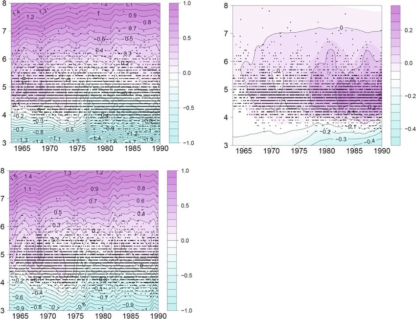
Ogata Progress in Earth and Planetary Science       (2021) 8:8                                                              Page 3 of 20

was first considered for the goodness-of-fit of the surface                  conjugate gradient method and the quasi-Newton linear
for the biases. Here, if necessary, the systematic differ-                   search method that were applied in Ogata and Katsura
                                                  ð1Þ   ð1Þ      ð1Þ   ð1Þ   (1988, 1993) and Ogata et al. (1991, 2003).
ence as an extended function ψ θ ≡ ψ θ ðt i ; xi ; yi ; zi
    ð1Þ                                                                         Thus, the empirical Bayesian model with the smallest
: M i Þ of the time, location, depth, and magnitude could
                                                                             ABIC is regarded as having the best fit with respect to
be considered. Haberman and Craig (1988) considered
                                                                             the hyper-parameters. This ABIC value can be compared
only time-dependent biases of the magnitude differences
                                                                             with the ABIC value of the case in which some hyper-
for applying a traditional test statistic, which is equiva-
                                                                             parameters (weights) are very large for very restricted
lent to assuming a piecewise constant function ψθ = ψ(t)
                                                                             cases, such as w2 = w4 = w5 = 108 in (3), which is equiva-
of time.
                                                                             lent to the case in which no temporal systematic change
  Then, the penalized residual sum of squares was
                                                                             in ψθ occurred, namely, no magnitude shift.
considered
                                                                                For the optimized hyper-parameters (weights), the
    PRSS ðθjwÞ ¼ RSS ðθÞ þ penaltyðθjwÞ;                               ð2Þ   minimized PRSS in (2) provides the solution of the coef-
                                                                             ficients θ^ of the smoothed spline function ψθ, which is
to stabilize the convergence of the unique solution. Here,                   known as the maximum a posteriori (MAP) solution,
the penalty function                                                         namely, the ABIC of which should be compared with
                                                                             that of the time-constant case for significance. The pe-
                                   ∂ ψk 2        ∂ ψk 2
    penaltyðθjwÞ∝∬           A fw1 ð    Þ þ w2 ð      Þ :                    nalized log-likelihood functions have a quadratic form
                                    ∂ x           ∂ t
                         2                2               2                  with respect to the parameter, θ, and so, the posterior
                  ∂2 ψ k           ∂2 ψ k         ∂2 ψ k                     function is proportional to the normal distribution, its
          þw3 ð          Þ þ 2w4 ð        Þ þ w5 ð       Þ g dx dt
                   ∂ x2           ∂ x ∂ t          ∂ t2                      integration is reduced to the determinant of the
  with penalty weights w = (w1, ⋯, w5) works against the                     variance-covariance matrix (details are provided in Mur-
roughness of the function (or smoothness constraint).                        ata (1993), Ogata and Katsura (1988, 1993), and Ogata
The weights of the penalty are optimized by considering                      et al. (1998, 2003)).
the following Bayesian framework: First, consider the
prior probability density function:
                                                                             2.1.2 Magnitude shift issues regarding the JMA hypocenter
                         expf − penaltyðθjwÞg                                catalog
    π ðθjwÞ ¼ R                                 ;                      ð4Þ
                     Θ   expf − penaltyðθjwÞgdθ                              Ogata et al. (1998) applied this method to examine the
                                                                             differences between the magnitudes MJ reported by the
where the adjusting weight vector w is called a hyper-                       JMA and body-wave magnitudes (mb) reported by the
parameter. Then, together with the likelihood function,                      National Earthquake Information Center (NEIC) of the
                                                                           US Geological Survey (USGS) Preliminary Determin-
   LðXjθÞ∝ exp − RSS ðθÞ=2σ 2 ;                      ð5Þ                     ation of Epicenters (PDE) catalog in and around Japan
the posterior function is given by                                           during the period 1963–1989. Here, it is assumed that
                                                                             the global NEIC catalog in this period is homogeneous
    posterior ðθjX; wÞ ¼ LðXjθÞ  π ðθjwÞ;                             ð6Þ   after the installation of the World-Wide Standardized
                                                                             Seismograph Network. The magnitude scale MJ of the
which corresponds to the penalized log likelihood. Here,                     JMA catalog before the mid-1970s is based on the defin-
the optimal selection of adjusted weights w   ^ (called                      ition of Tsuboi (1954), determined by the amplitude of
hyper-parameters in the Bayesian framework) is derived                       the displacement-type seismometer. The optimally esti-
by minimizing the Akaike Bayesian information criterion                      mated function ψθin Fig. 1a for the bias indicates that
(ABIC; Akaike 1980; Parzen et al. 1998, pp. 309–332):                        the JMA magnitudes below MJ 5.5 are substantially
                     Z                                                       underestimated in the period after 1976. This occurred
   ABIC ¼ − 2 max posterior ðθjX; wÞ dθ                                      by mixing the calibrated magnitudes for the velocity-
                         w
                  þ 2 dimðwÞ;                                          ð7Þ   type seismographs that measure smaller earthquakes.
                                                                             This magnitude change (magnitude shift) for earth-
where dim(w) is the number of adjusting hyper-                               quakes caused the appearance of a seismic gap offshore
parameters w for maximization.                                               from Tokai District, in the eastern part of the Nankai
  An efficient optimization calculation for the posterior                    Trough. This gap was reported by Mogi (1986) and
model (2) is given in Murata (1993). In the case of the                      others who were concerned with the expected Tokai
general log likelihood function, instead of the residual                     earthquake.
sum of squares in (1), this procedure requires many                             The epidemic type aftershock sequence (ETAS) model
computational repetitions, including the incomplete                          usually fits well to aftershocks and ordinary seismic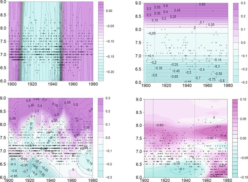
Ogata Progress in Earth and Planetary Science     (2021) 8:8                                                                      Page 4 of 20

 Fig. 1 Smoothed magnitude differences of earthquakes from JMA and USGS PDE catalogs from July 1965–1990 (a, c). The original version of the
 JMA catalog was revised in September 2004. The smoothed magnitude difference of earthquakes in the revised catalog and the original catalog
 is shown in panel b. Panel a compares the magnitude of the original JMA hypocenter catalog and c uses the revised JMA catalog. Contours
 show equidistance of 0.1 difference magnitude unit in the smoothed surface. Higher JMA magnitudes than USGS magnitudes are shown in
 purple. Light blue is used to show the opposite. The vertical red dotted line denotes 1977, when the significant change of the original JMA
 magnitude difference pattern in the range between mb 3.5–5

activities in a self-contained seismogenic region. It sto-               model to the USGS-PDE data with mb ≥ 4.4 and depth≤
chastically decomposes the background seismicity and                     100 km in the same region for the target period of
clustering components. The ETAS model is also useful for                 1963–1995. Furthermore, the significant relative quies-
detecting the period of misfit to the earthquake occur-                  cence in the JMA data for the same target period, depth
rence data. In particular, it is extended to a simple non-               range, and cutoff magnitude as those of the USGS data
stationary ETAS model, meaning that the two-stage ETAS                   was confirmed. These suggested the magnitude shift of
model is applied to estimate a change-point and examine                  the JMA catalog after the mid-1970s, and therefore,
its significance by evaluating whether the two models ap-                whether a magnitude shift occurred in the JMA catalog
plied to the data in the periods before and after the change             after the mid-1970s was explored.
point are statistically significantly different.                            On September 25, 2003, the JMA revised magnitudes
   Ogata et al. (1998) applied the two-stage ETAS model                  based on velocity seismometers so that new velocity
to the JMA earthquake dataset of MJMA ≥ 4.5 for the                      magnitudes must be connected smoothly to the trad-
period 1926–1995 and the central Japan region at 136–                    itional magnitudes based on displacement seismometers
141 °E and 33–37 °N, with a depth of 50 km or shal-                      (see Funasaki 2004). The smoothed differences of JMA
lower, and quiescence relative to the ETAS model was                     magnitudes by the revision are shown in Fig. 1b, which
observed after approximately 1975–1976. In contrast,                     indicates an increase in the new magnitude scale with
there was no relative quiescence by applying the ETAS                    time. Therefore, in the same way, the systematic
Ogata Progress in Earth and Planetary Science (2021) 8:8 Page 5 of 20
magnitude difference of the new JMA hypocenter cata- differences for a bias estimate are different in the range
log against the PDE catalog was reanalyzed. Figure 1c above magnitude Mc = 4.7 of nearly completely detected
shows that a significant bias in time remained, although earthquakes.
the substantial change in the band from M 4.0 to 5.5 To examine which had changed, a third catalog was re-
moved approximately 3 years ahead. quired. Access to any other available catalog for the
Sumatra-Andaman Islands area to investigate the magni-
2.1.3 Magnitude shift issues regarding global hypocenter tude shift was not possible; therefore, Japan and its sur-
catalogs rounding areas were chosen as the study region, with the
Bansal and Ogata (2013) identified seismicity changes assumption that the magnitude shift occurred globally and
approximately 4.5–6 years before the 2004 M 9.1 Suma- was not limited to the Sumatra-Andaman Islands area.
tra earthquake in the Sumatra–Andaman Islands region Here, earthquake magnitudes were provided by the
(90–100 oE, 2–15 °N) using the USGS-NEIC and the USGS-NEIC, ISC, and JMA catalogs. Figure 4a, b shows
International Seismological Centre (ISC) catalogs. These the magnitude differences Mb–MJMA and mb–MJMA of the
authors found that the two-stage ETAS model, with the same earthquakes besides Mb–mb in the Japan area, re-
change point at the middle of the year 2000, provided a spectively, and shows a significantly different mean (bias)
significantly better statistical fit to both datasets of M ≥ of the magnitude difference before and after the same
4.7 than the stationary ETAS model throughout the en- time as the change point time in the Sumatra-Andaman
tire period. However, Fig. 2 shows that the results after Islands region. Figure 3c, d indicates that the smoothed
the change point differed significantly. The former cata- magnitude differences for bias estimations of Mb–MJMA
log implied the activation relative to the predicted ETAS are significantly larger than those of mb–MJMA in the
seismicity after the change point, whereas the latter indi- range above about magnitude Mc = 4.7 of nearly com-
cated the diametrically opposite, namely, the relative pletely detected earthquakes.
quiescence. It was concluded that the magnitude shift was likely to
Magnitude shifts either in the ISC catalog or in the have taken place in the ISC catalog and that Mb was
NEIC catalog after the change point time were, there- underestimated during this time. The lowering of the
fore, suspected. Figure 3a, b shows significantly different ISC magnitudes in the year 1996 was likely due to the
distributions (both mean and variability) of the magni- use of the International Data Centre (IDC) amplitude
tude differences between the NEIC catalog and the ISC data of the Comprehensive Nuclear Test Ban Treaty
catalog before and after the change point time. Figure Organization (CTBTO). In contrast, the NEIC discontin-
3c, d demonstrates that the smoothed magnitude ued the use of the IDC data because the IDC amplitudes
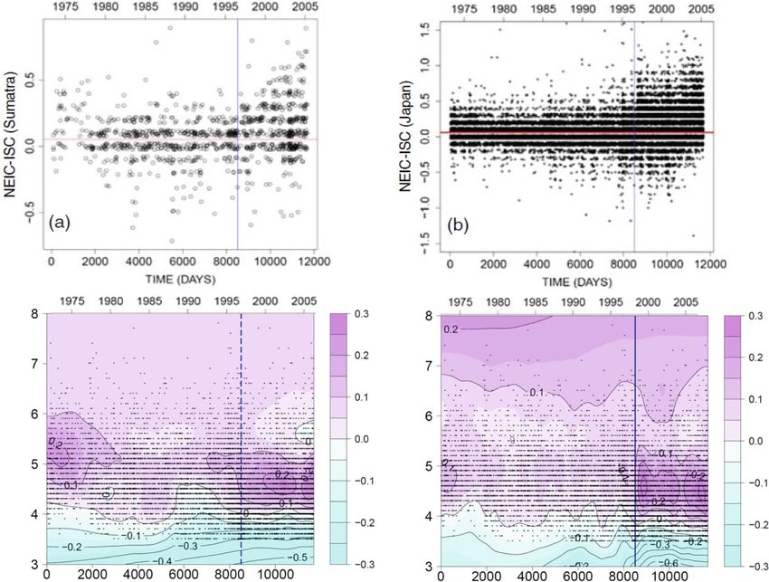
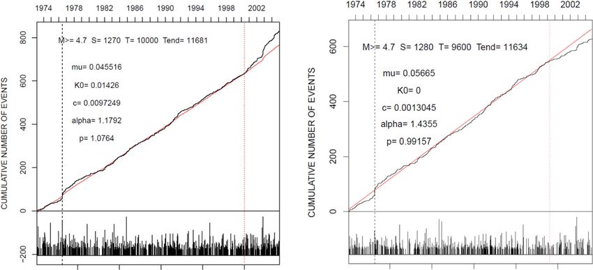
Fig. 2 Opposite seismicity changes between NEIC and ISC catalogs. Estimated cumulative curves of the ETAS model to data from July 1976 until
the M9 Smatra earthquake (December 25, 2004) in the Sumatra-Andaman Island region (see text for the region). The data presented are from the
period up to the maximum likelihood estimate of change-point (red vertical dashed line for July 18, 2000) and the extrapolated ones to the rest
of the period, for the data from a the NEIC PDE catalog and b the ISC catalog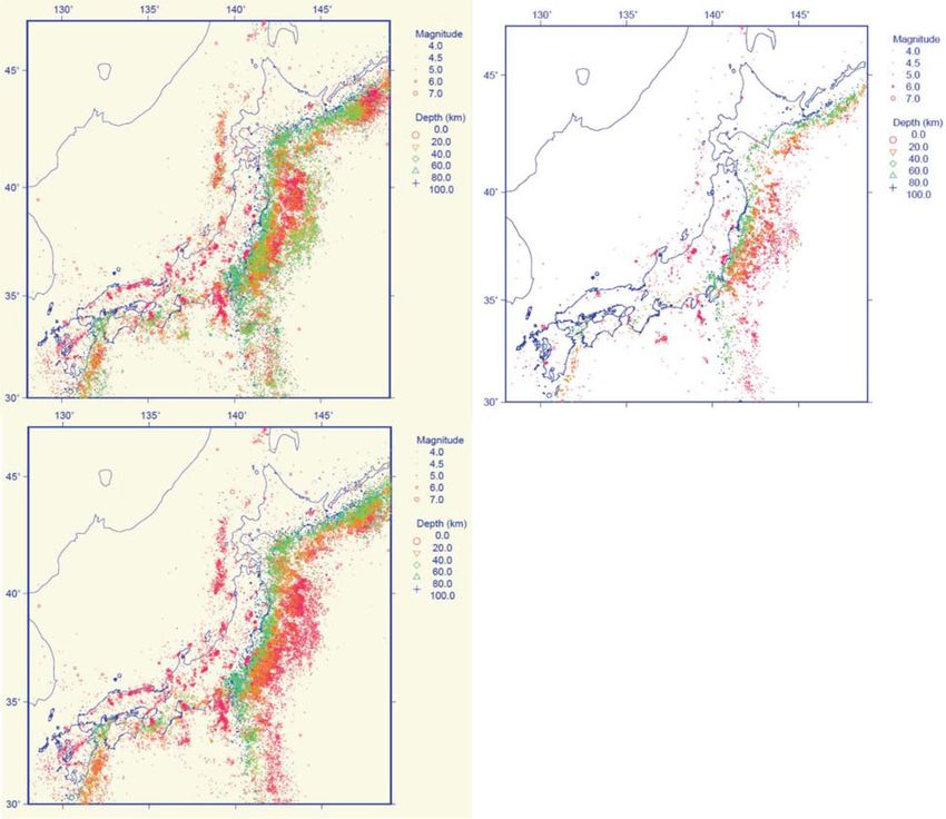
Ogata Progress in Earth and Planetary Science            (2021) 8:8                                                                                 Page 6 of 20

 Fig. 3 Magnitude differences in USGS body wave magnitude mb and ISC body wave magnitude Mb (1973–2005). Mb–mb is shown in the a Sumatra area and
 b Japan area. Because the magnitude differences are 0.1 interval unit, the magnitude differences are plotted with small perturbations. The horizontal red lines
 are mean differences during the earlier period until 8500 days. The smoothed surfaces of Mb–mb on the plane of mb over the period are shown in c Sumatra
 area and d Japan area. Contours show an equidistance of 0.1 magnitude unit differences of the smoothed surface, and thin and thick purple show higher
 magnitudes differences than thin and thick light blue. The horizontal light blue line represents the lowest magnitude of completeness, Mc = 4.7. The vertical
 dark blue lines show changes of the magnitude difference pattern in the range where plots were highly changed

were obtained with a different amplitude measuring pro-                            Poisson process for great earthquakes, which resulted in
cedure than that used at the NEIC, and implied a sys-                              the magnitude heterogeneity of the earlier global catalog
tematic lowering of the magnitude using IDC                                        of the twentieth century of large earthquakes.
amplitudes (Dewey J.W. April 1, 2011, personal commu-                                 Abe (1981) edited a catalog of global earthquakes of
nication). The adoption of the IDC data took place sim-                            magnitude 7 and over for the period 1904–1980. In
ultaneously globally, including both the Sumatra-                                  homogenizing the catalog, the author consistently ad-
Andaman Islands and Japan.                                                         hered to the original definitions of surface-wave mag-
                                                                                   nitude (MS) given by Gutenberg (1945) and
2.1.4 Hypocenter catalog of global shallow large                                   Gutenberg (1956) to determine surface wave magni-
earthquakes in the twentieth century                                               tude MS based on the amplitude and period data
Based on the fractal and self-similar features of earth-                           listed in Gutenberg and Richter’s unpublished notes, bul-
quakes, it is statistically known that the occurrence of                           letins, from stations worldwide, and other sources. Later,
earthquakes is long-range dependent in time as well as                             Abe and Noguchi (1983a, 1983b) added earthquakes that
in space. This applies to large earthquake sequences                               occurred in the early period 1897–1917. Some corrections
worldwide. This section criticizes conventional statistical                        were made by Abe (1984). These catalogs provide a
tests that use the null hypothesis of the stationary                               complete list of large shallow earthquakes for the period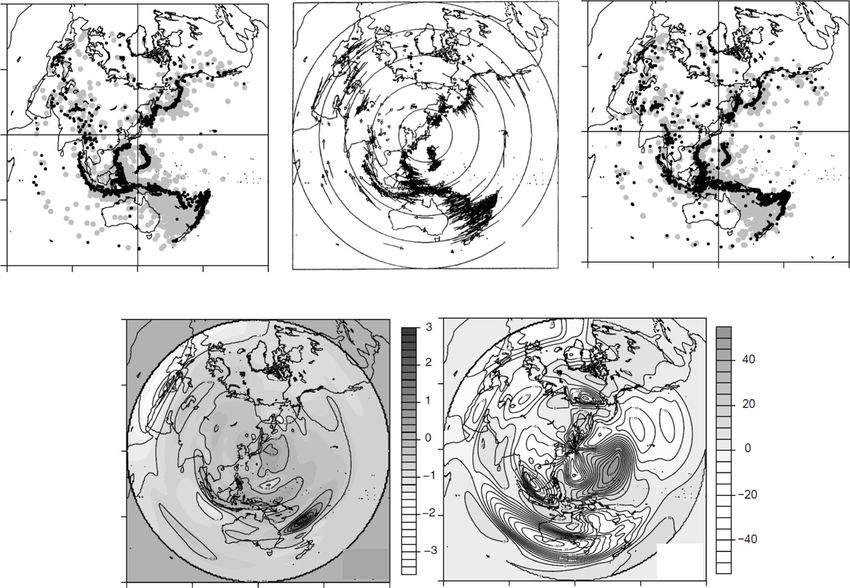
Ogata Progress in Earth and Planetary Science         (2021) 8:8                                                                            Page 7 of 20

 Fig. 4 Magnitude differences of ISC and USGS magnitudes against JMA magnitude MJMA in the Japan area. Magnitude differences a MJMA–Mb, b
 MJMA–mb of the same earthquakes in ISC body wave magnitude Mb and USGS body wave magnitude mb, respectively, relative to the JMA magnitude
 (1973–2005), c smoothed surfaces of Mb–MJMA on the plane of MJMA, d shows the same as c, replacing Mb with mb. Contours show an equidistance of
 0.1 magnitude unit differences of the smoothed surface, and higher magnitudes differences are shown in purple (in contrast to light blue). The vertical
 solid lines in a–d show changes of the magnitude difference pattern in the range where plots were highly changed

1897–1980 (magnitude Ms ≥ 7, depth ≤ 70 km) on a uni-                         However, they did not consider the additions and cor-
form basis. All these catalogs are mutually consistent in                     rections by Abe and Noguchi (1983a, 1983b). The excess
their use of the magnitude scale, hereafter collectively                      before 1908 was almost consistent with the corrections
called “Abe’s catalog.”                                                       of Abe and Noguchi, which was due to the amplitude
  Having examined the broken line-shaped cumulative                           data collected by Gutenberg from the un-dumping
curve of M ≥ 7 earthquakes in Abe (1981) (Fig. 5a),                           Milne seismometers before 1909 being too large due to
Pérez and Scholz (1984) suspected the existence of mag-                       the underestimation of seismometer magnification. In
nitude shifts in Abe’s catalog. This was based on the as-                     consideration of this, the aim of Ogata and Abe (1991)
sumption that the collection of such a large global                           was to determine whether the changes around 1922 and
earthquake should appear as a stationary Poisson                              1948 did not change in seismicity.
process (uniformly random), which corresponds to a                              When hypothesizing that the change in the occurrence
straight linear cumulative curve. These authors conven-                       rate occurred due to magnitude determination bias,
tionally tested Abe’s catalog against the null hypothesis                     Pérez and Scholz (1984) concluded that the MS of the
as a stationary Poisson process (uniformly random) to                         large earthquake in Abe (1981) before 1908, compared
reject the homogeneity of the catalog and then claimed                        to those after 1948, was approximately 0.5 MS unit
that two remarkable changes in the rate around 1922                           overestimated as well as a 0.2 MS unit overestimated in
and 1948 resulted from the inhomogeneity of earthquake                        the period 1908–1948. The smoothed magnitude differ-
catalogs for some instrumental-related reasons.                               ences between the Pérez and Scholz catalog and Abe’s

Ogata Progress in Earth and Planetary Science        (2021) 8:8                                                                          Page 8 of 20

 Fig. 5 Cumulative number of shallow earthquakes. Panels are a with MS ≥ 7 globally, b with MJMA ≥ 6 in the regional area around Japan (1885–
 1980) based on Utsu’s catalog, c with Ms ≥ 7 in low latitude areas, |θ | ≤ 20o, of the world (1897–1980), and d Ms ≥ 7 in high latitude areas, |θ |
 > 20o, of the world (1897–1980), where θ is the latitude

catalog by the estimation method in this study is                            appears non-stationary and non-homogeneous during a
shown in Fig. 6a, whereby, the quasi-periodic vibra-                         one-century period (Fig. 5c, d). This heterogeneity was
tion of the Gibbs phenomena occurred in smoothing                            discussed by Mogi (1974, 1979).
the discontinuous jumps at 1908 and 1948, as ex-                               A twentieth-century catalog of earthquakes in and
pected. It is clear that the argument presented by                           around Japan was edited by Utsu (1982b); this catalog
Pérez and Scholz (1984) strongly depends on their a                          included very many different earthquakes down to ap-
priori assumption of an independent (nonstationary                           proximately M6, much smaller than M7 in Abe’s catalog,
Poisson process) or short-range dependence of earth-                         and the magnitude scale used was independently deter-
quake occurrence. They used the conventional sample                          mined based on the definition of MJMA by Tsuboi
mean difference test (z test), but this should take a                        (1954). The MJMA scale is close to MS, but there is a sys-
higher significance level than the standard hypothesis,                      tematic linear deviation (Utsu 1982b). On average, MJMA
considering the effect of choosing a change point at                         differs from MS by 0.23 units at MJMA = 6.0 and - 0.30
which the difference is most pronounced (Matthews                            units at MJMA = 8.0 (Hayashi and Abe 1984). The mag-
and Reasenberg 1988). Furthermore, the z test is in-                         nitudes of earthquakes for the period 1926–1980 were
appropriate for long-term (inverse power decaying)                           given by the Seismological Bulletins of the JMA, and the
correlated data, such as seismic activity, as discussed                      magnitudes for the period 1885–1925 were determined
below.                                                                       by Utsu (1979, 1982a). Utsu (1982b) compiled these cat-
  If the heterogeneity of the catalog occurs because of                      alogs into one complete catalog with M ≥ 6 for the
instrument error, these two cumulative patterns are ex-                      period 1885–1980. Its catalog for shallow earthquakes
pected to have similar shapes in multiple wide regions.                      (magnitude MJMA ≥ 6, depth 60 km, or shallow depth) in
Figure 5c, d indicates that there were clearly different                     the region 128°–148 °E and 30°–46 °N of Utsu (1982b,
trends in the regions of low latitude bounded by ± 20°                       1985) is hereafter called “Utsu’s catalog.”
and high latitude regions. Furthermore, it is clear that                       It is remarkable that seemingly similar seismic trends
the space-time magnitude pattern of global seismicity                        are observed despite different magnitude determinations
Ogata Progress in Earth and Planetary Science        (2021) 8:8                                                                         Page 9 of 20

 Fig. 6 Smoothed surfaces of magnitude differences of P&S and E&V catalogs against Abe catalog. a MP&S–MABE, b ME&V–MABE on the plane MABE
 against the elapsed time (1897–1980) for global earthquakes, c MABE–MUTSU, and d ME&V–MUTSU on the plane MUTSU over the period in years for Japan
 region. High magnitude differences are shown in purple (in contrast to than light blue). The vertical dotted lines in a–d denote 1922 and 1948

during the same period in Japan (Fig. 5b) and high-lati-                    variation of seismic frequency in high-latitude regions
tude regions of the world (Fig. 5d). It is notable that,                    and in the regional area around Japan, obtained from in-
above a magnitude threshold of completely detected, the                     dependent catalogs, suggests an external effect, such as
number of earthquakes in Japan and neighboring regions                      large-scale motion of the Earth rather than the presup-
comprises approximately 20% of the globe, and also that                     posed heterogeneity of the catalogs.
the Utsu’s catalog (M ≥ 6) includes approximately 10                          The broken line-type cumulative curve for major glo-
times the number of earthquakes in the same area than                       bal earthquakes as appeared in Abe’s catalog (Fig. 5a)
in Abe’s catalog (M ≥ 7). Despite such different magni-                     can be interpreted as follows. This persistent fluctuation
tude thresholds, we see the similarity between Fig. 5b, d                   or trend in appearance being very common in various
whereby, the seismicity rates in Japan and globally high                    geophysical records can be understood in relation to the
latitude areas were high in the 1920s to the 1940s and                      long-range dependence. This is supported by the disper-
gradually decreased until 1980. When assuming the Gu-                       sion-time diagrams, spectrum, and analysis of the R/S
tenberg–Richter law, this similarity in the two independ-                   statistic (Ogata and Abe 1991) for the occurrence times.
ent catalogs suggests that the catalogs reflect the change                  The apparent long-term fluctuation can be reproduced
in the real seismic activity rather than the suspected edi-                 by a set of samples from a stationary self-similar process.
torial heterogeneity of the global catalog. Furthermore,                      The self-similarity or long-range dependence of a time
the smoothed magnitude differences between Utsu’s and                       series can be examined statistically by empirical plots of
Abe’s catalogs (Fig. 6c) ensure that both have no magni-                    earthquake sequences (Hurst 1951; Mandelbrot and
tude shifts over time, which implies the magnitude shift                    Wallis 1969a, 1969b, 1969c; Ogata 1988; Ogata and Kat-
of the Pérez and Scholz catalog due to Fig. 6a, as relative                 sura 1991; Ogata and Abe 1991). According to these au-
to those of Utsu’s catalog in Japan. The synchronous                        thors, a much higher significance level is required for
Ogata Progress in Earth and Planetary Science   (2021) 8:8                                                                  Page 10 of 20

the null hypothesis of stationary long-range dependence       Matsushiro, central Japan. The Seismological Observa-
of the data regardless of declustering, because the major-    tory of the JMA at Matsushiro has an array of stations
ity of decluster algorithms seem to remove short-range        called the Matsushiro Seismic Array System (MSAS),
dependence, and complete removal of dependent shocks          which consists of seven telemetering stations located
other than aftershocks is difficult for such data with        equidistantly on a circle of radius of approximately 5
long-range dependence. Furthermore, the implementa-           km, and at its center. The MSAS locates a focus by a
tion of a z test procedure should be carefully checked in     combination of the azimuth of the wave approach and
seismicity studies.                                           the epicentral distance (i.e., distance to the epicenter
   Nevertheless, this claim of the heterogeneity of Abe’s     from the origin of the array), and thus, the MSAS plays
catalog by Pérez and Scholz (1984) was adopted by Pacheco     various roles not only in reporting the seismic wave ar-
and Sykes (1992), who essentially followed the same magni-    rival times and related data to central institutions in
tude-shift modification for the period 1900–1980 to convert   Japan and the world, but also in quickly detecting and
surface wave magnitudes to moment magnitudes by the           determining locations. This includes those of possible
empirical relation (Ekström and Dziewonski 1988). Inciden-    nuclear experiments as one of the IDC of CTBT.
tally, there is an apparent change-point in 1978 for their      Let an epicenter location estimated by the MSAS be (Δi,
catalog for the period 1969–1990 in Pacheco and Sykes         ϕi) in the polar coordinates centered at the MSAS origin,
(1992) (Fig. 5b), but they made no interpretation for this    and the corresponding true location of beðΔ0i ; ϕ 0i Þ. Here, it is
particular change in the cumulative curve.                    assumed that each earthquake location of the USGS-PDE
   Engdahl and Villaseñor (2002) adopted these moment         catalog is the true location for the period 1984–1988. The
magnitudes and compiled the CENT7.CAT database in             structure of the bias was then analyzed with
the centennial catalog. However, 62% of earthquakes
with Mw ≥ 7 before 1976 were based on the seismic mo-             Δ0i ¼ Δi þ f ðΔi ; ϕ i Þ þ εi ;                                    ð8Þ
ment catalog by Pacheco and Sykes (1992), most of
                                                                  ϕ 0i ¼ ϕ i þ f ðΔi ; ϕ i Þ þ ηi ;                                  ð9Þ
which was based on the conversion of surface wave mag-
nitude MS to seismic moment M0 and then to Mw                 for i = 1 , 2, . . . , N, where εi and ηi are unbiased mutu-
through an empirical formula (see Noguchi (2009) for          ally independent errors owing to the reading errors,
more issues and details). Incidentally, CENT7.CAT led         whereas the functions f and g are the bias functions that
to a seemingly broken line shape in 1948 for the cumu-        are dependent upon the locations determined by the
lative number throughout the twentieth century (e.g.,         MSAS.
see Fig. 4 in Noguchi 2009, M ≧ 7.0)). Figure 6b, d             Whether these error data are useful for estimating the
shows the magnitude differences of the Engdahl and Vil-       standard deviation of the error {ηi} in (9) was then inves-
lasenor catalog relative to Abe’ catalog and Utsu’s cata-     tigated. That is to say, whether ηi ~ N(0, s2 σ 2i ) for some
log, respectively; both of which remain the effect of the     constant s2. In contrast, for the other error εi in (8), it
discontinuous magnitude shift between Abe’s and the           has been empirically determined that the estimation
Pérez and Scholz catalogs in the magnitude range              error of the epicentral distance Δ may be roughly pro-
greater than M6.5. Such earthquake catalogs in the            portional to Δ1/2. Whether this could improve the fit to
twentieth century should, therefore, be used as basic         the data was also investigated.
data to evaluate damaging earthquakes, while carefully          Each spatial function f and g was parameterized by
considering the issues outlined here.                         cubic two-dimensional B-spline functions in the follow-
                                                              ing way: A disc A with radius R of epicentral distance
2.2 Location correction of earthquake catalogs                from the origin in polar coordinates was regarded as a
Similar to replacing magnitudes by location (longitude,       rectangle [0, R] × [0°, 360°) in the ordinary Cartesian co-
latitude, or depth) in the penalized sum of squares dis-      ordinates and was equally divided into MΔ × Mϕ rect-
cussed above, a quasi-real-time correction of the hypo-       angular subregions. For each f and g, the spline
center location can be performed. Revealing systematic        coefficients θ whose number is M = (MΔ + 3) × (Mϕ +
errors in a catalog is a serious subject of seismological     3) was estimated. For the explicit definition of the bi-
research.                                                     cubic B-spline function, see Inoue (1986), Ogata and
                                                              Katsura (1988, 1993), and Ogata and Abe (1991). Then,
2.2.1 Real-time correction of the epicenter location to       the sums of squares of the residuals was considered,
calibrate global earthquake locations                         given by
A similar analysis was applied for the real-time correc-
tion of epicenter locations. For example, Ogata et al.                                X
                                                                                      N
                                                                                                                  2
(1998) utilized this model to calibrate global earthquake         SS distance ðθÞ ¼         fΔ0i − f θ ðΔi ; ϕ i Þg =ðσ 2 Δ2i Þ     ð10Þ
                                                                                      i¼1
location estimates from a small seismic array at
Ogata Progress in Earth and Planetary Science (2021) 8:8 Page 11 of 20
X
N 2 significantly different. Thus, the following model to de-
SSazimuth ðθÞ ¼ ϕ 0i − g θ ðΔi ; ϕ i Þ =σ ðϕ i Þ2 ð11Þ termine the depth bias was considered:
i¼1
z0i ¼ zJMA
i þ h xJMA
i ; yJMA
i ; zJMA
i þ εi ; ð12Þ
where 9801 parameters (i.e., MΔ = Mϕ = 96) were used
for estimations. It was assumed that the functions f and for i = 1, 2, ..., N, where h is the bias function that is
g for the biases were sufficiently smooth for the stable dependent on the locations determined by the JMA net-
estimation of a large number of coefficients. The same work, whereas εi~N(0, σ2) represents unbiased independ-
penalties were considered for functions f and g, as in Eq. ent residuals. Here, the bias function h (x, y, z) is a 3-
1 replacing ψ by f and g, for (10) and (11), and x and t dimensional piece-wise linear function defined on a 3D
by Δ and ϕ, respectively. Then, the optimal minimiza- Delaunay tessellation consisting of tetrahedrons whose
tions of the penalized square sum of residuals by the vertices are the nearest four earthquake hypocenters.
same method as given in the magnitude shift, subsubsec- Namely, each Delaunay tetrahedron provides a flat sur-
tion Statistical models and methods for detecting magni- face (piecewise linear function), where the four heights
tude biases. More details and computational methods of of the flat surface are determined at the tetrahedron ver-
the ABIC procedure with an efficient conjugate gradient tices, and the height of the piecewise flat surface at any
algorithm are described in Ogata et al. (1998). point location is linearly interpolated within the tetrahe-
Real-time correction of the epicenter location utilized dron that includes a JMA hypocenter. The residual sum
this model to calibrate the global earthquake location es- of squares was considered
timates from a small seismic array at the Japan Meteoro-
logical Agency Matsushiro Seismological Observatory, XN 2 2
RSS θ; σ 2 ¼ z0i − hθ xJMA
i ; yJMA
i ; zJMA
i =σ
and this has been adopted for operational determina- i¼1
tions for the Matsushiro catalog. ð13Þ
The USGS epicenters in Fig. 7a are much more accur-
ate than those of the MSAS locations of earthquakes, with a penalty function for the smoothness constraint
where their differences are shown in Fig. 7b. Using the
model and method described above, we had smoothed ∂ hθ 2 ∂ hθ 2
penaltyðθjwÞ ¼ ∭ V w1 þ w2
biases in polar coordinates, as shown in Fig. 7d, e, which ∂x ∂y
can be used for the automatic modification of the future ∂ hθ 2
MSAS coordinates, as shown in Fig. 7c, without knowing þ w3 dx dy dz ð14Þ
∂z
the USGS epicenters. This supports the stability of the
solutions of many parameters, as shown in Fig. 7d, e. Then, the optimal minimizations of the penalized
This result suggests that such systematic biases of square sum of residuals by the same method as given in
MSAS epicenter locations reflect the accurate use of the the subsection “Magnitude shift.”
vertical structure of the P wave velocity model for the Two particular catalogs to compensate for the routine
Earth’s interior (Kobayashi et al. 1993). In addition, we JMA catalog were then utilized in the following exam-
provided discussions with figures of small regional biases ples. First, offshore earthquakes were determined from
of the residuals in Ogata et al. (1998). the observation network in the inland area of the To-
hoku region, and therefore, the depths were determined
2.2.2 Quasi-real-time correction of the depth location of with large deviations in the vertical direction. Umino et
offshore earthquakes al. (1995) determined depths of the epicenters using the
A correction method for the routinely determined hypo- sP wave; that is, the S wave from the epicenter reflected
center coordinates in the far offshore region is given by on the surface of the ground and converted to a P wave
considering the source coordinates of an earthquake that and propagated to the observation point. According to
occurred offshore. Offshore earthquakes are determined this method, the offshore plate boundary earthquake and
only on one side from the observation point in the in- the double seismic surface in the Pacific Plate are accur-
land area, and therefore, the depth is determined with ately determined.
low accuracy and with large deviations. The aim was to Ogata (2009) compared the hypocenters ðx0i ; y0i ; z0i Þ of
compensate for biases that are location-dependent. the Umino catalog and the earthquakes determined this
Let ðxJMA
i ; yJMA
i ; zJMA
i Þ be the hypocenter coordinates of way with those of the JMA catalog ðxJMA
i ; yJMA
i ; zJMA
i Þ and
the earthquake i = 1, 2,…, N, and be ðx0i ; y0i ; z0i Þ the true then estimated the depth deviation in a Bayesian manner
hypocenter coordinates of the corresponding earth- by assuming model (13). The constraint that the devi-
quake. For simplicity, it is assumed that the epicenters ation of the nearest earthquake, which is the vertex of
are very close to each other, but the depths are each tetrahedron by 3D Delaunay division was almostOgata Progress in Earth and Planetary Science (2021) 8:8 Page 12 of 20
Fig. 7 Correction of the epicenter locations determined by the local MSAS array for global earthquakes. Epicenter locations (gray disks) for earthquakes
determined by MSAS; a earthquakes occurring in 1984–1988 and c earthquakes occurring in 1989–1992. The geographical world map is drawn by a polar
coordinate system whose center is the location of the MSAS origin in central Japan. Black disks in a indicate USGS locations and b difference of epicenter
locations of the same earthquake. An arrow indicates the shift from the MSAS location to the USGS location, provided that the differences of epicentral distance
and azimuth are within 2o and 25o, respectively. These are used to minimize by the sum of least squares under a smoothness constraint (see text). The black
disks in c are compensated locations from the MSAS data (gray disks) in c by the estimated bias functions f and g, shown in d and e, respectively. Contour
plots in the panels d and e show the bias functions f for epicentral distance and g for azimuth in Eqs. (10) and (11), respectively, which are estimated using the
data during 1984–1988 in Fig. 7a. The function f varies from − 3.5° to 2.5° in the angular distance, and the contour interval is 0.5°. The function g varies from −
45.0° to 50.0°, and the contour interval is 5.0°. Areas of negative function values are white
the same value as the prior distribution, optimized by system for Earthquakes and Tsunamis (DONET) and the
the ABIC method, and the optimal strength of the con- Seafloor Observation Network for Earthquakes and Tsu-
straint w = (w1, w2, w3) in (14) was determined. namis along the Japan Trench (S-net), will be effectively
Then, the result of the transformation works ^zi ¼ zi used as the target earthquake for depth correction of the
JMA epicenter.
þh^ ðxi ; yi ; zi Þ for any JMA hypocenters that are linearly
θ Second, the F-net Broadband Seismograph Network
interpolated depending on the Delaunay tetrahedron catalog of NIED (2016) is another useful catalog to
that the hypocenter location was included. Figure 8 indi- compensate the JMA catalog. Each earthquake depth
cates how the original JMA hypocenters were modified of the F-net was optimized by waveform fitting, given
in each region. In addition, in the Nankai Trough area, the fixed epicenter coordinate. Although the accuracy
hypocenter correction is also desired to compare the of the depths of F-net is given in a 3-km unit, this is
past JMA catalog from the viewpoint of the forecast still useful for removing the offshore biases of the
strategy of the expected large earthquake. It is hoped JMA depths. Figure 9 indicates how the original JMA
that the epicenter data accumulated by ocean bottom hypocenters are modified in, and around, the main-
seismometers, such as the Dense Ocean floor Network land Japan region.Ogata Progress in Earth and Planetary Science (2021) 8:8 Page 13 of 20
Fig. 8 Depth corrections of offshore earthquakes from the JMA catalog (example 1). a Routinely determined M ≥ 3 earthquake hypocenters in
JMA catalog during 2000–2006 and b corrected hypocenters using the sP waves by Umino et al. (1995) for the same earthquakes (left panels)
2.3 Detection rates of earthquakes and b values of the magnitudes at which earthquakes are partially de-
magnitude frequency tected (Ringdal 1975), so that μ + 2σ provides the
Most catalogs covering a long time period are not magnitude at which 97.5% of earthquakes are de-
homogeneous because the detection rate of smaller tected. Then, a model of magnitude frequency distri-
earthquakes changes in time and space due to the devel- bution for observed earthquakes
opment of seismic networks changing over a long period
of time. In contrast, many aftershocks occur immediately
λðMjb; μ; σ Þ ¼ 10a − bM qðMjμ; σ Þ
after a large earthquake, with waveforms that overlap on Z
the seismometer records, making it difficult to effectively 10a − bM M − ðx − μÞ2 =2σ 2
¼ pffiffiffiffiffiffi e dx; ð15Þ
determine the hypocenters and magnitudes of smaller 2π σ − ∞
aftershocks immediately following earthquakes. There-
fore, many aftershocks immediately after a large earth- was considered, to examine space-time inhomogeneity
quake are not detected or located. by assuming that the parameters (b, μ, σ) are not con-
The aim was to separate real seismicity from the stants but represented by functions of time t and/or lo-
catalog heterogeneity. One method for doing so is a cation (x, y). Then, given a data set of times, epicenters,
traditional method that restricts earthquakes above a and magnitudes (ti, xi, yi, Mi), log-likelihood was consid-
completely detected magnitude, but this loses a large ered (Ogata and Katsura 2006), given in the form
amount of data. A frequency distribution was used
for all detected earthquakes by assuming the Guten- Z
X
N ∞
berg–Richter law for magnitude frequency and model- ln Lðb; μ; σ Þ ¼ ln λðt i ; Mi jb; μ; σ Þ − ∬ A λðt; Mjb; μ; σ Þ dMdt
ing detection rate of earthquakes of magnitude such i¼1 −∞
that 0 ≤ q(M| μ, σ) ≤ 1, which is a cumulative function ð16Þ
of the normal distribution where the parameter μ rep-
resents the magnitude value at which 50% of earth-
for time evolution or
quakes are detected and σ relates to a range ofOgata Progress in Earth and Planetary Science (2021) 8:8 Page 14 of 20
Fig. 9 Depth corrections of offshore earthquakes from the JMA catalog (example 2). a Routinely determined M ≥ 3 earthquake hypocenters in JMA catalog
(2000–2006) and c corrected hypocenters using of F-net catalog (b)
2.3.1 Modeling detection rate changes over time
X
N The south coast of Urakawa (Urakawa-Oki, Fig. 10a) is lo-
ln Lðb; μ; σ Þ ¼ ln λðxi ; yi ; M i jb; μ; σ Þ cated approximately 142.5 °E, 42 °N in Hokkaido, Japan,
i¼1Z ∞
and has been an active swarm-like earthquake zone for a
− ∬A λðx; y; Mjb; μ; σ Þ dMdxdy long period of time. The observed swarm activity from
−∞
1926 to September 1990, with a depth of h ≤ 100 km, was
ð17Þ
examined, and the data were chosen from the JMA Hypo-
center Catalog. Figure 10b includes the cumulative curve
for spatial variation, in place of the sum of squares and magnitudes versus occurrence times of all earth-
in the above, with penalties against the roughness of quakes with determined magnitudes. The apparently in-
b ‐ , μ‐ and functions σ‐ of time t and/or location (x, creasing rate of events (i.e., increasing slope of cumulative
y). The optimal strengths of the roughness penalties, number curve in Fig. 10b) does not always mean an in-
or smoothing constraints, are obtained, and the solu- crease in seismic activity. From the magnitude versus time
tions are useful for analyzing b value changes and plot (Fig. 10b), it was observed that the number of smaller
seismicity. earthquakes increased with time, indicating an increase inOgata Progress in Earth and Planetary Science (2021) 8:8 Page 15 of 20 Fig. 10 Temporal detection rate analysis of earthquakes. Detected earthquakes off the coast of southern Urakawa (Urakawa-Oki, (A)), Hokkaido (1926–1990), B cumulative number of earthquakes by year since 1926 with the corresponding magnitude versus occurrence time plot, Ca b values (b = β loge 10) against time in years, Cb μ values (50% detection rate) against time in years, Cc σ value against time in years, and D magnitude frequency histograms (“+” sign) of in time spans Da 1926–1945, Db 1946–1965, Dc 1966–1975, Dd 1976–1983, and De 1984–1990 with the estimated frequency-density curves at the middle time (indicated by the squared a–e in panel C) in the corresponding time spans, where x-axis is for magnitude and y-axis is the frequencies given in logarithmic scale. Theoretically calculated two-fold standard error curves are provided for each interval the detection capability of earthquakes in the area. In con- (described in the Appendix of Ogata and Katsura trast, the steepest rise of the cumulative curve in March (1993)). Further subdivisions did not provide any signifi- 1982 includes the aftershock activity of the 1982 M 7.1 cant improvement in the ABIC value, and hence, the Urakawa-Oki earthquake. number of B-spline coefficients of the three functions, To conventionally obtain the b value change of the real b, μ, and σ of time t is 3 × (20 + 3). seismic activity by removing the effect of detection cap- Firstly, the ABIC values for the goodness-of-fit of the ability, it is necessary to use data from earthquakes whose penalized log likelihood (Good and Gaskins 1971) were magnitudes exceeded the cutoff magnitude above which compared between the same weight values and inde- almost earthquakes were detected throughout the ob- pendently adjusted distinctive weights penalties posed to served time span and region. The cutoff magnitude for the the b-, μ-, and σ-functions for the strength of the complete earthquake detection in this area since 1926 is smoothness constraint. In this case, the latter approach MJ 5.0. This leads to significant data waste (cf., Fig. was better, and thus, the estimated function in Fig. 10B(a)) so instead, all the data of detected earthquakes for 10C(a) shows that the trend of b value change appears an unlimited range of magnitudes were included. In total, to decrease linearly in the range of 65 years. Figure 1249 events were considered for this example. 10C(b) shows that the magnitude of 50% detected earth- The entire time interval was divided into 20 subinter- quakes decreased from MJ 5.0 to MJ 3.0 by 1990. Figure vals of equal lengths for the knots of the cubic B-spline 10C(c) shows the range of the partially detected
Ogata Progress in Earth and Planetary Science        (2021) 8:8                                                                       Page 16 of 20

magnitude, which tends to be large when the seismic ac-                     2.3.2 Spatial detection rate changes immediately following
tivity is low.                                                              a large earthquake
   To determine the significance of the patterns of the b,                  Omi et al. (2013) demonstrated the retrospective fore-
μ, and σ values, their variability distributions of the esti-               casting aftershock probability in time within 24 h by
mates were computed by the Hessian matrix of posterior                      using the USGS-PDE catalog aftershock activity immedi-
distribution (6) around the MAP solution, where the                         ately after the 2011 Tohoku-Oki Earthquake of M 9.0 in
likelihood function is replaced by the one in (16). The                     Japan. Although the JMA provides many more after-
two-fold standard error curves are shown in Fig.                            shocks, spatial heterogeneity is conspicuous, and the
10C(a)–(c), which indicates that the standard error is                      time evolution of aftershock detection becomes complex.
small when the event occurrences are densely observed.                      Here, the focus was on the spatial detection rate within
   To confirm the goodness-of-fit of the estimated model,                   one day after the M 9.0 event.
the entire time interval from 1926 to the end of Septem-                       The green and red dots in all panels in Fig. 11 indicate
ber 1990 was divided into five subintervals at the end of                   the epicenter locations of all detected earthquakes by the
1945, 1965, 1975, and 1983. Then, the histogram of the                      JMA network in mainland Japan, and its vicinity with a
magnitude frequency for each subinterval was compared                       depth up to 65 km after the M 9.0 earthquake until the
with the estimated frequency function of magnitude in                       end of the day. Earthquakes are highly clustered in
(15) at the middle time point t (squared a–e) of the cor-                   space, and therefore, the Delaunay-based functions ra-
responding subinterval in Fig. 10C(a)–(c). Figure                           ther than cubic spline functions were adopted.
10D(a)–(e) demonstrates such a comparison, where the                           A 2D Delaunay tessellation, based on these and add-
error bands for the estimated curve are of the first-order                  itional locations on the rectangular boundary, including
approximation around the marginal posterior mode (de-                       the corners, was developed. Then, the Delaunay-based
tails are provided in Ogata and Katsura (1993). A good                      functions for the location-dependent parameters were
coincident between the histogram and estimated curves                       defined. The coefficients are values at the epicenters,
is transparent from Fig. 10D(a)–(e).                                        and the parameter value at any location is linearly

 Fig. 11 Examples of spatial detection rate analysis of aftershocks. Estimated surfaces for earthquakes shallower than 65 km detected by the JMA
 network 1 day after the 2011 M9 Tohoku-Oki earthquake. Earthquakes are shown as green and red dots. a b values with contour interval 0.05, b μ
 value (magnitude with 50% detection rate) with contour interval 0.05, c σ value with contour interval 0.01, and d–f 97.5% detection rate of M 2.0,
 M 3.0, and M 4.0 earthquakes, respectively, with contour interval 0.1 (10%)
Ogata Progress in Earth and Planetary Science (2021) 8:8 Page 17 of 20
interpolated. Here, the piecewise linear functions fk(x,y), Figure 11d–f shows the interpolated images of the op-
k = 1,2,3, are defined in the following forms: b(x,y) = timal MAP estimates (solutions) of the parameter func-
exp{f1(x,y)}, μ(x,y) = exp{f2(x,y)}, and σ(x,y) = exp{f3(x,y)}, tions and spatial distribution of 97.5% detected
to avoid negative values, where each triangle provides a earthquakes of the M 2.0, M 3.0, and M 4.0 earthquakes,
flat surface for which the height of the surface at the respectively. The value at each pixel of the graph is cal-
three vertices. At any other point on the surface of the culated as the linear interpolation of the three coeffi-
triangle, the height of the surface can be determined cients of the nearest Delaunay triangle. The detailed
using linear interpolation. images can be shown by magnifying the region where
The log likelihood function (17) of the coefficients of the earthquakes are densely distributed or highly clus-
the parameter functions is considered, and considers the tered, as demonstrated in Ogata and Katsura (1988) (Fig.
penalty function of the form 5). This is an advantage of the Delaunay-based function.
Finally, the Global Centroid Moment Tensor (CMT)
X
K 2 catalog was considered (https://www.globalcmt.org/
∂fk
penaltyðθjwÞ ¼ wk ∬ A CMTsearch.html). The earthquakes are highly clustered
∂x
k¼1
2
along the trench curves in space, and so Delaunay-based
∂fk parameterization, as before, was adopted, rather than
þ dxdy; ð18Þ
∂y cubic spline and kernel functions. First, the b values
using all earthquakes of M ≥ 5.4 for the period 1976–
for the smoothness constraints with K = 3, where the 2006 were estimated, above which the earthquakes of
weights w = (w1, w2, w3) are adjusted as explained for the entire period throughout world are completely de-
(4)–(7), where the penalty and likelihood function is re- tected. The likelihood function for the b value was used
placed by (18) and the one in (17), respectively. In gen- by Aki (1965). Alternatively, this is equivalent to the lim-
eral, the variability is small where the epicenters are ited case of (15), where for q(M| b, μ, σ) = 1 M ≥ 5.4, and
densely distributed, and large where they are sparse, in = 0 otherwise; subsequently, consider the log likelihood
particular, about the boundary of the considered region. (17), which is dependent only on the b function. Thus,
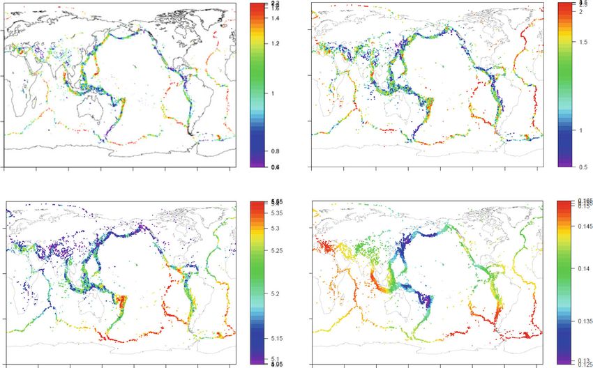
Fig. 12 Optimal MAP solutions for Global CMT catalog. a Estimated b values by using all completely detected M ≥ 5.4 earthquakes and b–d estimated b, μ,
and σ values by using all detected M ≥ 0 earthquakes, respectively. Rainbow colors represent ordered estimates in respective quantities, and the estimated
values are shown by the corresponding color tablesYou can also read