WMO GREENHOUSE GAS BULLETIN
←
→
Page content transcription
If your browser does not render page correctly, please read the page content below
WEATHER CLIMATE WATER

                 WMO GREENHOUSE GAS
                 BULLETIN                                         The State of Greenhouse Gases in the Atmosphere Based on Global
                                                                  Observations through 2020

                 No. 17 | 25 October 2021
ISSN 2078-0796

                   Roughly half of the carbon dioxide (CO2) emitted by              uptake by land ecosystems. Ocean uptake might also be
                   human activities today remains in the atmosphere. The            reduced as a result of higher sea-surface temperatures,
                   rest is absorbed by oceans and land ecosystems. The              decreased pH due to CO2 uptake [3] and the slowing
                   fraction of emissions remaining in the atmosphere,               of the meridional ocean circulation due to increased
                   called airborne fraction (AF), is an important indicator         melting of sea ice [4]. Timely and accurate information
                   of the balance between sources and sinks. AF varies              on changes in AF is critical to detecting future changes
                   a lot from year to year, and over the past 60 years              in the source/sink balance.
                   the relatively uncertain annual averages have varied
                   between 0.2 (20%) and 0.8 (80%). However, statistical            Luckily, information is available from observations
                   analysis shows that there is no significant trend in the         of atmospheric CO2 made at key locations around
                   average AF value of 0.42 over the long term (about               the world from the WMO Global Atmosphere Watch
                   60 years) (see Figure 1). This means that only 42%               (GAW) Programme and its contributing networks.
                   of human CO2 emissions remain in the atmosphere.                 These long-term and accurate observations give direct
                   Land and ocean CO2 sinks have continued to increase              insight into the trend in atmospheric levels of CO2 and
                   proportionally with the increasing emissions. It is              other greenhouse gases (GHGs), as illustrated in this
                   uncertain how AF will change in the future because               and previous editions of the Bulletin. These data can
                   the uptake processes are sensitive to climate and                be combined with other observations (for example
                   land-use changes.                                                of stable isotope ratios and the oxygen/nitrogen
                                                                                    (O2/N2) ratio) and inverse models (that apply atmospheric
                   Changes in AF will have strong implications for                  tracer transport models) and help derive quantitative
                   reaching the goal of the Paris Agreement, namely                 information on the strength of major CO 2 uptake
                   to limit global warming to well below 2° C, and will             processes in the global carbon cycle and analyse AF
                   require adjustments in the timing and/or size of the             and the factors contributing to its changes [5].
                   emission reduction commitments. Ongoing climate
                   change and related feedbacks, such as more frequent              Based on this direct observational information, better
                   droughts and the connected increased occurrence                  projections of CO2 levels for the expected emission
                   and intensification of wildfires [2], might reduce CO2           scenarios can be provided, allowing for improved

                    Figure 1. Fitted estimate of the linear trend in AF (TA) over the period 1960–2016 [1]. Individual estimates of annual mean AF
                    are depicted by the dashed lines using two methods with zero (AF(1)) and a non-zero (AF(2)) carbon budget imbalance. The
                    slightly upward slope of the trend over the period is found to be not statistically significant.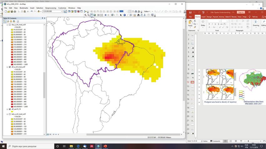
climate projections. Figure 2 shows an example of                                                The recent 2021 GCOS status report [6] recognizes the
an analysis where long-term observations at a single                                             recent improvements in availability of observations
station can be used to determine the distribution of                                             in for example the GAW GHG network and satellite
fossil fuel CO2 emissions between terrestrial and                                                observations, but also points to four main areas that
oceanic sinks, based on the fact that for respiration                                            still need improvements:
and photosynthesis CO2 and O2 co-vary, whereas for
                                                                                                 • Ensuring the sustainability of observations,
ocean gas exchange they do not. Note that the analysis
                                                                                                 • Addressing gaps in the system,
covers a different period than that for Figure 1 and that                                        • Ensuring permanent, free and unrestricted access to the
it does not include all sources of uncertainty, such                                               observations,
as representativeness of the station and calibration                                             • Increasing support for policies driven by the UNFCCC
uncertainties.                                                                                     Paris Agreement.

In order to better support GHG management policies                                               The lat ter point would require more regional
through analysis of natural sinks and fossil fuel                                                observations (in urban and contributing networks
emissions, and to narrow them down to the regional                                               like Integrated Carbon Observation System) over the
or the local level, improved sustainability of the current                                       whole globe. WMO GAW contributes to this for example
in situ network and additional in situ data are needed.                                          through the IG3IS initiative (https://ig3is.wmo.int/, see
This goes hand in hand with increasing remote sensing                                            also GHG Bulletin 12) where an international standard
capacities, especially in currently undersampled                                                 for urban GHG monitoring is being developed.
regions, such as Africa and other tropical regions.

                                       -50

                                                                                       F
                                       -75      2005
Deviation of O2 mole fraction [ppm]

                                      -100
                                                         Ob

                                                                                                                            αF • F
                                                             se

                                      -125
                                                               rva
                                                                  tio
                                                                    ns

                                                                                            2020
                                      -150                                         Z
                                                                                                                           LUC

                                                                            αB • B                                                   αLUC • LUC
                                      -175

                                                                 ΔCa/Δt                            B                   O

                                      -200
                                                             4.7 ± 0.03 Gt C y-1           2.9 ± 0.68 Gt C y-1 3.1 ± 0.65 Gt C y-1

                                                                (44 ± 0.3 %)                  (27 ± 6.3 %)        (29 ± 6.0 %)

                                      -225
                                          360          380              400                    420                440                460          480
                                                                    CO2 mole fraction [ppm]
Figure 2. Analysis of the global carbon budget based on observations of CO2 and O2 at WMO GAW global station
Jungfraujoch, Switzerland [7]. The top-right insert shows the underlying hourly time series for CO2 and the O2 /N2 ratio
from 2005 to 2021. The outcome of the analysis shows that over the 16-year period the percentage of emissions remaining
in the atmosphere is 44% (ΔCa/Δt = 0.44), global biosphere uptake (B) is 27% and global ocean uptake (O) is 29%. The red
line depicts the theoretical changes in CO2 and O2 levels in response to fossil fuel emissions (F) and emission associated
with land-use change (LUC). (Z) shows changes in O2 level due to ocean thermal outgassing.

                                                                                             2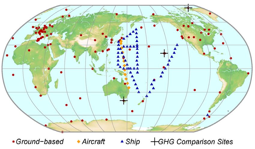
Executive summary
The latest analysis of observations from the WMO GAW in situ
observational network shows that globally averaged surface
mole fractions(1) for CO2, methane (CH4) and nitrous oxide (N2O)
reached new highs in 2020, with CO2 at 413.2 ± 0.2 ppm(2), CH4 at
1889 ± 2 ppb(3) and N2O at 333.2 ± 0.1 ppb. These values constitute,
respectively, 149%, 262% and 123% of pre-industrial (before
1750) levels. The increase in CO2 from 2019 to 2020 was slightly
lower than that observed from 2018 to 2019, but higher than the
average annual growth rate over the last decade. This is despite
the approximately 5.6% drop in fossil fuel CO2 emissions in 2020
due to restrictions related to the coronavirus disease (COVID-19)
pandemic. For CH4, the increase from 2019 to 2020 was higher
than that observed from 2018 to 2019 and also higher than the
                                                                                                        Figure 4. The GAW global network for CO2 in the last decade.
average annual growth rate over the last decade. For N2O, the                                           The network for CH4 is similar.
increase from 2019 to 2020 was higher than that observed from
2018 to 2019 and also higher than the average annual growth rate                                       The WMO GAW Programme coordinates systematic
over the past 10 years. The National Oceanic and Atmospheric                                           observations and analyses of GHGs and other trace species.
Administration (NOAA) Annual Greenhouse Gas Index (AGGI)                                               Sites where GHGs have been measured in the last decade
[8] shows that from 1990 to 2020, radiative forcing by long-                                           are shown in Figure 4. Measurement data are reported by
lived greenhouse gases (LLGHGs) increased by 47%, with CO2                                             participating countries and archived and distributed by the
accounting for about 80% of this increase.                                                             WMO World Data Centre for Greenhouse Gases (WDCGG) at
                                                                                                       the Japan Meteorological Agency.
Overview of observations from the GAW in situ
observational network for 2020                                                                         The results reported here by WDCGG for the global average
                                                                                                       and growth rate are slightly different from the results reported
This seventeenth annual WMO Greenhouse Gas Bulletin                                                    by NOAA for the same years [10], owing to differences in
reports atmospheric abundances and rates of change of the                                              the stations used and the averaging procedure, as well as
most important LLGHGs – CO2, CH4 and N2O – and provides                                                a slight difference in the time period for which the numbers
a summary of the contributions of other GHGs. Those                                                    are representative. WDCGG follows the procedure described
three, together with dichlorodifluoromethane (CFC-12) and                                              in detail in GAW Report No. 184 [11]. The results reported
trichlorofluoromethane (CFC-11), account for approximately                                             here for CO2 differ slightly from previous Greenhouse Gas
96%(4) [8] of radiative forcing due to LLGHGs (Figure 3).                                              Bulletins (by approximately 0.2 ppm) because data are now
                                                                                                       reported on the new CO2 calibration scale WMO CO2 X2019
All percentage contributions to radiative forcing in this Bulletin                                     [12]. Historical data have been converted to the new scale to
are calculated following the methodology in [8], use 1750 as                                           ensure consistency in reported trends.
a reference period and only include LLGHGs.
                                                                                                       The table provides the globally averaged atmospheric
                                                                                                       abundances of the three major GHGs in 2020 and the changes
                               HFCs*
                               HCFCs
                               CFCs*
                               N2O
                                                                                                        Table. Global annual surface mean abundances (2020) and
                                                              Annual Greenhouse Gas Index (AGGI)

                               CH4
                               CO2
                                                                                                        trends of key GHGs from the GAW in situ observational
    Relative Forcing (W.m–2)

                                                                                                        network. Units are dry-air mole fractions, and uncertainties
                                                                                                        are 68% confidence limits. The averaging method is described
                                                                                                        in GAW Report No. 184 [11].

                                                                                                                                       CO2        CH4        N2O

                                                                                                        2020 global mean            413.2±0.2    1889±2    333.2±0.1
                                                                                                        abundance                     ppm         ppb        ppb

                                                                                                        2020 abundance relative
  Figure 3. Atmospheric radiative forcing, relative to 1750,                                                                          149%       262%        123%
                                                                                                        to 1750 a
  by LLGHGs corresponding to the 2020 update of the NOAA
  AGGI [8]. Note that the updated calculation from the 2021                                             2019–2020 absolute
  Intergovernmental Panel on Climate Change (IPCC) Working                                                                           2.5 ppm     11 ppb     1.2 ppb
                                                                                                        increase
  Group I report [9] has not been included in this estimate. The
  “CFCs*” grouping includes other long-lived gases that are not                                         2019–2020 relative
  chlorofluorocarbons (CFCs) (e.g. CCl4, CH3CCl3 and halons),                                                                         0.61%      0.59%      0.36%
                                                                                                        increase
  but the CFCs accounted for the majority (95% in 2020) of this
  radiative forcing. The “HCFCs” grouping includes the three                                            Mean annual absolute
                                                                                                                                       2.40       8.0       0.99
                                                                                                        increase over the last
  most abundant hydrochlorofluorocarbons (HCFCs) (HCFC-22,                                                                           ppm yr–1   ppb yr–1   ppb yr–1
                                                                                                        10 years
  HCFC-141b and HCFC-142b). The “HFCs*” grouping includes
  the most abundant hydrofluorocarbons (HFCs) (HFC-134a,                                                a   Assuming a pre-industrial mole fraction of 278 ppm for
  HFC-23, HFC-125, HFC-143a, HFC-32, HFC-152a, HFC-227ea and                                                CO2, 722 ppb for CH4 and 270 ppb for N2O. The number
  HFC-365mfc) and sulfur hexafluoride (SF6) for completeness,
                                                                                                            of stations used for the analyses was 139 for CO2, 138
  although SF6 only accounted for a small fraction of the radiative
  forcing from this group in 2020 (13%).
                                                                                                            for CH4 and 105 for N2O.

                                                                                                   3                                            (Continued on page 6)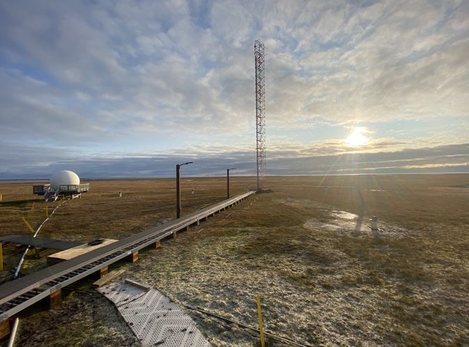
CarbonWatchNZ: using long-term atmospheric CO2 measurements to shed
light on New Zealand’s forest carbon uptake

In New Zealand, forests offset 30% of GHG
emissions, but estimates of forest carbon
uptake remain highly uncertain. The national
inventory report (NIR), which tracks progress
against emissions targets under the United
Nations Framework Convention on Climate
Change (UNFCCC), uses measurements of tree
diameter and height at a national network of
sites to estimate forest carbon uptake [25]. This
approach follows international best practices
guidelines [26], but it may not capture all forest
ecosystem processes adequately.

Independent estimates from atmospheric
CO2 measurements and modelling suggest
that forest carbon uptake may be significantly
underestimated by both the NIR and terrestrial
biosphere modelling [27]. The most recent results
confirm this sink with additional measurements
and modelling and show that it has lasted for at
least a decade (Figure 10).

This additional carbon uptake occurs in one
of the most unlikely places: the south-west of
South Island, a region dominated by mature Figure 11. Average uptake of New Zealand’s terrestrial biosphere
indigenous forests (Figure 11). Indigenous forests between 2011 and 2020 estimated from atmospheric measurements
in New Zealand have long been thought to absorb and modelling.
less carbon than plantation forestry, which is
primarily fast-growing exotic trees. These results
could open a new, more sustainable pathway to planting native forests for carbon sequestration.
manage the country’s forests for carbon uptake However, little is known about the sensitivity
with many environmental co-benefits [27].          of New Zealand’s unique indigenous forests to
                                                   future climate change. Ongoing measurements
New Zealand’s Climate Change Commission will help to understand the sensitivity of these
recently recommended that the country transition forests to climate change and how their carbon
away from relying on plantation forestry towards uptake will respond to a changing world.

Figure 10. Annual average carbon flux from New Zealand’s terrestrial biosphere estimated from the Biome-BGC model (grey) and
from atmospheric CO2 measurements and modelling (green) [27].

                                                             4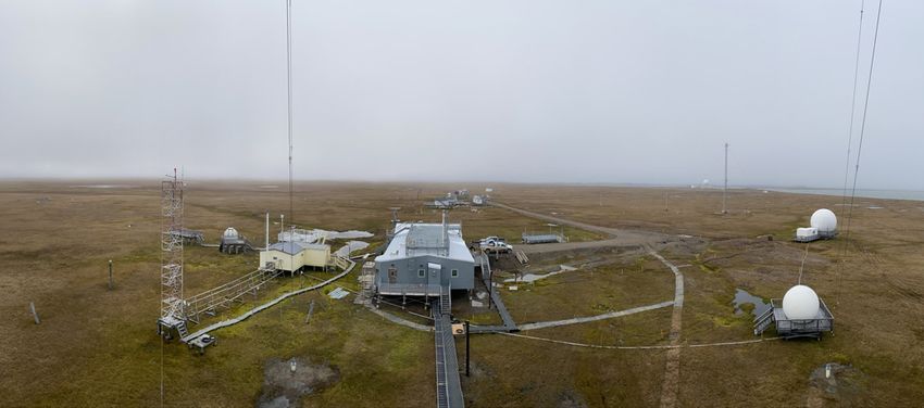
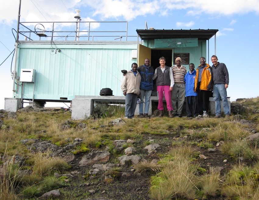
Observations clarify the carbon cycle of tropical regions: Amazonia as
a net CO2 source

              4 000                                                                                                         2

                                                                                       Climatological Flux (gC m-2 day-1)
              3 500

              3 000                                                                                                         1
Height (m)

              2 500

              2 000
                                                                                                                            0
              1500

              1000
                                                                                                                            −1
               500

                    0
                     -4.0 -3.0 -2.0 -1.0 0.0 1.0 2.0 3.0 4.0 5.0                                                            −2
                                    CO 2 - BKG (ppm)                                                                         Jan   Feb Mar Apr May Jun   Jul   Aug Sep Oct Nov Dec

Figure 12. Annual mean vertical profiles at ALF aircraft measurement                   Figure 14. Average monthly means of ALF carbon fluxes during
site in Brazil [28].                                                                   2010–2018. The grey band denotes the standard deviation of the
                                                                                       monthly means, and the solid line show 9-year mean climatological
                                                                                       carbon flux at south-eastern Amazonia [28].
Tropical regions such as Amazonia play an
important role in the global carbon balance.                                           data gathered capture the surface flux balance
Amazonia hosts the Earth’s largest tropical forest,                                    from a large fraction of Amazonia (about 80% of
but as with other tropical regions it has only a few                                   South American Amazon). Overall, 600 CO2 and
of the in situ observations needed to determine the                                    CO aircraft vertical profiles have been collected
large-scale carbon fluxes. To improve estimates                                        between 2010 and 2018 [28].
of Amazonia’s contribution to the global carbon
budget, an aircraft measurement programme                                              Annual mean vertical profiles are shown in
was started in 2010 over four different sites in                                       Figure 12. The south-east region, captured by
this region: Alta Floresta (ALF), Rio Branco (RBA),                                    the ALF site (8.80°S, 56.75°W; see Figure 13), has
Santarém (SAN) and Tabatinga/Tefé (TAB/TEF).                                           the largest CO2 emissions to the atmosphere
The vertical profiles extend from near the surface                                     (Figure 14), followed by the north-east region.
to approximately 4.5 km above sea level and the                                        In contrast, the western sites’ vertical gradients
                                                                                       (not shown here) indicate near-neutral carbon
                                                                                       balance or carbon sinks. The CO2 gradients
                                                                            10˚

                                                                                       from the annual mean vertical profiles and the
                                                                                       estimated carbon fluxes for these sites indicate
                                                                                       that areas that are more affected by land-use
                                                                                       and land-cover change show higher carbon
                                                                            0˚

                                                                                       emissions to the atmosphere. The regions in the
                                                                                       eastern Amazon have very strong dry-season
                                                                                       temperature increases, precipitation decreases
                                                                            -10˚

                                                                                       and large historical deforestation during the last
                                                                                       40 years, while the western regions experience
                                                                                       relatively low levels of human disturbance and
                                                                                       dry-season climate trends.
                                                                            -20˚
                                                                            -30˚

             -80˚         -70˚        -60˚        -50˚        -40˚   -30˚
Figure 13. Footprint of the ALF aircraft measurement site (averaged
area between 2010 and 2018).

                                                                                   5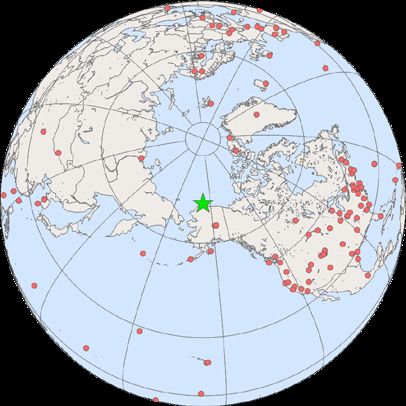
in their abundances since 2019 and 1750. Data from mobile
stations (blue triangles and orange diamonds in Figure 4),
with the exception of data provided by NOAA sampling in the
eastern Pacific, are not used for this global analysis.

The three GHGs, see the table, are closely linked to anthropogenic
activities and interact strongly with the biosphere and the
oceans. Predicting the evolution of the atmospheric content
of GHGs requires a quantitative understanding of their many
sources, sinks and chemical transformations in the atmosphere.
Observations from GAW provide invaluable constraints on
the budgets of these and other LLGHGs, and they are used to
improve emission estimates and evaluate satellite retrievals of
LLGHG column averages. The IG3IS provides further insights
on the sources of GHGs at the national and subnational level.

The NOAA AGGI measures the increase in total radiative forcing
due to all LLGHGs since 1990 [8]. The AGGI reached 1.47 in 2020,
representing a 47% increase in total radiative forcing(4) from
1990 to 2020 and a 1.8% increase from 2019 to 2020 (Figure 3).
The total radiative forcing by all LLGHGs in 2020 (3.18 W.m-2)
corresponds to an equivalent CO2 mole fraction of 504 ppm [8].
The relative contributions of other gases to the total radiative
forcing since the pre-industrial era are presented in Figure 5.

Carbon dioxide (CO2)
Carbon dioxide is the single most important anthropogenic
GHG in the atmosphere, accounting for approximately 66%(4)
of the radiative forcing by LLGHGs. It is responsible for
                                                                          Figure 6. Globally averaged CO2 mole fraction (a) and its growth
about 82%(4) of the increase in radiative forcing over the past           rate (b) from 1984 to 2020. Increases in successive annual means
decade and also about 82% of the increase over the past                   are shown as shaded columns in (b). The red line in (a) is the
five years. The pre-industrial level of 278 ppm represented a             monthly mean with the seasonal variation removed; the blue dots
balance of fluxes among the atmosphere, the oceans and the                and blue line in (a) depict the monthly averages. Observations
land biosphere. The globally averaged CO2 mole fraction in                from 139 stations were used for this analysis.
2020 was 413.2 ± 0.2 ppm (Figure 6). The increase in annual
means from 2019 to 2020 (2.5 ppm) was slightly lower than
the increase from 2018 to 2019, but slightly higher than the              In 2020, atmospheric CO2 reached 149% of the pre-industrial
average growth rate for the past decade (2.40 ppm yr-1), despite          level, primarily because of emissions from the combustion of
the approximately 5.6% drop in fossil fuel CO2 emissions in               fossil fuels and cement production. According to the International
2020 due to restrictions related to the COVID-19 pandemic                 Energy Agency, fossil fuel CO2 emissions reached 31.5 GtCO2(5)
[13]. Note that the 2019 average global surface CO2 reported              in 2020, down from 33.4 GtCO2 in 2019 [14]. According to the
in the sixteenth Greenhouse Gas Bulletin was adjusted from                2020 analysis of the Global Carbon Project, deforestation and
410.5 ppm to 410.7 ppm due to the upgrade of all reported                 other land-use change contributed 5.7 GtCO2 yr-1 (average
values to the new CO2 X2019 calibration scale [12].                       for 2010–2019). Of the total emissions from human activities
                                                                          during the 2010–2019 period, about 46% accumulated in the
                                                                          atmosphere, 23% in the ocean and 31% on land, with the
                                                                          unattributed budget imbalance being 0.4% [15]. The portion
                                                                          of CO2 emitted by fossil fuel combustion that remains in the
                                                                          atmosphere (airborne fraction) varies interannually due to the
                                                                          high natural variability of CO2 sinks without a confirmed global
                                                                          trend (see also the cover story).

                                                                          Methane (CH4)
                                                                          Methane accounts for about 16%(4) of the radiative forcing
                                                                          by LLGHGs. Approximately 40% of methane is emitted into
                                                                          the atmosphere by natural sources (for example, wetlands
                                                                          and termites), and about 60% comes from anthropogenic
                                                                          sources (for example, ruminants, rice agriculture, fossil fuel
                                                                          exploitation, landfills and biomass burning) [16]. Globally
                                                                          averaged CH4 calculated from in situ observations reached
                                                                          a new high of 1889 ± 2 ppb in 2020, an increase of 11 ppb
                                                                          with respect to the previous year (Figure 7). This increase is
   Figure 5. Contributions of the most important LLGHGs to the            higher than the increase of 8 ppb from 2018 to 2019 and higher
   increase in global radiative forcing due to these gases from the       than the average annual increase over the past decade. The
   pre-industrial era to 2020 [8].                                        mean annual increase of CH4 decreased from approximately
                                                                          12 ppb yr-1 during the late 1980s to near zero during 1999–2006.

                                                                      6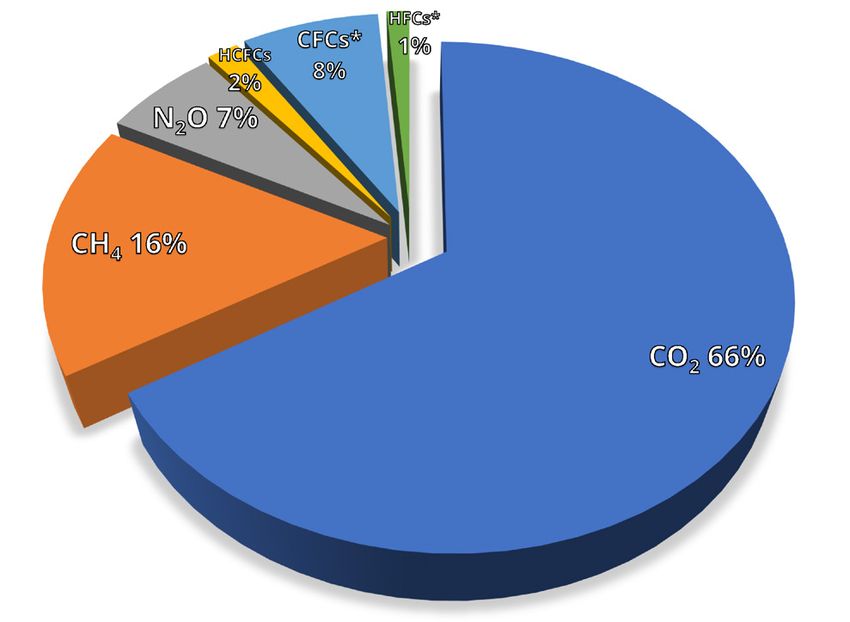
Figure 8. Globally averaged N2O mole fraction (a) and its growth
Figure 7. Globally averaged CH4 mole fraction (a) and its growth
                                                                         rate (b) from 1984 to 2020. Increases in successive annual
rate (b) from 1984 to 2020. Increases in successive annual means
                                                                         means are shown as shaded columns in (b). The red line in (a)
are shown as shaded columns in (b). The red line in (a) is the
                                                                         is the monthly mean with the seasonal variation removed; in
monthly mean with the seasonal variation removed; the blue dots
                                                                         this plot, the red line overlaps the blue dots and blue line that
and blue line in (a) depict the monthly averages. Observations
                                                                         depict the monthly averages. Observations from 105 stations
from 138 stations were used for this analysis.
                                                                         were used for this analysis.

Since 2007, atmospheric CH4 has been increasing, and in 2020             owing to the use of nitrogen fertilizers and manure, contributes
it reached 262% of the pre-industrial level due to increased             70% of all anthropogenic N2O emissions. This increase was
emissions from anthropogenic sources. Studies using GAW                  mainly responsible for the growth in the atmospheric burden
CH4 measurements indicate that increased CH4 emissions from              of N2O [19].
wetlands in the tropics and from anthropogenic sources at the
mid-latitudes of the northern hemisphere are the likely causes           Other greenhouse gases
of this recent increase.
                                                                         The stratospheric ozone-depleting CFCs, which are regulated
Recent studies have pointed to the short-term climate                    by the Montreal Protocol on Substances that Deplete the Ozone
benefits and cost-effectiveness of mitigating CH4 emissions              Layer, together with minor halogenated gases, account for
[17]. Some mitigation measures are presented in the                      approximately 11%(4) of the radiative forcing by LLGHGs. While
United Nations Environment Programme (UNEP) methane                      CFCs and most halons are decreasing, some HCFCs and HFCs,
assessment [18].                                                         which are also potent GHGs, are increasing at relatively rapid
                                                                         rates, although they are still low in abundance (at ppt(6) levels).
Nitrous oxide (N2O)                                                      The current observational network for CFCs is insufficient to
                                                                         determine important emission sources in a timely manner [20].
Nitrous oxide accounts for about 7%(4) of the radiative forcing by       Although at a similarly low abundance, SF6 is an extremely
LLGHGs. It is the third most important individual contributor to         potent LLGHG. It is produced by the chemical industry, mainly
the combined forcing. It is emitted into the atmosphere from both        as an electrical insulator in power distribution equipment. Its
natural sources (approximately 60%) and anthropogenic sources            current mole fraction is more than twice the level observed in
(approximately 40%), including oceans, soils, biomass burning,           the mid-1990s (Figure 9(a)).
fertilizer use and various industrial processes. The globally
averaged N2O mole fraction in 2020 reached 333.2 ± 0.1 ppb,              This Bulletin primarily addresses LLGHGs. Relatively short-
which is an increase of 1.2 ppb with respect to the previous             lived tropospheric ozone has a radiative forcing comparable
year (Figure 8) and 123% of the pre-industrial level (270 ppb).          to that of the halocarbons [21]. Many other pollutants, such as
The annual increase from 2019 to 2020 was higher than the                carbon monoxide (CO), nitrogen oxides and volatile organic
increase from 2018 to 2019 and higher than the mean growth               compounds, although not referred to as GHGs, have small
rate over the past 10 years (0.99 ppb yr-1). Global human-induced        direct or indirect effects on radiative forcing [9]. Aerosols
N2O emissions, which are dominated by nitrogen additions to              (suspended particulate matter) are short-lived substances
croplands, increased by 30% over the past four decades to 7.3            that alter the radiation budget. All the gases mentioned in this
(range: 4.2–11.4) teragrams of nitrogen per year. Agriculture,           Bulletin, as well as aerosols, are included in the observational

                                                                     7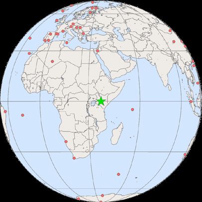
30                                                                                        600
                              (a) SF6 and halocarbons                                                                    (b) halocarbons
                         25                                                                                        500
   Mole fraction (ppt)

                                                                                             Mole fraction (ppt)
                                                                                                                                CFC-12
                         20                  HCFC-141b                                                             400

                         15                                                                                        300                     CFC-11
                                                        HCFC-142b

                         10                                                                                        200                                   HCFC-22
                                                                                                                                            CH3CCl3
                                             SF 6
                         5                                                                                         100                                      CCl4

                                                    HFC-152a
                                                                                                                         CFC-113              HFC-134a
                         0                                                                                            0
                              1995      2000        2005          2010   2015   2020                                  1975 1980 1985 1990 1995 2000 2005 2010 2015 2020
                                                           Year                                                                              Year

  Figure 9. Monthly mean mole fractions of SF6 and the most important halocarbons: (a) SF6 and lower mole fractions of halocarbons
  and (b) higher halocarbon mole fractions. For each gas, the number of stations used for the analysis was as follows: SF6 (88), CFC-11
  (23), CFC-12 (25), CFC-113 (22), CCl4 (22), CH3CCl3 (25), HCFC-141b (10), HCFC-142b (15), HCFC-22 (14), HFC-134a (11) and HFC-152a (10).

programme of GAW, with support from WMO Members and                                        Switzerland), Oksana Tarasova (WMO), Jocelyn Turnbull (GNS Science,
contributing networks [22].                                                                New Zealand/Cooperative Institute for Research in Environmental
                                                                                           Sciences, University of Colorado Boulder, United States of America),
Acknowledgements and links                                                                 Alex Vermeulen (ICOS ERIC/Lund University, Sweden).

Fifty-five WMO Members contributed CO2 and other GHG data to                               References
the GAW WDCGG. Approximately 40% of the measurement records
submitted to WDCGG were obtained at sites of the NOAA Global                               [1]                     Bennedsen, M., E. Hillebrand and S.J. Koopman, 2019: Trend
Monitoring Laboratory cooperative air-sampling network. For other                                                  analysis of the airborne fraction and sink rate of anthropogenically
networks and stations, see GAW Report No. 255 [23]. The Advanced                                                   released CO 2 . Biogeosciences, 16: 3651–3663, https://doi.
Global Atmospheric Gases Experiment also contributed observations                                                  org/10.5194/bg-16-3651-2019.
to this Bulletin. The GAW observational stations that contributed data                     [2]                     Ciavarella, A. et al., 2021: Prolonged Siberian heat of 2020 almost
to this Bulletin (see Figure 4) are included in the list of contributors                                           impossible without human influence. Climatic Change, 166: 9,
on the WDCGG web page (https://gaw.kishou.go.jp). They are also                                                    https://doi.org/10.1007/s10584-021-03052-w.
described in the GAW Station Information System, GAWSIS (http://                           [3]                     Jiang, L.Q., et al., 2019. Surface ocean pH and buffer capacity:
gawsis.meteoswiss.ch), supported by MeteoSwiss, Switzerland.                                                       past, present and future. Scientific Reports, 9: 18624, https://
The Bulletin is prepared under the oversight of the GAW Scientific                                                 doi.org/10.1038/s41598-019-55039-4.
Advisory Group on Greenhouse Gases.                                                        [4]                     Caesar, L. et al., 2021: Current Atlantic Meridional Overturning
                                                                                                                   Circulation weakest in last millennium. Nature Geoscience, 14:
                                                                                                                   118–120, https://doi.org/10.1038/s41561-021-00699-z.
Editorial board                                                                            [5]                     Manning, A. and R.F. Keeling, 2006: Global oceanic and land
                                                                                                                   biotic carbon sinks from the Scripps atmospheric oxygen flask
Alex Vermeulen (Integrated Carbon Observation System - European                                                    sampling network. Tellus B: Chemical and Physical Meteorology,
Research Infrastructure Consortium (ICOS ERIC)/Lund University,                                                    58(2): 95–116, https://doi.org/10.1111/j.1600-0889.2006.00175.x.
Sweden), Yousuke Sawa (Japan Meteorological Agency, WDCGG,                                 [6]                     GCOS, 2021: The Status of the Global Climate Observing System
Japan), Oksana Tarasova (WMO)                                                                                      2021: The GCOS Status Report, (GCOS-240), WMO, Geneva.
                                                                                           [7]                     Schibig, M.F., 2015: Carbon and oxygen cycle related atmospheric
                                                                                                                   measurements at the terrestrial background station Jungfraujoch.
Authors (in alphabetical order)                                                                                    PhD thesis, University of Bern.
                                                                                           [8]                     Butler, J.H. and S.A. Montzka, 2020: The NOAA Annual Greenhouse
Luana Basso (National Institute for Space Research, Brazil), Andy                                                  Gas Index (AGGI). NOAA, Earth System Research Laboratories,
Crotwell (NOAA Global Monitoring Laboratory and Cooperative                                                        Global Monitoring Laboratory, http://www.esrl.noaa.gov/gmd/
Institute for Research in Environmental Sciences, University of                                                    aggi/aggi.html.
Colorado Boulder, United States of America), Han Dolman (Vrije                             [9]                     IPCC, 2021: Climate Change 2021: The Physical Science Basis.
Universiteit Amsterdam, Netherlands), Luciana Gatti (National Institute                                            Contribution of Working Group I to the Sixth Assessment Report
for Space Research, Brazil), Christoph Gerbig (Max Planck Institute for                                            of the Intergovernmental Panel on Climate Change (V. Masson-
Biogeochemistry, Germany), David Griffith (University of Wollongong,                                               Delmotte et al., eds.). Cambridge University Press, https://www.
Australia), Bradley Hall (NOA A Global Monitoring Laboratory,                                                      ipcc.ch/report/sixth-assessment-report-working-group-i/.
United States of America), Armin Jordan (Max Planck Institute for                          [10]                    NOAA, Earth System Research Laboratories, Global Monitoring
Biogeochemistry, Germany), Paul Krummel (Commonwealth Scientific                                                   Laboratory, 2020: Trends in atmospheric carbon dioxide, http://
and Industrial Research Organisation, Australia), Markus Leuenberger                                               www.esrl.noaa.gov/gmd/ccgg/trends/.
(University of Bern, Switzerland), Zoë Loh (Commonwealth Scientific                        [11]                    Tsutsumi, Y. et al., 2009: Technical Report of Global Analysis
and Industrial Research Organisation, Australia), Sara Mikaloff-Fletcher                                           Method for Major Greenhouse Gases by the World Data
(GNS Science, Manaaki Whenua – Landcare Research, and University                                                   Center for Greenhouse Gases (WMO/ TD-No. 1473). GAW
of Waikato, New Zealand), Yousuke Sawa (Japan Meteorological                                                       Report No. 184. Geneva, WMO, https://library.wmo.int/index.
Agency, WDCGG, Japan), Michael Schibig (University of Bern,                                                        php?lvl=notice_display&id=12631.

                                                                                       8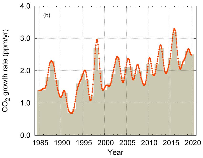
[12]   Hall, B.D. et al., 2021: Revision of the World Meteorological                        [26]   IPCC, 2019: 2019 Refinement to the 2006 IPCC Guidelines for
       Organization Global Atmosphere Watch (WMO/GAW) CO 2                                         National Greenhouse Gas Inventories, https://www.ipcc.ch/
       calibration scale. Atmospheric Measurement Techniques, 14:                                  report/2019-refinement-to-the-2006-ipcc-guidelines-for-national-
       3015–3032, https://doi.org/10.5194/amt-14-3015-2021.                                        greenhouse-gas-inventories/.
[13]   Le Quéré, C. et al., 2020: Temporary reduction in daily global                       [27]   Steinkamp, K. et al., 2017: Atmospheric CO2 observations and
       CO 2 emissions during the COVID-19 forced confinement.                                      models suggest strong carbon uptake by forests in New Zealand.
       Nature Climate Change, 10: 647–653, https://doi.org/10.1038/                                Atmospheric Chemistry and Physics, 17(1): 47–76, https://acp.
       s41558-020-0797-x.                                                                          copernicus.org/articles/17/47/2017/.
[14]   International Energy Agency, 2021: Global energy review:                             [28]   Gatti, L.V. et al., 2021: Amazonia as a carbon source linked to
       CO 2 emis sions in 2020, ht tp s: // w w w.iea.org /ar tic le s /                           deforestation and climate change. Nature, 595: 388–393, https://
       global-energy-review-co2-emissions-in-2020.                                                 doi.org/10.1038/s41586-021-03629-6.
[15]   Friedlingstein, P. et al., 2020: Global Carbon Budget 2020. Earth
       System Science Data, 12(4): 3269–3340, https://doi.org/10.5194/                      Contacts
       essd-12-3269-2020.
[16]   Saunois, M. et al., 2020: The Global Methane Budget 2000–                            World Meteorological Organization
       2017. Earth System Science Data, 12(3): 1561–1623, https://doi.                      Atmospheric Environment Research Division
       org/10.5194/essd-12-1561-2020.                                                       Science and Innovation Department
[17]   Nisbet, E.G. et al., 2020: Methane mitigation: methods to                            Geneva, Switzerland
       reduce emissions, on the path to the Paris Agreement.                                Email: gaw@wmo.int
       Reviews of Geophysics, 58(1): e2019RG000675, https://doi.                            Website: https://community.wmo.int/activity-areas/gaw
       org/10.1029/2019RG000675.
[18]   UNEP and Climate and Clean Air Coalition, 2021: Global Methane                       World Data Centre for Greenhouse Gases
       Assessment: Benefits and Costs of Mitigating Methane Emissions.                      Japan Meteorological Agency
       Nairobi, UNEP, https://www.unep.org/resources/report/global-                         Tokyo, Japan
       methane-assessment-benefits-and-costs-mitigating-methane-                            Email: wdcgg@met.kishou.go.jp
       emissions.                                                                           Website: https://gaw.kishou.go.jp
[19]   Tian, H. et al., 2020: A comprehensive quantification of global
       nitrous oxide sources and sinks. Nature, 586: 248–256, https://
       doi.org/10.1038/s41586-020-2780-0.
[20]   Weiss, R.F., A.R. Ravishankara and P.A. Newman, 2021: Huge
       gaps in detection networks plague emissions monitoring. Nature,
       595: 491–493, https://doi.org/10.1038/d41586-021-01967-z.
[21]   WMO, 2018: WMO Reactive Gases Bulletin: Highlights from the
       Global Atmosphere Watch Programme, No. 2, https://library.
       wmo.int/index.php?lvl=notice_display&id=20667#.YWCnpbj0njZ.                          Notes:
[22]   WMO, 2021: WMO Air Quality and Climate Bulletin, No. 1, https://                     (1) Mole fraction = the preferred expression for the abundance

       library.wmo.int/index.php?lvl=notice_display&id=21942.                                   (concentration) of a mixture of gases or fluids. In atmospheric
[23]   WMO, 2020: 20th WMO/IAEA Meeting on Carbon Dioxide, Other                                chemistry, the mole fraction is used to express the concentration
       Greenhouse Gases and Related Measurement Techniques                                      as the number of moles of a compound per mole of dry air.
       (GGMT-2019). GAW Report No. 255. Geneva, https://library.wmo.                        (2) ppm = the number of molecules of the gas per million (10 6 )

       int/doc_num.php?explnum_id=10353.                                                        molecules of dry air
[24]   Henne, S. et al., 2008: Mount Kenya Global Atmosphere Watch                          (3) ppb = the number of molecules of the gas per billion (109) molecules

       station (MKN): installation and meteorological characterization.                         of dry air
       Journal of Applied Meteorology and Climatology, 47(11): 2946–                        (4) This percentage is calculated as the relative contribution of the

       2962, https://doi.org/10.1175/2008jamc1834.1.                                            mentioned gas(es) to the increase in global radiative forcing
[25]   N e w Z e a l a n d M i n i s t r y f o r t h e En v i r o n m e n t , 2 0 21:           caused by all LLGHGs since 1750.
       New Zealand ’s Greenhouse Gas Inventor y 19 9 0 -2019                                (5) 1 GtCO = 1 billion (10 9) metric tons of carbon dioxide
                                                                                                        2
       Wellington, ht tps: //environment .gov t .nz /public ations /                        (6) ppt = the number of molecules of the gas per trillion (10 12 )

       new-zealands-greenhouse-gas-inventory-1990-2019/.                                        molecules of dry air

                                                                                        9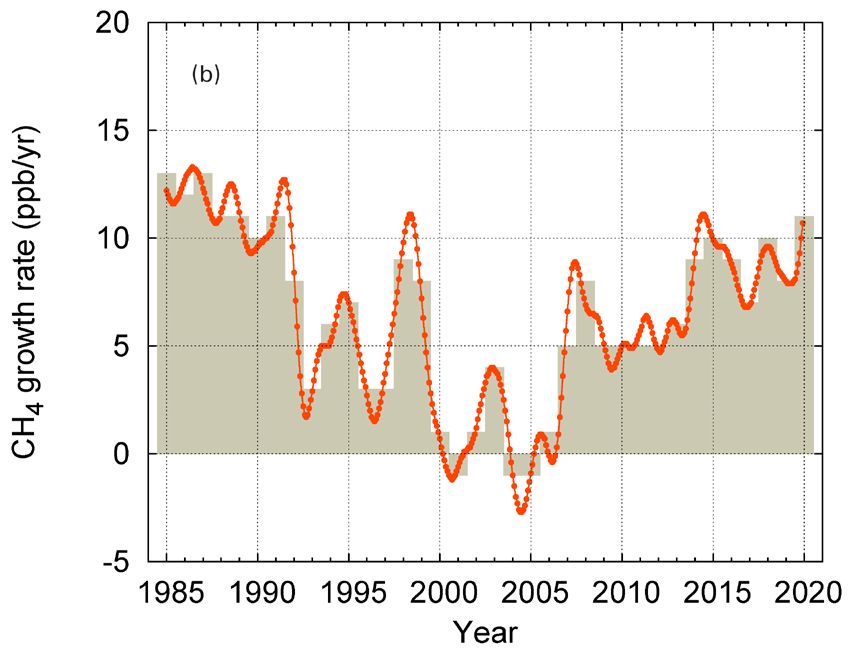
Selected greenhouse gas observatories

Mount Kenya (MKN)                                                         Barrow (BRW)

                                                                                                                                       Photo: NOAA
                                                                          Officially established in 1973, the Barrow Atmospheric
                                                                          Baseline Observatory (BRW) is NOAA’s northernmost station
                                                            Photo: WMO
                                                                          and the longest continuously operating atmospheric climate
                                                                          observatory in the Arctic. Located 8 km north-east of the city
                                                                          of Utqiaġvik (formerly Barrow), Alaska, BRW is purposely
                                                                          situated upwind of human habitation, in an isolated area
                                                                          which allows for the monitoring of air that has not been
The Mount Kenya GAW site (station identifier MKN) is located              affected by regional air pollution sources.
on the north-western slope of Mount Kenya close to the
Sirimon route and about 5 km south-west and 200 m below                   The original 74 m2 observatory building was built in 1973
Timau Hill [24]. It is operated by the Kenya Meteorological               and has hosted numerous long-term climate-related
Department, Nairobi. The mission of the station is to perform             measurements and campaign-style experiments during
long-term measurements of GHGs and aerosols in equatorial                 its tenure. After 47 years, the structure no longer met the
Africa and to assess the contribution of agricultural burning             needs of researchers and was replaced in 2020 with a new
and forest-clearing activities to the build-up of regional ozone.         273 m2 main building and support structures. The new
Mount Kenya is an isolated, almost conical mountain of                    facility includes a roof deck, a 30-m instrument tower, a
volcanic origin, which rises moderately from the surrounding              campaign science platform that can hold two 6-m metal
foreland (1 800–2 000 metres above sea level (m a.s.l)) to                shipping containers and a high-speed fibre connection
about 4 300 m a.s.l. The area has been protected since 1949               to the contiguous United States equipment that was
as part of Mount Kenya National Park and was designated                   transitioned to the new building in late 2020. Today, BRW
a World Heritage Site in 1997.                                            supports more than 200 measurements enabling research on
                                                                          atmospheric composition, climate, solar radiation, aerosols
The station was designed as a mobile two-container building               and stratospheric ozone.
that was completely equipped and taken into operation
in Germany by the Forschungszentrum Karlsruhe (FZK)
Institute for Meteorology and Climate Research–Atmospheric
Environmental Research. It was shipped as a whole unit to
Kenya. The station was officially inaugurated in October
1999. Cooperative flask sampling started with the NOAA
Global Monitoring Laboratory for the analysis of CO, CO2,
N2O, CH4, H2, SF6 and the isotopes of hydrogen and oxygen.
Instrument calibration is done biennially by the Swiss Federal
Laboratories for Materials Testing and Research (EMPA).
Power to the station is provided by a 26-km overland power
line passing through the tropical forest.

Location                                                                  Location
Country: Kenya                                                            Country: USA
Latitude: 0.0622° South                                                   Latitude: 71.323° North
Longitude: 37.2922° East                                                  Longitude: 156.611° West
Elevation: 3 644 m asl                                                    Elevation: 11 m asl
Time zone: Local time = UTC +3                                            Time zone: Local time = UTC – 9
                                                                                                                                                     JN 211402

                                                                         10
You can also read