A Competitive Deep Neural Network Approach for the ImageCLEFmed Caption 2020 Task
←
→
Page content transcription
If your browser does not render page correctly, please read the page content below
A Competitive Deep Neural Network Approach
                                               for the ImageCLEFmed Caption 2020 Task

                                                 Marimuthu Kalimuthu, Fabrizio Nunnari, and Daniel Sonntag

                                                     German Research Center for Artificial Intelligence (DFKI)
                                                    Saarland Informatics Campus, 66123 Saarbrücken, Germany
arXiv:2007.14226v3 [cs.CV] 22 Sep 2020

                                                   {marimuthu.kalimuthu,fabrizio.nunnari,daniel.sonntag}@dfki.de

                                               Abstract. The aim of ImageCLEFmed Caption task is to develop a
                                               system that automatically labels radiology images with relevant medical
                                               concepts. We describe our Deep Neural Network (DNN) based approach
                                               for tackling this problem. On the challenge test set of 3,534 radiology
                                               images, our system achieves an F1 score of 0.375 and ranks high, 12th
                                               among all systems that were successfully submitted to the challenge,
                                               whereby we only rely on the provided data sources and do not use any ex-
                                               ternal medical knowledge or ontologies, or pretrained models from other
                                               medical image repositories or application domains.

                                               Keywords: Medical Imaging, Concept Detection, Image Labeling, Multi-
                                               Label Classification, Deep Convolutional Neural Networks.

                                         1    Introduction

                                         ImageCLEF organises 4 main tasks for the 2020 edition with a global objec-
                                         tive of promoting the evaluation of technologies for annotation, indexing, and
                                         retrieval of visual data with the aim of providing information access to large col-
                                         lections of images in various usage scenarios and application domains, including
                                         medicine [4].
                                             Interpreting and summarizing the insights gained from medical images is a
                                         time-consuming task that involves highly trained experts and often represents a
                                         bottleneck in clinical diagnosis pipelines. Consequently, there is a considerable
                                         need for automatic methods that can approximate this mapping from visual in-
                                         formation to condensed textual descriptions. The more image characteristics are
                                         known, the more structured are the radiology scans and hence, the more efficient
                                         are the radiologists regarding interpretation, see https://www.imageclef.org/
                                         2020/medical/caption/ and [11].
                                             Recent years have witnessed tremendous advances in deep neural networks in
                                         terms of architectures, optimization algorithms, tooling and techniques for train-
                                         ing large networks, and handling multiple modalities (e.g., text, images, videos,
                                             Copyright © 2020 for this paper by its authors. Use permitted under Creative
                                         Commons License Attribution 4.0 International (CC BY 4.0). CLEF 2020, 22-25
                                         September 2020, Thessaloniki, Greece.
speech, etc.). In particular, deep convolutional neural networks have proved to
be extremely successful image encoders and have thus become the de facto stan-
dard for visual recognition [2,3,13]. We have been working on machine learning
problems in several medical application domains [14,15,16,17] in our projects, see
https://ai-in-medicine.dfki.de/. In this paper, we describe how we built a
competitive deep neural network approach based on these projects.
The rest of the paper is organized as follows. In Section 2, we formally de-
scribe the challenge and its goal. In Section 3, we present some statistics on
the dataset and explain the approach we adopted to tackle the challenge. In
Section 4, we describe the experiments that we conducted with different archi-
tectures and introduce a new loss function that addresses the sparsity problem
in ground truth labels. In Section 5, results are presented followed by a short
discussion. Finally, we summarize our work in Section 6 and discuss some future
directions.
2 The Challenge
The overarching goal of ImageCLEFmed Caption challenge is to assist medical
experts such as radiologists in interpreting and summarising information con-
tained in medical images. As a first step towards this goal, a simpler task would
be to detect as many key concepts as possible, with the goal that these concepts
can then be composed into comprehensible sentences, and eventually into med-
ical reports. For full details about the challenge, we refer the reader to Pelka et
al. [11].
The challenge has evolved over the years, since its first edition in 2017, to fo-
cus only on radiology images in this year’s version, and incorporating the lessons
learned from previous years. The aim of 2020 ImageCLEFmed Caption challenge
is to develop a system that would automatically assign medical concepts to ra-
diology images that were sorted into 7 different categories (see Table 1). More
concretely, given an image (I), the objective is to learn a function F that maps
I to a set of concepts (C1 , C2 , ..., CvI ) where vI is the number of concepts asso-
ciated with I. A peculiarity of this challenge is that v
k, where k is the total
number of unique labels.
F : I → (C1 , C2 , ..., CvI ) (1)
On the challenge data, the ground truth concepts are not known for images
in the test set. The only known constraint is that predictions of the test set must
be submitted with a maximum of 100 non-repeating concepts per image.
The performance of submissions to the challenge are evaluated on a withheld
test set of 3,534 radiology images using the F 1 score evaluation metric, which is
defined as the harmonic mean of precision and recall values.
precision ∗ recall
F1 = 2 ∗ (2)
precision + recallFirstly, the instance level F1 scores are computed using the predicted concepts
for images in the test set. Later, an average F1 score is computed over all images
in the test set using scikit-learn1 library’s default binary averaging method. This
yields the final F1 score for an accepted submission.
All registered teams are allowed for a maximum of 10 submissions. Successful
submissions and teams are then ranked based on the achieved F1 scores and
results are made publicly available.
3 Method
We provide information about the dataset and some analysis that we performed
on it during the exploratory phase. Then, we discuss our learning approach and
a suitable data preparation strategy for training our models.
3.1 Dataset
All participants are provided with ImageCLEFmed Caption dataset which is a
subset of the ROCO dataset [12]. It is a multi-modal, medical images dataset
containing radiology images that are each labelled with a set of medical concepts,
called as Concept Unique Identifiers (CUIs) in the literature. As common in
many challenges, the provided images are already split into train, validation,
and test sets. Images of the first two sets come with ground truth labels, while
the test set contains only images.
Table 1: Terminology used in the ROCO dataset.
Abbreviation Full form
DRAN DR Angiography
DRCO DR Combined modalities in One image
DRCT DR Computerized Tomography
DRMR DR Magenetic Resonance
DRPE DR Positron Emission Tomography
DRUS DR Ultrasound
DRXR DR X-Ray, 2D Tomography
Moreover, images in each of the splits are sorted into one of the 7 categories
as described in tables 1 and 2; such information can be inferred from the name
of the sub-directory containing the images. As we can observe from Table 2, the
images are not equally distributed across categories, indicating an imbalance in
the dataset. The DRCT category, which contains images captured using Com-
puterized Tomography (CT), has the highest representation, followed by X-ray
1
images (DRXR), while the least number of images (approximately 40 th of the
images in DRCT) are seen in DRCO category.
1
https://scikit-learn.org/stable/modules/generated/sklearn.metrics.f1_
score.htmlTable 2: Splits and statistics of the ImageCLEFmed Caption dataset.
Total Number of Images in the Category of
Split Total
DRAN DRCO DRCT DRMR DRPE DRUS DRXR
Train 4,713 487 20,031 11,447 502 8,629 18,944 64,753
Val 1,132 73 4,992 2,848 74 2,134 4,717 15,970
Test 325 49 1,140 562 38 502 918 3,534
Total 6,170 609 26,163 14,857 614 11,265 24,579 84,257
Despite having these category labels as a meta-information, we could not
leverage them during model training due to time constraints. Thus, the rela-
tionship between CUIs and image category labels is, for us, still uninvestigated.
Possibly, in a follow-up work we will investigate on how to exploit such meta-
information to improve classification performance of predictive models, for ex-
ample by using one of the metadata fusion strategies tested by the authors in [9].
3.2 Data Analysis
Here, we outline some insights that we gained after performing analysis on the
CUIs and the category labels meta-information. Furthermore, this section sheds
light on the imbalance in the dataset, which is a common problem in many
research domains.
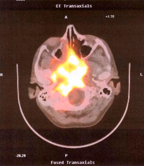
Figure 1 provides a conceptual representation of the input, viz. images paired
with relevant concepts. In this case, both images are labelled with four CUIs,
the descriptions of which are provided by Unified Medical Language System
(UMLS)2 terms. These terms are depicted in Figure 1 merely for the purpose
of understanding since the mapping of CUIs to UMLS terms is not part of the
provided dataset.
Figure 2 shows the frequencies of top 30 CUIs on the training split. Two CUIs
(C0040398, C0040405 ), which both occur around 20k times in the training set,
dominate this list and represent the concept “computer assisted tomography”.
Similar behavior is observed on the validation set (see Figure 3). However, the
frequencies of top 2 CUIs in this case are only around 4.6k.
Figure 4 depicts a histogram representation of the number of images and
the CUI counts on the training set. For instance, there are around 5,200 images
that have exactly two CUIs as ground truth labels. On the contrary, there are
only around 100 images that have exactly 50 CUIs as ground truth labels in the
provided training set. This histogram is truncated at CUI count 50 (x-axis) for
clarity and uncluttered representation.
In a similar manner, Figure 5 shows a histogram representation of the num-
ber of images and the CUI counts on the validation set. For instance, there are
around 1,300 images that have exactly two CUIs as ground truth labels. On the
contrary, there are only around 30 images that have exactly 50 CUIs as ground
2
https://www.nlm.nih.gov/research/umls/CUI UMLS Term (Concept) CUI UMLS Term
C2951888 set of bones of skull C0022742 knees
C0037303 set of bones of cranium C0043299 x-ray procedure
C0032743 tomogr positron emission C1260920 kneel
C0342952 increased basal metabolic rate C0030647 bone, patella
Fig. 1: Sample images & their CUIs from the train split.
truth labels in the validation set. This histogram is truncated at CUI count 50
(x-axis) for clarity and uncluttered representation.
On the combined training and validation set, there are 80,723 images and
907,718 non-unique CUIs. Among them, we counted 3,047 unique CUIs, which
were used to build the label space in our training objective (see Table 3).
Following Tsoumakas et al. [18], we compute the Label Cardinality (LC) on
the combined training and validation set, denoted as D, using the formula:
|D|
1 X
LC(D) = |Yi | (3)
|D| i=1
In a similar manner, we compute the Label Density (LD) using the following
formula:
|D|
1 X |Yi |
LD(D) = (4)
|D| i=1 |L|
where |L| is the number of unique labels in our multi-label classification
objective. The LC and LD scores on the combined training and validation sets
are 11.24 and 0.0037 respectively.CUI counts distribution for Train split
C0040398
C0040405
C0043299
C0024485
C0041618
C0002978
C0018792
C0021853
C0025066
C0227665
Concept Unique Identifiers (CUIs)
C0010709
C0030274
C0263833
C0030304
C0038351
C1322279
C0771711
C0070591
C0179620
C1441526
C0203379
C0013524
C0340305
C0024947
C0024687
C0007430 C0040398 : tomography, radionuclide computer-assisted
C0040405 : x-ray computer assisted tomography
C0004454 C0043299 : x-ray procedure
C0302148 C0024485 : tomogr nmr
C0041618 : medical sonography
C0013604 C0002978 : x-ray of the blood vessel
C0029053
0 1670 3340 5010 6680 8350 10020 11690 13360 15030 16700 18370 20040
Frequency of Concept Unique Identifiers (CUIs)
Fig. 2: Histogram of top 30 CUIs on the training split.
3.3 Data preparation
As a first step in formatting the labels, we convert CUIs associated with images
to a format that is suitable as input for neural network learning. Since our ob-
jective here is multi-label classification, we cannot use simple one-hot encoding,
as usually done in classification tasks, hence we apply a multi one-hot encoding.
An illustration of this representation can be found in Table 3. Specifically, we
sort the list of CUIs from the unique label set (k) in alphabetical order and use
the positions of CUIs in the sorted list to mark as 1 if a specific CUI is associated
with the image in question, else as 0. After this conversion step, the label set
for each image (I) is represented as a single multi one-hot vector of fixed size k,
which is equal to 3,047.
We used only the images from ImageCLEFmed Caption dataset and did not
use pre-training on external datasets, or utilize other modalities such as text
during model training.
For our experiments, we divided the validation set via random sampling into
two equally sized subsets, namely val1 and val2. We conducted our internalCUI counts distribution for Validation split
C0040398
C0040405
C0043299
C0024485
C0041618
C0002978
C0021853
C0030274
C0018792
C0227665
Concept Unique Identifiers (CUIs)
C0263833
C1322279
C0030304
C0025066
C0771711
C0010709
C0340305
C0011334
C0070591
C0302148
C0687028
C1441526
C0179620
C0013604
C0203379
C0013524 C0040398 : tomography, radionuclide computer-assisted
C0040405 : x-ray computer assisted tomography
C1140100 C0043299 : x-ray procedure
C0024687 C0024485 : tomogr nmr
C0041618 : medical sonography
C0038351 C0002978 : x-ray of the blood vessel
C0700185
0 417 834 1251 1668 2085 2502 2919 3336 3753 4170 4587
Frequency of Concept Unique Identifiers (CUIs)
Fig. 3: Histogram of top 30 CUIs on the validation split.
Table 3: Encoding CUIs using multi one-hot representation.
Multi One-Hot Encoding
Image
CUI01, CUI02, CUI03, . . . , CUI3047
ROCO2_CLEF _76012.jpg ...,0,1,0,0,1,0,0,0,1...
ROCO2_CLEF _05856.jpg ...,0,0,0,0,0,0,0,0,1...
ROCO2_CLEF _45763.jpg ...,0,1,0,0,1,0,1,0,0...
.. ..
. .
evaluations by always training pairs of models, first using val1 for validation
and val2 for testing, and then vice-versa. When results were promising, we then
submitted our predictions on the test set images by using the model trained with
first configuration. Training a third model, based on the validation on the full
development set would have been the ideal solution. However, this could not be
applied in our case because of time constraints.Histogram of CUI counts on the Train split
5201
4801
4401
4001
3601
Number of Images
3201
2801
2401
2001
1601
1201
801
401
1
1 2 3 4 5 6 7 8 9 10 11 12 13 14 15 16 17 18 19 20 21 22 23 24 25 26 27 28 29 30 31 32 33 34 35 36 37 38 39 40 41 42 43 44 45 46 47 48 49 50
Count of Concept Unique Identifiers (CUIs)
Fig. 4: Histogram of CUI counts vs. Images Count on the training set after
combining all of the 7 categories.
3.4 Learning Approach
The prediction problem for this challenge lays in the category of multi-label
classification [18]. It differs from most common classification problems in the
fact that each sample of the dataset is simultaneously associated with more
than one class from the ground truth label pool.
Technically, when addressing such a problem with deep neural networks, it
means that the final classification layer relies on multiple sigmoidal units rather
than a single softmax probability distribution. The last layer of the network
contains one sigmoidal unit for each of the target classes, and the association
with a true/false result is performed by thresholding the final sigmoid activation
value (usually at 0.5).
To address the challenge, we followed a classical transfer learning approach
starting from a Convolutional Neural Network (CNN) model pre-trained on an
image classification problem, namely ImageNet, because the pre-trained network
already offers the ability to detect basic image features, viz. edges, borders, and
corners. Then, the final classification stage of the network (i.e., all the layers
after the last convolutional layer) is substituted with randomly initialized fully
connected layers. Finally, the network is fitted for the new target training set.
In detail, we used VGG16 [13], ResNet50 [2], and DenseNet169 [3], all of
them pre-trained on ImageNet data used for ILSVRC [6]. An example configu-Histogram of CUI counts on the Validation split
1201
1101
1001
901
801
Number of Images
701
601
501
401
301
201
101
1
1 2 3 4 5 6 7 8 9 10 11 12 13 14 15 16 17 18 19 20 21 22 23 24 25 26 27 28 29 30 31 32 33 34 35 36 37 38 39 40 41 42 43 44 45 46 47 48 49 50
Count of Concept Unique Identifiers (CUIs)
Fig. 5: Histogram of CUI counts vs. Images Count on the validation set after
combining all of the 7 categories.
ration based on VGG16 is shown in listing 1.1. Layers from block1_conv1 to
block5_pool are pre-trained on ImageNet, and unlocked for further training.
Remaining layers, from flatten to predictions, are newly instantiated and
initialized randomly (where applicable). The final predictions layer is a dense
layer with 3,047 sigmoidal activation units (one per target class).
The system was developed in a Python environment using Keras deep learn-
ing framework [1] with TensorFlow [7] as the backend. For our experiments we
used a desktop machine equipped with an 8-core 9th -gen i7 CPU, 64GB RAM,
and NVIDIA RTX TITAN 24GB GPU memory.
4 Experiments
In this section, we describe our experimental procedure, model configuration, and
a variety of deep CNN architectures that we tried for achieving the multi-label
classification task.
Table 4 reports the results of the experiment we conducted throughout the
challenge. Because of time constraints, rather than running a grid search for the
best hyper-parameter values, we started from a reference configuration, already
successfully used in other past works [9,10].1 _________________________________________________________________
2 Layer ( type ) Output Shape Param #
3 =================================================================
4 input_1 ( InputLayer ) ( None , 227 , 227 , 3) 0
5 _________________________________________________________________
6 block1_conv1 ( Conv2D ) ( None , 227 , 227 , 64) 1792
7 _________________________________________________________________
8 block1_conv2 ( Conv2D ) ( None , 227 , 227 , 64) 36928
9 _________________________________________________________________
10 block1_pool ( MaxPooling2D ) ( None , 113 , 113 , 64) 0
11 _________________________________________________________________
12 [... 13 more layers ...]
13 _________________________________________________________________
14 block5_conv3 ( Conv2D ) ( None , 14 , 14 , 512) 2359808
15 _________________________________________________________________
16 block5_pool ( MaxPooling2D ) ( None , 7 , 7 , 512) 0
17 _________________________________________________________________
18 flatten ( Flatten ) ( None , 25088) 0
19 _________________________________________________________________
20 fc1 ( Dense ) ( None , 4096) 102764544
21 _________________________________________________________________
22 dropout_1 ( Dropout ) ( None , 4096) 0
23 _________________________________________________________________
24 fc2 ( Dense ) ( None , 4096) 16781312
25 _________________________________________________________________
26 dropout_2 ( Dropout ) ( None , 4096) 0
27 _________________________________________________________________
28 predictions ( Dense ) ( None , 3047) 12483559
29 =================================================================
30 Total params : 146 ,744 ,103
31 Trainable params : 146 ,744 ,103
32 Non - trainable params : 0
33 _________________________________________________________________
Listing 1.1: An excerpt of the VGG16 architecture used for the multi-label
classification task.
Together with the base architecture used for convolution (CNN arch) we
report: (res) the resolution in pixels of the input images of equal height and
width, (aug) the data augmentation strategy, (fc layers) the configuration of
final fully-connected stage of the CNN architectures, (do) the dropout value after
each fully connected layer, (bs) the batch size used for training, (loss func) the
loss function used for optimization, (lr-red) the learning rate reduction strategy
(reduction factor/patience/monitored metric). Additionally, we report the best
training epoch, based on an early stopping criteria by monitoring the F1 score on
the validation set. The last three columns report the F1 scores achieved on the
two internal cross-validation sets and finally on the AIcrowd3 online submission
platform.
Other training parameters, common to all configurations are: NAdam opti-
mizer, learning rate = 1e-5, and schedule decay 0.9. All images were scaled to
the input resolution of the CNN using nearest filtering, without any cropping.
In the following, we report on the evolution of our tests and obtained results.
3
https://www.aicrowd.com/challenges/imageclef-2020-caption-concept-
detectionTable 4: The list of experiments conducted for the challenge.
# CNN arch res aug. fc do bs loss lr-red. test1 test2 score
(px) layers func ep F1 ep F1 F1
1 VGG16 227 none 2x2k 0.5 32 bce 0.2/3/loss 12 0.333 22 0.335
2 VGG16 227 none 2x4k 0.5 32 bce 0.2/3/loss 25 0.346 26 0.336
3 VGG16 227 hflip 2x4k 0.5 32 bce 0.2/5/f1 9 0.3475 9 0.3455 0.363
4 VGG16 450 hflip 2x4k 0.5 24 bce 0.2/5/f1 n/a crash 6 0.3417
5 ResNet50 224 hflip 2x4k 0.5 16 bce nothing 3 0.3484 3 0.3487 0.365
6 DenseNet169 224 none 2x4k 0.5 32 bce nothing 8 0.3495 10 0.3450
7 DenseNet169 224 hflip 2x4k 0.5 32 bce nothing 5 0.3500 4 0.3463 0.360
8 VGG16 227 hflip 3x4k 0.5 32 bce 0.2/5/f1 13 0.3465 14 0.3433
9 VGG16 227 hflip 2x4k 0.5 48 F 1 ∗ bce 0.2/5/f1 11 0.3604 7 0.3606 0.374
10 VGG16 227 hflip 2x4k 0.5 48 F 1 + bce 0.2/5/f1 14 0.3636 12 0.3632
Experiments 1-4: VGG16 baseline We started with (1) a VGG16 archi-
tecture, pretrained on ImageNet, with the last two fully connected (FC) layers
configured with n=2048 nodes, each followed by a dropout layer with the dropout
probability p set to 0.5.
(2) We observed an increase in performance by increasing the size of the FC
layers to 4096 nodes.
From the first two experiments, it was evident how the loss value (based on
binary cross-entropy) could not be effectively used to monitor the validation. The
ground truth of each sample, a vector of size 3,047, contains on average about 11
concepts per image (see Section 3.2), and only a few images contain more than
50 concepts. Hence, the ground truth matrix is very sparse. As a consequence,
the loss function quickly stabilizes into a plateau, as does the accuracy, which
saturates to values above 0.9966 after the first epoch. Hence, to better handle
early stopping, we implemented a training-time computation of the F1 score.
(3) A further improvement was observed by applying a 2X data augmentation
of the input dataset. Each image is provided to the training procedure both
as-it-is and flipped horizontally. At the same time, learning rate reduction was
applied by monitoring F1 scores on the validation set, rather than the loss values.
However, increasing the learning rate happens only after an overfitting occurs.
This configuration led to an online evaluation score of 0.363. Figure 6 shows the
evolution of loss values and F1 scores over epochs during model training.
(4) We tried to improve the performance by increasing the size of input
images to 450x450 pixels, which forced a reduction of the batch size to 24. We
could not observe any significant improvement in the accuracy, suggesting that
higher image resolutions do not provide useful details for label selection in our
case.
Experiments 5-7: more powerful CNN architectures By using deeper
CNN architectures, we could observe a slight improvement in the test accuracy.
Indeed, the ResNet50 architecture (5) led to an F1 score of 0.365 in the onlineLoss (Binary cross-entropy) F1 score
0.034 0.355
0.35
0.032
0.345
0.03 0.34
0.028 0.335
0.33
0.026
0.325
0.024 0.32
0.022 0.315
0.31
0.02
0.305
0.018 0.3
-5 0 5 10 15 20 25 3 -5 0 5 10 15 20 25 3
Fig. 6: Plots of the metrics computed on the validation set during training: (left)
binary cross-entropy and (right) F1 score. Here, epochs are counted from 0. The
best validation results are achieved at epoch 9, then the model starts overfitting.
evaluation. The DenseNet169 architecture (6-7) led to higher test values, but
the online evaluation was slightly lower (0.360) than the ResNet50 version.
Experiment 8: more layers In order to increase the overall performance,
we tried to increase the number of FC layers to 3x4k (8). However, taking as
reference the performance of configuration (3), we could not observe a significant
improvement by introducing an additional 4k FC layer to the classification stage.
Experiments 9-10: a new loss function To further improve performance,
we decided to directly optimize for the F1 score evaluation metric. Notice that
the F1 score used in the ImageCLEF challenge is computed as an average F1
over the samples (and not over the labels, as more often found in online code
repositories4,5 ).
We implemented a loss function F 1 = 1 − sF 1, where sF 1 is called the “soft
F1 score”. The sF 1 is a differentiable version of the F1 function that computes
true positives, false positives, and false negatives as continuous sum of likelihood
values, without applying any thresholding to round the probabilities to 0 or 1.
The implementation of F 1 is shown in listing 1.2.
Experiments using the F 1 loss function could not converge. Likely, the prob-
lem is due to the fact that the F 1 loss lies in the range [0, 1]. As such, the
gradient search space can be abstractly seen as a huge plateau, just below 1.0,
with a solitary hole in the middle that quickly converges to the global minimum.
At the same level of abstraction, we can visualize the binary cross-entropy bce
search space as a wide bag, with a large flat surface, just above 0. It is easy to
reach the bottom of the bag, i.e., reach a very high binary accuracy due to the
sparsity of the labeling, but then we see a very mild slope towards the global
4
https://towardsdatascience.com/the-unknown-benefits-of-using-a-soft-
f1-loss-in-classification-systems-753902c0105d
5
https://www.kaggle.com/rejpalcz/best-loss-function-for-f1-score-
metric1 def l os s _1 _m i nu s_ f 1 ( y_true , y_pred ) :
2
3 import keras . backend as K
4 import tensorflow as tf
5
6 # The following is not d iffere ntiabl e .
7 # Round the prediction to 0 or 1 (0.5 threshold )
8 # y_pred = K . round ( y_pred )
9 # By commenting , we implement what is called soft - F1 .
10
11 # Compute precision and recall .
12 tp = K . sum ( K . cast ( y_true * y_pred , ’ float ’) , axis = -1)
13 # tn = K . sum ( K . cast ((1 - y_true ) * (1 - y_pred ) , ’ float ’) , axis = -1)
14 fp = K . sum ( K . cast ((1 - y_true ) * y_pred , ’ float ’) , axis = -1)
15 fn = K . sum ( K . cast ( y_true * (1 - y_pred ) , ’ float ’) , axis = -1)
16
17 p = tp / ( tp + fp + K . epsilon () )
18 r = tp / ( tp + fn + K . epsilon () )
19
20 # Compute F1 and return the loss .
21 f1 = 2 * p * r / ( p + r + K . epsilon () )
22 f1 = tf . where ( tf . is_nan ( f1 ) , tf . zeros_like ( f1 ) , f1 )
23 return 1 - K . mean ( f1 )
Listing 1.2: Python implementation of the soft-F1 based loss function for the
Keras environment with TensorFlow backend.
1 def l o s s _ 1 m f 1 _ b y _ b c e ( y_true , y_pred ) :
2 import keras . backend as K
3
4 loss_f1 = l o ss _1 _ mi nu s _f 1 ( y_true , y_pred )
5 bce = K . b i n a r y _ c r o s s e n t r o p y ( target = y_true , output = y_pred , from_logits =
False )
6
7 return loss_f1 * bce
Listing 1.3: Python implementation of the loss function combining soft-F1 score
with binary cross-entropy.
minimum at its center.
Our intuition is that by combining (multiplying or adding) F 1 and bce results
in a search space where F 1 does not affect the identification of inside of the
bag, and at the same time helps with the identification of the F 1’s and bce’s
common global minimum. The implementation of the F 1 ∗ bce loss function is
straightforward and is presented in listing 1.3.
(9) An experiment using VGG16 confirms that the loss function F 1 ∗ bce
leads to better results with 0.3604/0.3606 on our tests. This is the configuration
that performed best in the online submission (0.374).
Further experiments, e.g., using ResNet50, could not be submitted to the
challenge due to time constraints. However, (10) an internal test using VGG16Table 5: F1 scores for submissions by our team ‘iml’ .
AIcrowd Submission Run F1 Score Rank
imageclefmed2020-test-vgg16-f1-bce-nomissing-iml.txt 0.374525478882926 12
imageclefmed2020-test-vgg16-f1-bce-iml.txt 0.374402134956526 13
imageclefmed2020-test-resnet50-iml.txt 0.365168555515581 17
imageclefmed2020-test-vgg16-iml.txt 0.363067945861981 18
imageclefmed2020-test-densenet169-iml.txt 0.360156086299303 19
in combination with the F 1 + bce loss function, led to the best performance in
our internal evaluation (0.3636/0.3632).
5 Results and Discussion
The results of our experiments for the ImageCLEFmedical 2020 challenge can
be summarized as follows.
The task of concept detection can be modeled as a multi-labeling problem
and solved by a transfer learning approach where deep CNNs pretrained on
real-world images can be fine-tuned on the target dataset. The multi-labeling is
technically addressed by using a sigmoid activation function on the output layer
and a label selection by thresholding. A good configuration consists of a VGG16
deep CNN architecture followed by two fully connected layers of 4096 nodes,
each followed by a dropout layer with probability p set to 0.5. Augmenting
the training set with horizontally flipped images increases accuracy and also
reduces the number of epochs needed for training. Increasing the resolution of
input images does not prove to be useful, while better results are achieved by
substituting the convolution stage with a deeper CNN architecture (ResNet50).
We noticed that the learning rate reduction has never helped in improving the
results.
Using the standard binary cross-entropy loss function leads to competitive
results, which significantly increases when it is combined with a soft-F1 score
computation. It is worth noticing that when using solely the soft-F1 score as a
loss function, the network could not converge and this problem needs further
investigation.
In total, we made five online submissions to the challenge. Table 5 presents
the F1 scores achieved on the withheld test set and the overall ranking of our
team (iml ) out of 47 successful submissions, as reported by the challenge or-
ganizers. In addition, it is worth mentioning that the difference in F1 scores
between our best submission and the system that achieved the highest score in
the challenge is 0.0195. What percentage of test set images on which our model
still needs to achieve correct labels to bridge this gap needs further investigation.6 Conclusion and Future Directions
In this work we have proposed a deep convolutional neural network based ap-
proach for concept detection in radiology images. Our best performance (12th
position) is achieved by implementing a new loss function whereby we combined
the widely used binary cross-entropy loss together with a differentiable version
of the F1 score evaluation metric.
Still several aspects could be investigated to improve the achieved results. For
instance, as we can observe from the CUI distribution plots, there is an imbalance
in the dataset. Consequently the model is biased towards predicting the concepts
associated with over-represented samples. Our future work will focus on the
approaches to combat such type of biases. A straightforward approach would
be to undersample the over-represented samples using a query strategy that
maximizes informativeness of chosen samples. Such a strategy showed promising
results for incremental domain adaptation task in neural machine translation [5].
Furthermore, we did not make use of the existing categorization of the images
in 7 sub-sets. A straightforward idea would be to train 7 different models, one
per category, and rely on their ensemble for a final global classification result.
Alternatively, the class identifier might be used as additional metadata informa-
tion, concatenated to the images’ internal features representation in the CNN,
and fed to a further shallow neural network for improved classification (see [9]).
Another promising direction to look would be to consider further trends in the
integration of vision and language research [8].
References
1. Keras Special Interest Group. Keras. https://keras.io/.
2. Kaiming He, Xiangyu Zhang, Shaoqing Ren, and Jian Sun. Deep residual learning
for image recognition. In 2016 IEEE Conference on Computer Vision and Pattern
Recognition, CVPR 2016, Las Vegas, NV, USA, June 27-30, 2016, pages 770–778.
IEEE Computer Society, 2016.
3. Gao Huang, Zhuang Liu, Laurens van der Maaten, and Kilian Q. Weinberger.
Densely connected convolutional networks. In 2017 IEEE Conference on Computer
Vision and Pattern Recognition, CVPR 2017, Honolulu, HI, USA, July 21-26,
2017, pages 2261–2269. IEEE Computer Society, 2017.
4. Bogdan Ionescu, Henning Müller, Renaud Péteri, Asma Ben Abacha, Vivek
Datla, Sadid A. Hasan, Dina Demner-Fushman, Serge Kozlovski, Vitali Liauchuk,
Yashin Dicente Cid, Vassili Kovalev, Obioma Pelka, Christoph M. Friedrich, Alba
García Seco de Herrera, Van-Tu Ninh, Tu-Khiem Le, Liting Zhou, Luca Piras,
Michael Riegler, Pål Halvorsen, Minh-Triet Tran, Mathias Lux, Cathal Gurrin,
Duc-Tien Dang-Nguyen, Jon Chamberlain, Adrian Clark, Antonio Campello, Dim-
itri Fichou, Raul Berari, Paul Brie, Mihai Dogariu, Liviu Daniel Ştefan, and Mi-
hai Gabriel Constantin. Overview of the ImageCLEF 2020: Multimedia retrieval in
medical, lifelogging, nature, and internet applications. In Experimental IR Meets
Multilinguality, Multimodality, and Interaction, volume 12260 of Proceedings of
the 11th International Conference of the CLEF Association (CLEF 2020), Thessa-
loniki, Greece, September 22-25 2020. LNCS Lecture Notes in Computer Science,
Springer.5. Marimuthu Kalimuthu, Michael Barz, and Daniel Sonntag. Incremental domain
adaptation for neural machine translation in low-resource settings. In Wassim El-
Hajj, Lamia Hadrich Belguith, Fethi Bougares, Walid Magdy, and Imed Zitouni,
editors, Proceedings of the Fourth Arabic Natural Language Processing Workshop,
WANLP@ACL 2019, Florence, Italy, August 1, 2019, pages 1–10. Association for
Computational Linguistics, 2019.
6. Alex Krizhevsky, Ilya Sutskever, and Geoffrey E Hinton. ImageNet Classification
with Deep Convolutional Neural Networks. In F. Pereira, C. J. C. Burges, L. Bot-
tou, and K. Q. Weinberger, editors, Advances in Neural Information Processing
Systems 25, pages 1097–1105. Curran Associates, Inc., 2012.
7. Martín Abadi, Ashish Agarwal, Paul Barham, Eugene Brevdo, Zhifeng Chen, Craig
Citro, Greg S. Corrado, Andy Davis, Jeffrey Dean, Matthieu Devin, Sanjay Ghe-
mawat, Ian Goodfellow, Andrew Harp, Geoffrey Irving, Michael Isard, Yangqing
Jia, Rafal Jozefowicz, Lukasz Kaiser, Manjunath Kudlur, Josh Levenberg, Dande-
lion Mané, Rajat Monga, Sherry Moore, Derek Murray, Chris Olah, Mike Schuster,
Jonathon Shlens, Benoit Steiner, Ilya Sutskever, Kunal Talwar, Paul Tucker, Vin-
cent Vanhoucke, Vijay Vasudevan, Fernanda Viégas, Oriol Vinyals, Pete Warden,
Martin Wattenberg, Martin Wicke, Yuan Yu, and Xiaoqiang Zheng. TensorFlow:
Large-Scale Machine Learning on Heterogeneous Systems. 2015.
8. Aditya Mogadala, Marimuthu Kalimuthu, and Dietrich Klakow. Trends in inte-
gration of vision and language research: A survey of tasks, datasets, and methods.
CoRR, abs/1907.09358, 2019.
9. Fabrizio Nunnari, Chirag Bhuvaneshwara, Abraham Obinwanne Ezema, and
Daniel Sonntag. A study on the fusion of pixels and patient metadata in CNN-based
classification of skin lesion images. In International IFIP Cross Domain Conference
for Machine Learning and Knowledge Extraction (CD-MAKE). Springer, August
2020.
10. Fabrizio Nunnari and Daniel Sonntag. A CNN toolbox for skin cancer classification.
arXiv:1908.08187 [cs, eess], August 2019. arXiv: 1908.08187.
11. Obioma Pelka, Christoph M Friedrich, Alba García Seco de Herrera, and Henning
Müller. Overview of the ImageCLEFmed 2020 concept prediction task: Medical
image understanding. In CLEF2020 Working Notes, CEUR Workshop Proceedings,
Thessaloniki, Greece, September 22-25 2020. CEUR-WS.org.
12. Obioma Pelka, Sven Koitka, Johannes Rückert, Felix Nensa, and Christoph M
Friedrich. Radiology objects in context (roco): A multimodal image dataset. In
Intravascular Imaging and Computer Assisted Stenting and Large-Scale Annotation
of Biomedical Data and Expert Label Synthesis, pages 180–189. Springer, 2018.
13. Karen Simonyan and Andrew Zisserman. Very deep convolutional networks for
large-scale image recognition. In Yoshua Bengio and Yann LeCun, editors, 3rd
International Conference on Learning Representations, ICLR 2015, San Diego,
CA, USA, May 7-9, 2015, Conference Track Proceedings, 2015.
14. Daniel Sonntag. AI in Medicine, Covid-19 and Springer Nature’s Open Access
Agreement. KI, 34(2):123–125, 2020.
15. Daniel Sonntag, Fabrizio Nunnari, and Hans-Jürgen Profitlich. The Skincare
project, an interactive deep learning system for differential diagnosis of malignant
skin lesions. Technical Report. CoRR, abs/2005.09448, 2020.
16. Daniel Sonntag and Hans-Jürgen Profitlich. An architecture of open-source tools
to combine textual information extraction, faceted search and information visual-
isation. Artificial Intelligence in Medicine, 93:13–28, 2019.17. Daniel Sonntag, Volker Tresp, Sonja Zillner, Alexander Cavallaro, Matthias Ham-
mon, André Reis, Peter A. Fasching, Martin Sedlmayr, Thomas Ganslandt, Hans-
Ulrich Prokosch, Klemens Budde, Danilo Schmidt, Carl Hinrichs, Thomas Wit-
tenberg, Philipp Daumke, and Patricia G. Oppelt. The clinical data intelligence
project - A smart data initiative. Informatik Spektrum, 39(4):290–300, 2016.
18. Grigorios Tsoumakas and Ioannis Katakis. Multi-Label Classification: An
Overview. International Journal of Data Warehousing and Mining, 3(3):1–13, July
2007.You can also read