Restoring An Image Taken Through a Window Covered with Dirt or Rain
←
→
Page content transcription
If your browser does not render page correctly, please read the page content below
Restoring An Image Taken Through a Window Covered with Dirt or Rain

                                 David Eigen Dilip Krishnan Rob Fergus
                      Dept. of Computer Science, Courant Institute, New York University
                                           {deigen,dilip,fergus}@cs.nyu.edu

                         Abstract

   Photographs taken through a window are often compro-
mised by dirt or rain present on the window surface. Com-
mon cases of this include pictures taken from inside a ve-
hicle, or outdoor security cameras mounted inside a pro-
tective enclosure. At capture time, defocus can be used to
remove the artifacts, but this relies on achieving a shallow
depth-of-field and placement of the camera close to the win-
dow. Instead, we present a post-capture image processing
solution that can remove localized rain and dirt artifacts
from a single image. We collect a dataset of clean/corrupted
image pairs which are then used to train a specialized form
of convolutional neural network. This learns how to map
corrupted image patches to clean ones, implicitly capturing
the characteristic appearance of dirt and water droplets in
natural images. Our models demonstrate effective removal              Figure 1. A photograph taken through a glass pane covered in rain,
of dirt and rain in outdoor test conditions.                          along with the output of our neural network model, trained to re-
                                                                      move this type of corruption. The irregular size and appearance of
                                                                      the rain makes it difficult to remove with existing methods. This
                                                                      figure is best viewed in electronic form.
1. Introduction
   There are many situations in which images or video                 the glass and using a large aperture to produce small depth-
might be captured through a window. A person may be                   of-field. However, in practice it can be hard to move the
inside a car, train or building and wish to photograph the            camera sufficiently close, and aperture control may not be
scene outside. Indoor situations include exhibits in muse-            available on smartphone cameras or webcams. Correspond-
ums displayed behind protective glass. Such scenarios have            ingly, many shots with smartphone cameras through dirty or
become increasingly common with the widespread use of                 rainy glass still have significant artifacts, as shown in Fig. 9.
smartphone cameras. Beyond consumer photography, many                     In this paper we instead restore the image after capture,
cameras are mounted outside, e.g. on buildings for surveil-           treating the dirt or rain as a structured form of image noise.
lance or on vehicles to prevent collisions. These cameras             Our method only relies on the artifacts being spatially com-
are protected from the elements by an enclosure with a                pact, thus is aided by the rain/dirt being in focus — hence
transparent window.                                                   the shots need not be taken close to the window.
   Such images are affected by many factors including re-                 Image denoising is a very well studied problem, with
flections and attenuation. However, in this paper we address          current approaches such as BM3D [3] approaching theo-
the particular situation where the window is covered with             retical performance limits [13]. However, the vast majority
dirt or water drops, resulting from rain. As shown in Fig. 1,         of this literature is concerned with additive white Gaussian
these artifacts significantly degrade the quality of the cap-         noise, quite different to the image artifacts resulting from
tured image.                                                          dirt or water drops. Our problem is closer to shot-noise re-
   The classic approach to removing occluders from an im-             moval, but differs in that the artifacts are not constrained to
age is to defocus them to the point of invisibility at the time       single pixels and have characteristic structure. Classic ap-
of capture. This requires placing the camera right up against         proaches such as median or bilateral filtering have no way

                                                                  1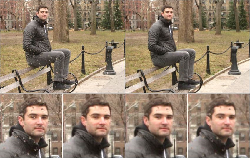
of leveraging this structure, thus cannot effectively remove          Several papers explore the removal of rain from images.
the artifacts (see Section 5).                                     Garg and Nayar [7] and Barnum et al. [1] address air-
    Our approach is to use a specialized convolutional neural      borne rain. The former uses defocus, while the latter uses
network to predict clean patches, given dirty or clean ones        frequency-domain filtering. Both require video sequences
as input. By asking the network to produce a clean output,         rather than a single image, however. Roser and Geiger
regardless of the corruption level of the input, it implicitly     [17] detect raindrops in single images; although they do not
must both detect the corruption and, if present, in-paint over     demonstrate removal, their approach could be paired with
it. Integrating both tasks simplifies and speeds test-time op-     a standard inpainting algorithm. As discussed above, our
eration, since separate detection and in-painting stages are       approach combines detection and inpainting.
avoided.                                                              Closely related to our application is Gu et al. [9], who
    Training the models requires a large set of patch pairs        show how lens dust and nearby occluders can be removed,
to adequately cover the space inputs and corruption, the           but their method requires extensive calibration or a video se-
gathering of which was non-trivial and required the devel-         quence, as opposed to a single frame. Wilson et al. [19] and
opment of new techniques. However, although training is            Zhou and Lin [22] demonstrate dirt and dust removal. The
somewhat complex, test-time operation is simple: a new             former removes defocused dust for a Mars Rover camera,
image is presented to the neural network and it directly out-      while the latter removes sensor dust using multiple images
puts a restored image.                                             and a physics model.
1.1. Related Work                                                  2. Approach
   Learning-based methods have found widespread use in                 To restore an image from a corrupt input, we predict a
image denoising, e.g. [23, 14, 16, 24]. These approaches           clean output using a specialized form of convolutional neu-
remove additive white Gaussian noise (AWGN) by building            ral network [12]. The same network architecture is used
a generative model of clean image patches. In this paper,          for all forms of corruption; however, a different network is
however, we focus on more complex structured corruption,           trained for dirt and for rain. This allows the network to tai-
and address it using a neural network that directly maps cor-      lor its detection capabilities for each task.
rupt images to clean ones; this obviates the slow inference
procedures used by most generative models.                         2.1. Network Architecture
   Neural networks have previously been explored for de-               Given a noisy image x, our goal is to predict a clean
noising natural images, mostly in the context of AWGN,             image y that is close to the true clean image y ∗ . We
e.g. Jain and Seung [10], and Zhang and Salari [21]. Al-           accomplish this using a multilayer convolutional network,
gorithmically, the closest work to ours is that of Burger          y = F (x). The network F is composed of a series of layers
et al. [2], which applies a large neural network to a range of     Fl , each of which applies a linear convolution to its input,
non-AWGN denoising tasks, such as salt-and-pepper noise            followed by an element-wise sigmoid (implemented using
and JPEG quantization artifacts. Although more challeng-           hyperbolic tangent). Concretely, if the number of layers in
ing than AWGN, the corruption is still significantly easier        the network is L, then
than the highly variable dirt and rain drops that we address.
Furthermore, our network has important architectural dif-          F0 (x)     = x
ferences that are crucial for obtaining good performance on        Fl (x)     = tanh(Wl ∗ Fl−1 (x) + bl ),             l = 1, ..., L − 1
these tasks.                                                                     1
   Removing localized corruption can be considered a form           F (x)     =    (WL ∗ FL−1 (x) + bL )
                                                                                m
of blind inpainting, where the position of the corrupted re-
gions is not given (unlike traditional inpainting [5]). Dong       Here, x is the RGB input image, of size N × M × 3. If
et al. [4] show how salt-and-pepper noise can be removed,          nl is the output dimension at layer l, then Wl applies nl
but the approach does not extend to multi-pixel corruption.        convolutions with kernels of size pl × pl × nl−1 , where pl
Recently, Xie et al. [20] showed how a neural network can          is the spatial support. bl is a vector of size nl containing the
perform blind inpainting, demonstrating the removal of text        output bias (the same bias is used at each spatial location).
synthetically placed in an image. This work is close to ours,          While the first and last layer kernels have a nontrivial
but the solid-color text has quite different statistics to natu-   spatial component, we restrict the middle layers (2 ≤ l ≤
ral images, thus is easier to remove than rain or dirt which       L − 1) to use pl = 1, i.e. they apply a linear map at each
vary greatly in appearance and can resemble legitimate im-         spatial location. We also element-wise divide the final out-
age structures. Jancsary et al. [11] denoise images with a         put by the overlap mask1 m to account for different amounts
Gaussian conditional random field, constructed using deci-         of kernel overlap near the image boundary. The first layer
sion trees on local regions of the input; however, they too           1 m = 1 ∗ 1 , where 1 is a kernel of size p × p filled with ones,
                                                                                K    I         K                     L     L
consider only synthetic corruptions.                               and 1I is a 2D array of ones with as many pixels as the last layer input.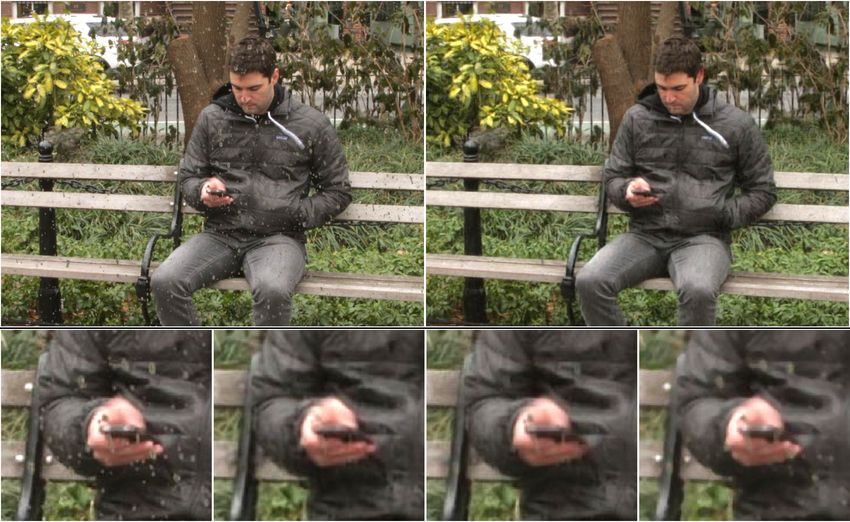
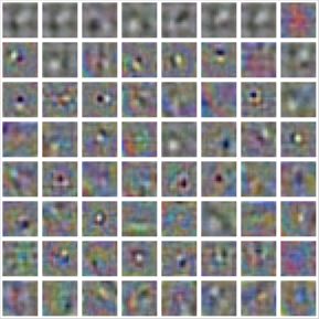
Figure 2. A subset of rain model network weights, sorted by l2 -
norm. Left: first layer filters which act as detectors for the rain
drops. Right: top layer filters used to reconstruct the clean patch. (a) (b) (c)
Figure 3. Denoising near a piece of noise. (a) shows a 64 × 64 im-
uses a “valid” convolution, while the last layer uses a “full” age region with dirt occluders (top), and target ground truth clean
(these are the same for the middle layers since their kernels image (bottom). (b) and (c) show the results obtained using non-
have 1 × 1 support). convolutional and convolutionally trained networks, respectively.
In our system, the input kernels’ support is p1 = 16, and The top row shows the full output after averaging. The bottom
the output support is pL = 8. We use two hidden layers (i.e. row shows the signed error of each individual patch prediction for
all 8 × 8 patches obtained using a sliding window in the boxed
L = 3), each with 512 units. As stated earlier, the middle
area, displayed as a montage. The errors from the convolutionally-
layer kernel has support p2 = 1. Thus, W1 applies 512
trained network (c) are less correlated with one another compared
kernels of size 16 × 16 × 3, W2 applies 512 kernels of size to (b), and cancel to produce a better average.
1 × 1 × 512, and W3 applies 3 kernels of size 8 × 8 × 512.
Fig. 2 shows examples of weights learned for the rain data.
2.3. Effect of Convolutional Architecture
2.2. Training A key improvement of our method over [2] is that we
minimize the error of the final image prediction, whereas [2]
We train the weights Wl and biases bl by minimizing the minimizes the error only of individual patches. We found
mean squared error over a dataset D = (xi , yi∗ ) of corre- this difference to be crucial to obtain good performance on
sponding noisy and clean image pairs. The loss is the corruption we address.
Since the middle layer convolution in our network has
1 X
J(θ) = ||F (xi ) − yi∗ ||2 1 × 1 spatial support, the network can be viewed as first
2|D| patchifying the input, applying a fully-connected neural
i∈D
network to each patch, and averaging the resulting output
where θ = (W1 , ..., WL , b1 , ..., bL ) are the model parame- patches. More explicitly, we can split the input image x
ters. The pairs in the dataset D are random 64 × 64 pixel into stride-1 overlapping patches {xp } = patchify(x),
subregions of training images with and without corruption and predict a corresponding clean patch yp = f (xp ) for
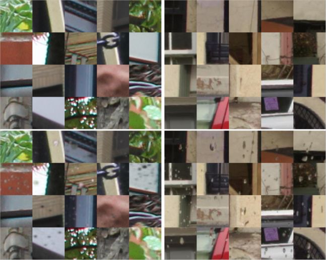
(see Fig. 4 for samples). Because the input and output ker- each xp using a fully-connected multilayer network f . We
nel sizes of our network differ, the network F produces a then form the predicted image y = depatchify({yp }) by
56 × 56 pixel prediction yi , which is compared against the taking the average of the patch predictions at pixels where
middle 56 × 56 pixels of the true clean subimage yi∗ . they overlap. In this context, the convolutional network F
We minimize the loss using Stochastic Gradient Descent can be expressed in terms of the patch-level network f as
(SGD). The update for a single step at time t is F (x) = depatchify({f (xp ) : xp ∈ patchify(x)}).
∂ In contrast to [2], our method trains the full network F ,
θt+1 ← θt − ηt (F (xi ) − yi∗ )T F (xi ) including patchification and depatchification. This drives
∂θ
a decorrelation of the individual predictions, which helps
where ηt is the learning rate hyper-parameter and i is a ran- both to remove occluders as well as reduce blur in the fi-
domly drawn index from the training set. The gradient is nal output. To see this, consider two adjacent patches y1
further backpropagated through the network F . and y2 with overlap regions yo1 and yo2 , and desired output
We initialize the weights at all layers by randomly draw- yo∗ . If we were to train according to the individual predic-
ing from a normal distribution with mean 0 and standard de- tions, the loss would minimize (yo1 − yo∗ )2 + (yo2 − yo∗ )2 ,
viation 0.001. The biases are initialized to 0. The learning the sum of their error. However, if we minimize the er-
2
rate is 0.001 with decay, so that ηt = 0.001/(1 + 5t · 10−7 ). ror of their average, the loss becomes yo1 +y 2
o2
− yo∗ =
1 ∗ 2 ∗ 2 ∗ ∗
We use no momentum or weight regularization. 4 [(yo1 − yo ) + (yo2 − yo ) + 2(yo1 − yo )(yo2 − yo )].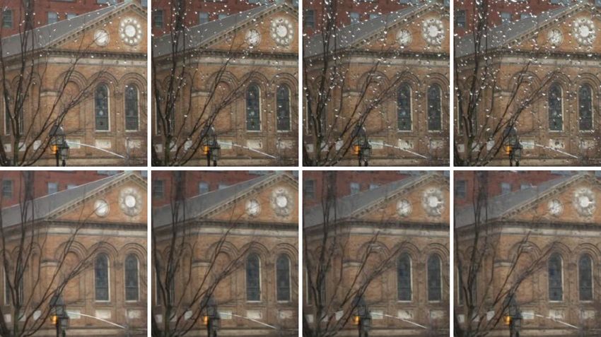
The new mixed term pushes the individual patch errors in
opposing directions, encouraging them to decorrelate.
   Fig. 3 depicts this for a real example. When trained at the
patch level, as in the system described by [2], each predic-
tion leaves the same residual trace of the noise, which their
average then maintains (b). When trained with our convolu-
tional network, however, the predictions decorrelate where
not perfect, and average to a better output (c).

2.4. Test-Time Evaluation
    By restricting the middle layer kernels to have 1 × 1 spa-
tial support, our method requires no synchronization un-
til the final summation in the last layer convolution. This
makes our method natural to parallelize, and it can eas-
ily be run in sections on large input images by adding
the outputs from each section into a single image output
buffer. Our Matlab GPU implementation is able to restore a                         Figure 4. Examples of clean (top row) and corrupted (bottom row)
3888 × 2592 color image in 60s using a nVidia GTX 580,                             patches used for training. The dirt (left column) was added syn-
                                                                                   thetically, while the rain (right column) was obtained from real
and a 1280 × 720 color image in 7s.
                                                                                   image pairs.

3. Training Data Collection
                                                                                   glass pane placed in front of the camera. We then solved
   The network has 753,664 weights and 1,216 biases                                a linear least-squares system for α and αD at each pixel;
which need to be set during training. This requires a large                        further details are included in the supplementary material.
number of training patches to avoid over-fitting. We now
describe the procedures used to gather the corrupted/clean                         3.2. Water Droplets
patch pairs2 used to train each of the dirt and rain models.                           Unlike the dirt, water droplets refract light around them
                                                                                   and are not well described by a simple additive model. We
3.1. Dirt                                                                          considered using the more sophisticated rendering model
   To train our network to remove dirt noise, we gener-                            of [8], but accurately simulating outdoor illumination made
ated clean/noisy image pairs by synthesizing dirt on im-                           this inviable. Thus, instead of synthesizing the effects of
ages. Similarly to [9], we also found that dirt noise was                          water, we built a training set by taking photographs of mul-
well-modeled by an opacity mask and additive component,                            tiple scenes with and without the corruption present. For
which we extract from real dirt-on-glass panes in a lab                            corrupt images, we simulated the effect of rain on a window
setup. Once we have the masks, we generate noisy images                            by spraying water on a pane of anti-reflective MgF2 -coated
according to                                                                       glass, taking care to produce drops that closely resemble
                  I 0 = pαD + (1 − α)I                                             real rain. To limit motion differences between clean and
                                                                                   rainy shots, all scenes contained only static objects. Further
Here, I and I 0 are the original clean and generated noisy                         details are provided in the supplementary material.
image, respectively. α is a transparency mask the same size
as the image, and D is the additive component of the dirt,                         4. Baseline Methods
also the same size as the image. p is a random perturbation
                                                                                       We compare our convolutional network against a non-
vector in RGB space, and the factors pαD are multiplied
                                                                                   convolutional patch-level network similar to [2], as well as
together element-wise. p is drawn from a uniform distri-
                                                                                   three baseline approaches: median filtering, bilateral fil-
bution over (0.9, 1.1) for each of red, green and blue, then
                                                                                   tering [18, 15], and BM3D [3]. In each case, we tuned
multiplied by another random number between 0 and 1 to
                                                                                   the algorithm parameters to yield the best qualitative per-
vary brightness. These random perturbations are necessary
                                                                                   formance in terms of visibly reducing noise while keeping
to capture natural variation in the corruption and make the
                                                                                   clean parts of the image intact. On the dirt images, we used
network robust to these changes.
                                                                                   an 8 × 8 window for the median filter, parameters σs = 3
   To find α and αD, we took pictures of several slide-
                                                                                   and σr = 0.3 for the bilateral filter, and σ = 0.15 for
projected backgrounds, both with and without a dirt-on-
                                                                                   BM3D. For the rain images, we used similar parameters,
   2 The corrupt patches still have many unaffected pixels, thus even with-        but adjusted for the fact that the images were downsampled
out clean/clean patch pairs in the training set, the network will still learn to   by half: 5 × 5 for the median filter, σs = 2 and σr = 0.3
preserve clean input regions.
                                                                                   for the bilateral filter, and σ = 0.15 for BM3D.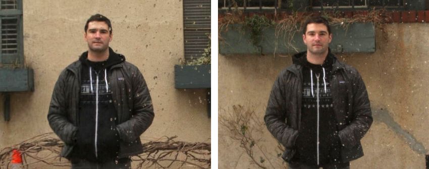
Original                                                            Our Output

Original                            Ours                            Nonconv                             Median

Figure 5. Example image containing dirt, and the restoration produced by our network. Note the detail preserved in high-frequency areas
like the branches. The nonconvolutional network leaves behind much of the noise, while the median filter causes substantial blurring.

                                                                        PSNR       Input     Ours Nonconv Median Bilateral BM3D
5. Experiments
                                                                        Mean       28.93 35.43        34.52    31.47     29.97     29.99
5.1. Dirt                                                              Std.Dev. 0.93         1.24      1.04     1.45      1.18      0.96
    We tested dirt removal by running our network on pic-                Gain         -      6.50      5.59     2.53      1.04      1.06
tures of various scenes taken behind dirt-on-glass panes.             Table 1. PSNR for our convolutional neural network, nonconvolu-
Both the scenes and glass panes were not present in the               tional patch-based network, and baselines on a synthetically gen-
training set, ensuring that the network did not simply mem-           erated test set of 16 images (8 scenes with 2 different dirt masks).
orize and match exact patterns. We tested restoration of              Our approach significantly outperforms the other methods.
both real and synthetic corruption. Although the training             than the three baselines, which do not make use of the struc-
set was composed entirely of synthetic dirt, it was represen-         ture in the corruption that the networks learn.
tative enough for the network to perform well in both cases.             We also applied our network to two types of artificial
    The network was trained using 5.8 million examples                noise absent from the training set: synthetic “snow” made
of 64 × 64 image patches with synthetic dirt, paired with             from small white line segments, and “scratches” of random
ground truth clean patches. We trained only on examples               cubic splines. An example region is shown in Fig. 6. In
where the variance of the clean 64 × 64 patch was at least            contrast to the gain of +6.50 dB for dirt, the network leaves
0.001, and also required that at least 1 pixel in the patch           these corruptions largely intact, producing near-zero PSNR
had a dirt α-mask value of at least 0.03. To compare to [2],          gains of -0.10 and +0.30 dB, respectively, over the same
we trained a non-convolutional patch-based network with               set of images. This demonstrates that the network learns to
patch sizes corresponding to our convolution kernel sizes,            remove dirt specifically.
using 20 million 16 × 16 patches.
                                                                      5.1.2 Dirt Results
5.1.1      Synthetic Dirt Results                                     Fig. 5 shows a real test image along with our output and the
We first measure quantitative performance using synthetic             output of the patch-based network and median filter. Be-
dirt. The results are shown in Table 1. Here, we generated            cause of illumination changes and movement in the scenes,
test examples using images and dirt masks held out from the           we were not able to capture ground truth images for quanti-
training set, using the process described in Section 3.1. Our         tative evaluation. Our method is able to remove most of the
convolutional network substantially outperforms its patch-            corruption while retaining details in the image, particularly
based counterpart. Both neural networks are much better               around the branches and shutters. The non-convolutional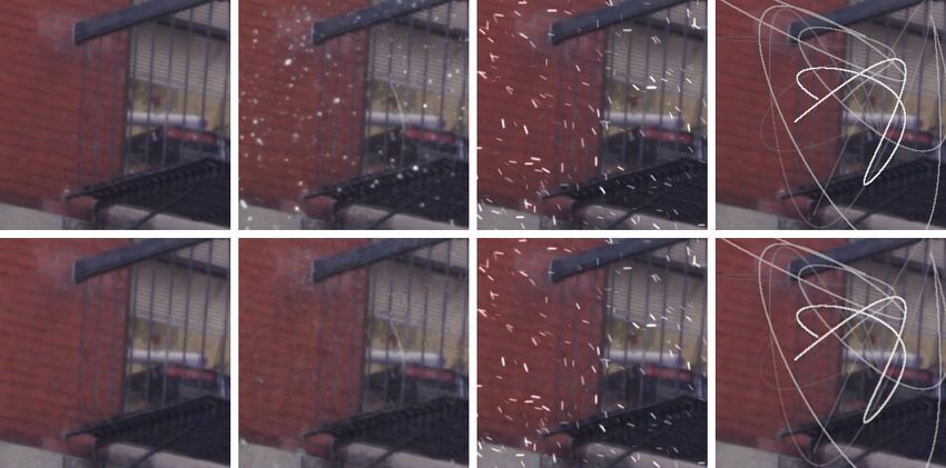
(a) (b) (c) (d)
Figure 6. Our dirt-removal network applied to an image with (a) Figure 8. Shot from the rain video sequence (see supplementary
no corruption, (b) synthetic dirt, (c) artificial “snow” and (d) ran- video), along with the output of our network. Note each frame is
dom “scratches.” Because the network was trained to remove dirt, processed independently, without using any temporal information
it successfully restores (b) while leaving the corruptions in (c,d) or background subtraction.
largely untouched. Top: Original images. Bottom: Output.
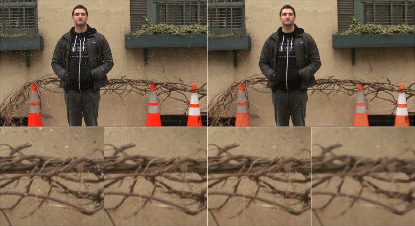
As before, our network is able to remove most of the
network leaves many pieces of dirt behind, while the me- water droplets, while preserving finer details and edges rea-
dian filter loses much detail present in the original. Note sonably well. The non-convolutional network leaves behind
also that the neural networks leave already-clean parts of additional droplets, e.g. by the subject’s face in the top im-
the image mostly untouched. age; it performs somewhat better in the bottom image, but
Two common causes of failure of our model are large blurs the subject’s hand. The median filter must blur the
corruption, and very oddly-shaped or unusually colored cor- image substantially before visibly reducing the corruption.
ruption. Our 16 × 16 input kernel support limits the size of However, the neural networks mistake the boltheads on the
corruption recognizable by the system, leading to the for- bench for raindrops, and remove them.
mer. The latter is caused by a lack of generalization: al- Despite the fact that our network was trained on static
though we trained the network to be robust to shape and scenes to limit object motion between clean/noisy pairs, it
color by supplying it a range of variations, it will not recog- still preserves animate parts of the images well: The face
nize cases too far from those seen in training. Another in- and body of the subject are reproduced with few visible ar-
teresting failure of our method appears in the bright orange tifacts, as are grass, leaves and branches (which move from
cones in Fig. 5, which our method reduces in intensity — wind). Thus the network can be applied to many scenes
this is due to the fact that the training dataset did not contain substantially different from those seen in training.
any examples of such fluorescent objects. More examples
5.2.2 Real Rain Results
are provided in the supplementary material.
A picture taken using actual rain is shown in Fig. 8. We
5.2. Rain include more pictures of this time series as well as a video
We ran the rain removal network on two sets of test data: in the supplementary material. Each frame of the video was
(i) pictures of scenes taken through a pane of glass on which presented to our algorithm independently; no temporal fil-
we sprayed water to simulate rain, and (ii) pictures of scenes tering was used. To capture the sequence, we set a clean
taken while it was actually raining, from behind an initially glass pane on a tripod and allowed rain to fall onto it, tak-
clean glass pane. Both sets were composed of real-world ing pictures at 20s intervals. The camera was placed 0.5m
outdoor scenes not in the training set. behind the glass, and was focused on the scene behind.
We trained the network using 6.5 million examples of Even though our network was trained using sprayed-on
64 × 64 image patch pairs, captured as described in Sec- water, it was still able to remove much of the actual rain.
tion 3.2. Similarly to the dirt case, we used a variance The largest failures appear towards the end of the sequence,
threshold of 0.001 on the clean images and required each when the rain on the glass is very heavy and starts to ag-
training pair to have at least 1 pixel difference over 0.1. glomerate, forming droplets larger than our network can
handle. Although this is a limitation of the current ap-
5.2.1 Water Droplets Results proach, we hope to address such cases in future work.
Examples of our network removing sprayed-on water is Lastly, in addition to pictures captured with a DSLR, in
shown in Fig. 7. As was the case for the dirt images, we Fig. 9 we apply our network to a picture taken using a smart-
were not able to capture accurate ground truth due to illu- phone on a train. While the scene and reflections are pre-
mination changes and subject motion. Since we also do not served, raindrops on the window are removed, though a few
have synthetic water examples, we analyze our method in small artifacts do remain. This demonstrates that our model
this mode only qualitatively. is able to restore images taken by a variety of camera types.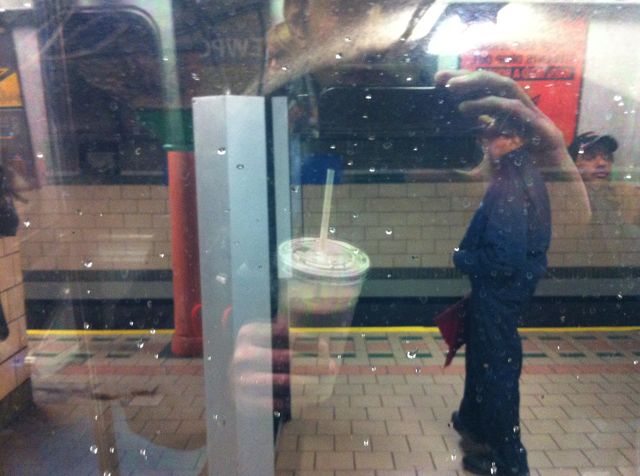
Original                                                              Our Output

Original                           Ours                               Nonconv                            Median

Original                                                              Our Output

Original                           Ours                               Nonconv                            Median

Figure 7. Our network removes most of the water while retaining image details; the non-convolutional network leaves more droplets
behind, particularly in the top image, and blurs the subject’s fingers in the bottom image. The median filter blurs many details, but still
cannot remove much of the noise.
6. Summary
    We have introduced a method for removing rain or dirt
artifacts from a single image. Although the problem appears
underconstrained, the artifacts have a distinctive appearance
which we are able to learn with a specialized convolutional
network and a carefully constructed training set. Results on
real test examples show most artifacts being removed with-
out undue loss of detail, unlike existing approaches such as
median or bilateral filtering. Using a convolutional network
accounts for the error in the final image prediction, provid-
ing a significant performance gain over the corresponding
patch-based network.
    The quality of the results does however depend on the
statistics of test cases being similar to those of the training
set. In cases where this does not hold, we see significant
artifacts in the output. This can be alleviated by expanding
the diversity and size of the training set. A second issue is
that the corruption cannot be much larger than the training
patches. This means the input image may need to be down-
sampled, e.g. as in the rain application, leading to a loss of
resolution relative to the original.
    Although we have only considered day-time outdoor
shots, the approach could be extended to other settings such
as indoor or night-time, given suitable training data. It could
also be extended to other problem domains such as scratch                           Figure 9. Top: Smartphone shot through a rainy window on a train.
removal or color shift correction.                                                  Bottom: Output of our algorithm.
    Our algorithm provides the underlying technology for a
                                                                                     [8] J. Gu, R. Ramamoorthi, P. Belhumeur, and S. Nayar. Dirty Glass: Rendering
number of potential applications such as a digital car wind-                             Contamination on Transparent Surfaces. In Eurographics, Jun 2007. 4
shield to aid driving in adverse weather conditions, or en-                          [9] J. Gu, R. Ramamoorthi, P. Belhumeur, and S. Nayar. Removing Image Artifacts
                                                                                         Due to Dirty Camera Lenses and Thin Occluders. SIGGRAPH Asia, Dec 2009.
hancement of footage from security or automotive cam-                                    2, 4
eras in exposed locations. These would require real-time                            [10] V. Jain and S. Seung. Natural image denoising with convolutional networks. In
                                                                                         NIPS, 2008. 2
performance not obtained by our current implementation.                             [11] J. Jancsary, S. Nowozin, and C. Rother. Loss-specific training of non-parametric
High-performance low-power neural network implementa-                                    image restoration models: A new state of the art. In ECCV, 2012. 2
tions such as the NeuFlow FPGA/ASIC [6] would make                                  [12] Y. LeCun, L. Bottou, Y. Bengio, and P. Haffner. Gradient-based learning ap-
                                                                                         plied to document recognition. Proc. IEEE, 86(11):2278–2324, Nov 1998. 2
real-time embedded applications of our system feasible.                             [13] A. Levin and B. Nadler. Natural image denoising: Optimality and inherent
                                                                                         bounds. In CVPR, 2011. 1
Acknowledgements                                                                    [14] B. A. Olshausen and D. J. Field. Sparse coding with an overcomplete basis set:
   The authors would like to thank Ross Fadeley and Dan                                  A strategy employed by V1? Vision Research, 37(23):3311–3325, 1997. 2
                                                                                    [15] S. Paris and F. Durand. A fast approximation of the bilateral filter using a signal
Foreman-Mackay for their help modeling, as well as David                                 processing approach. In ECCV, pages IV: 568–580, 2006. 4
W. Hogg and Yann LeCun for their insight and suggestions.                           [16] J. Portilla, V. Strela, M. J. Wainwright, and E. P. Simoncelli. Image denoising
                                                                                         using scale mixtures of Gaussians in the wavelet domain. IEEE Trans Image
Financial support for this project was provided by Microsoft                             Processing, 12(11):1338–1351, November 2003. 2
Research and NSF IIS 1124794 & IIS 1116923.                                         [17] M. Roser and A. Geiger. Video-based raindrop detection for improved image
                                                                                         registration. In ICCV Workshop on Video-Oriented Object and Event Classifi-
References                                                                               cation, Kyoto, Japan, September 2009. 2
                                                                                    [18] C. Tomasi and R. Manduchi. Bilateral filtering for gray and color images. In
[1] P. Barnum, S. Narasimhan, and K. Takeo. Analysis of rain and snow in fre-            CVPR, 1998. 4
    quency space. IJCV, 86(2):256–274, 2010. 2                                      [19] R. G. Willson, M. W. Maimone, A. E. Johnson, and L. M. Scherr. An optical
[2] H. Burger, C. Schuler, and S. Harmeling. Image denoising: Can plain neural           model for image artifacts produced by dust particles on lenses. In i-SAIRAS,
    networks compete with BM3D? In CVPR, 2012. 2, 3, 4, 5                                volume 1, 2005. 2
[3] K. Dabov, A. Foi, V. Katkovnik, and K. Egiazarian. Image denoising with         [20] J. Xie, L. Xu, and E. Chen. Image denoising and inpainting with deep neural
    block-matching and 3D filtering. In Proc. SPIE Electronic Imaging, 2006. 1, 4        networks. In NIPS, 2012. 2
[4] B. Dong, H. Ji, J. Li, Z. Shen, and Y. Xu. Wavelet frame based blind image      [21] S. Zhang and E. Salari. Image denosing using a neural network based non-linear
    inpainting. Applied and Comp’l Harmonic Analysis, 32(2):268–279, 2011. 2             filter in the wavelet domain. In ICASSP, 2005. 2
[5] M. Elad and M. Aharon. Image denoising via learned dictionaries and sparse      [22] C. Zhou and S. Lin. Removal of image artifacts due to sensor dust. In CVPR,
    representation. In CVPR, 2006. 2                                                     2007. 2
[6] C. Farabet, B. Martini, B. Corda, P. Akselrod, E. Culurciello, and Y. LeCun.    [23] S. C. Zhu and D. Mumford. Prior learning and gibbs reaction-diffusion. PAMI,
    NeuFlow: A runtime reconfigurable dataflow processor for vision. In IEEE             19(11):1236–1250, 1997. 2
    Workshop on Embedded Computer Vision (ECV at CVPR), 2011. 8                     [24] D. Zoran and Y. Weiss. From learning models of natural image patches to whole
[7] K. Garg and S. Nayar. Detection and removal of rain from videos. In CVPR,            image restoration. In ICCV, 2011. 2
    pages 528–535, 2004. 2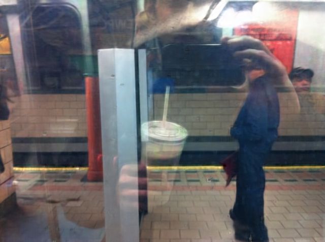
You can also read