Single-Shot 3D Shape Reconstruction Using Structured Light and Deep Convolutional Neural Networks - MDPI
←
→
Page content transcription
If your browser does not render page correctly, please read the page content below
sensors
Article
Single-Shot 3D Shape Reconstruction Using
Structured Light and Deep Convolutional
Neural Networks
Hieu Nguyen 1,2 , Yuzeng Wang 3 and Zhaoyang Wang 1, *
 1    Department of Mechanical Engineering, The Catholic University of America, Washington, DC 20064, USA
 2    Neuroimaging Research Branch, National Institute on Drug Abuse, National Institutes of Health,
      Baltimore, MD 21224, USA; hieu.nguyen@nih.gov
 3    School of Mechanical Engineering, Jinan University, Jinan 250022, China; me_wangyz@ujn.edu.cn
 *    Correspondence: wangz@cua.edu; Tel.: +1-202-319-6175

 Received: 4 June 2020; Accepted: 30 June 2020; Published: 3 July 2020

 Abstract: Single-shot 3D imaging and shape reconstruction has seen a surge of interest due to
 the ever-increasing evolution in sensing technologies. In this paper, a robust single-shot 3D shape
 reconstruction technique integrating the structured light technique with the deep convolutional neural
 networks (CNNs) is proposed. The input of the technique is a single fringe-pattern image, and the
 output is the corresponding depth map for 3D shape reconstruction. The essential training and
 validation datasets with high-quality 3D ground-truth labels are prepared by using a multi-frequency
 fringe projection profilometry technique. Unlike the conventional 3D shape reconstruction methods
 which involve complex algorithms and intensive computation to determine phase distributions
 or pixel disparities as well as depth map, the proposed approach uses an end-to-end network
 architecture to directly carry out the transformation of a 2D image to its corresponding 3D depth map
 without extra processing. In the approach, three CNN-based models are adopted for comparison.
 Furthermore, an accurate structured-light-based 3D imaging dataset used in this paper is made
 publicly available. Experiments have been conducted to demonstrate the validity and robustness
 of the proposed technique. It is capable of satisfying various 3D shape reconstruction demands in
 scientific research and engineering applications.

 Keywords: three-dimensional image acquisition; three-dimensional sensing; three-dimensional
 shape reconstruction; depth measurement; structured light; fringe projection; convolutional neural
 networks; deep machine learning

1. Introduction
      Non-contact 3D shape reconstruction using the structured-light techniques is commonly used
in a broad range of applications including machine vision, reverse engineering, quality assurance,
3D printing, entertainment, etc. [1–11]. The technique typically retrieves the depth or height
information with an algorithm based on geometric triangulation, where the structured light helps
facilitate the required image matching or decoding process. According to the number of images
required for each 3D reconstruction, the structured-light techniques can be classified into two categories:
multi-shot [12–15] and single-shot [16–18]. The multi-shot techniques are capable of capturing
high-resolution 3D images at a limited speed and are thus widely used as industrial metrology for
accurate shape reconstructions. By contrast, the single-shot techniques can acquire 3D images at
a fast speed to deal with dynamic scenes and are receiving tremendous attention in the fields of
entertainment and robotics. As technologies evolve at an ever-increasing pace, applying the concept

Sensors 2020, 20, 3718; doi:10.3390/s20133718                                 www.mdpi.com/journal/sensors
Sensors 2020, 20, 3718                                                                           2 of 13

of deep machine learning to the highly demanded single-shot 3D shape reconstructions has now
become feasible.
      In the machine learning field, deep convolutional neural networks (CNNs) have found numerous
applications in object detection, image classification, scene understanding, medical image analysis,
and natural language processing, etc. The recent advances of using the deep CNNs for image
segmentation intend to make the network architecture an end-to-end learning process. For example,
Long et al. [19] restored the downsampled feature map to the original size of the input using
backwards convolution. An impressive network architecture, named UNet and proposed by
Ronneberger et al. [20], extended the decoding path from Long’s framework to yield a precise output
with a relatively small number of training images. Similarly, Badrinarayanan et al. [21] used an idea
of upsampling the lowest of the encoder output to improve the resolution of the output with less
computational resources.
      In the CNN-based 3D reconstruction and depth detection applications, Eigen et al. [22] and
Liu et al. [23] respectively proposed a scheme to conduct the depth estimation from a single view
using the CNNs. In their work, they used a third-party training dataset produced by Kinect RGB-D
sensors, which has low accuracy and is insufficient for good learning. Inspired by these two methods,
Choy et al. [24] proposed a novel architecture which employs recurrent neural networks (RNNs) among
the autoencoder CNNs for single- and multi-view 3D reconstructions. Later, Duo et al. [25] proposed a
deep CNN scheme to reconstruct the 3D face shape from a single facial image. Although Duo’s
framework showed outstanding performance with a synthetic and publicly available database,
it requires a post-processing step which further relies on combining a set of shape and blend-shape
basis. Recently, Paschalidou et al. [26] proposed an end-to-end Raynet to reconstruct dense 3D models
from multiple images by combining the CNNs with a Markov random field. A common issue with
these existing techniques is the lack of using high-accuracy training data.
      Over the past year, the utilizing of the CNN frameworks for fringe analysis has become active
in the optics field. For instance, Feng et al. [27,28] integrated the deep CNNs with the phase-shifting
scheme for unwrapped phase detections. Yin et al. [29] removed the phase ambiguities in the phase
unwrapping process with two groups of phase-shifted fringe patterns and deep learning. Jeught [30]
proposed a neural network with a large simulated training dataset to acquire the height information
from a single fringe pattern. A number of other investigations [31–35] have also shown promising
results on using the CNN models to improve the estimation and determination of phase distributions.
In addition, various techniques have been proposed to reduce the noise in fringe pattern analysis using
deep learning schemes [36–38].
      Based on the successful applications of the CNNs to image segmentation, 3D scene reconstruction,
and fringe pattern analysis, the exploration of utilizing the deep CNNs to accurately reconstruct the
3D shapes from a single structured-light image should be quite viable. With numerous parameters,
a deep CNN model can be trained to approximate a very complex non-linear regressor that is capable
of mapping a conventional structured-light image to its corresponding 3D depth or height map.
At present, the robustness and importance of integrating the deep CNNs with one of the most
widely used structured-light methods, fringe projection profilometry (FPP) technique, have started
drawing lots of attention and are emerging quickly. In this paper, such integration for accurate
3D shape reconstruction is investigated in a different perspective. The main idea is to transform a
single-shot image, which has a high-frequency fringe pattern projected on the target, into a 3D image
using a deep CNN that has a contracting encoder path and an expansive decoder path. Compared
with the conventional 3D shape measurement techniques, the proposed technique is considerably
simpler without using any geometric information or any complicated registration and triangulation
computation. A schematic of the single-shot FPP-based 3D system is shown in Figure 1.
Sensors 2020, 20, 3718 3 of 13
ܻ௪ ܚܗܜ܋܍ܒܗܚ۾
ܺ௪
ܼ௪
۱܉ܚ܍ܕ܉
Figure 1. Schematic of the FPP-based 3D imaging and shape measurement system.
Using real and accurate training data is essential for a reliable machine learning model. Because the
FPP technique is one of the most accurate 3D shape measurement techniques and is able to perform
3D imaging with accuracy better than 0.1 mm, it is employed in this work to generate the required
datasets for learning and evaluation. That is, the system shown in Figure 1 serves two purposes: it
first provides the conventional FPP technique with multi-shot images (e.g., 16 images in each entry) to
prepare the ground-truth data for the training and validation of the networks; then acquires single-shot
images (i.e., one image in each entry) for the application of the proposed technique.
The rest of the paper is elaborated as follows. Section 2.1 reviews the FPP-based technique to
generate high-accuracy training datasets. Section 2.2 describes the details of the proposed network
architectures. Section 3 provides a few experimental results. Finally, Sections 4 and 5 conclude the
paper with discussions and a brief summary.
2. Methodology
2.1. Fringe Projection Profilometry (FPP) Technique for Training Data Generation
The most reliable FPP technique involves projecting a set of phase-shifted sinusoidal fringe
patterns from a projector onto the objects, where the surface depth or height information is naturally
encoded into the camera-captured fringe patterns for the subsequent 3D reconstruction process.
Technically, the fringe patterns help establish the correspondences between the captured image and the
original reference image projected by the projector. In practice, the technique reconstructs the 3D shapes
through determining the height or depth map from the phase distributions of the captured fringe
patterns. The phase extraction process normally uses phase-shifted fringe patterns to calculate the
fringe phase. In general, the original fringes are straight, evenly spaced, and vertically (or horizontally)
oriented. They are numerically generated with the following function [39–42]:
( p) ( p)
h u i
Ij (u, v) = I0 1 + cos(φ + δj ) = I0 1 + cos(2π f + δj ) (1)
W
where I ( p) is the intensity value of the pattern at pixel coordinate (u, v); the subscript j denotes the jth
phase-shifted image with j = {1, 2, ..., m}, and m is the number of the phase-shift steps (e.g., m = 4);
( p)
I0 is a constant coefficient indicating the value of intensity modulation; f is the number of fringes
in the pattern; W is the width of the generated image; δ is the phase-shift amount; and φ is the
fringe phase.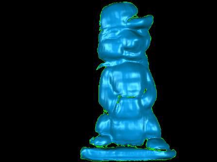
Sensors 2020, 20, 3718 4 of 13
The projector projects the fringe patterns onto the target of interest, and the camera captures the
images of the target with projected fringes. The phase distribution in the images can be calculated by
using a standard phase-shifting algorithm, typically the four-step one. The phase φ at a pixel (u, v) can
be determined as:
I (u, v) − I2 (u, v)
φw (u, v) = arctan 4 , (2)
I1 (u, v) − I3 (u, v)
In the equation, I (u, v) indicates the intensity value at the pixel coordinate (u, v) in the captured
images, and the subscript numbers 1–4 represents the sequential steps of the four phase-shifted
patterns in the images.
It can be seen from the equation that the phase value is wrapped in a range of 0 to 2π (denoted
with a superscript w) and must be unwrapped to obtain the true phase. In order to cope with the
phase-unwrapping difficulty encountered in the cases of complex shapes and geometric discontinuities,
a scheme of using multi-frequency fringe patterns is often employed in practice. The corresponding
unwrapped phase distributions can be calculated from [43–45]:
fi
φi−1 f − φiw
φi (u, v) = φiw (u, v) + INT i −1 2π (3)
2π
where φ is the unwrapped phase; i indicates the ith fringe-frequency pattern with i = {2, 3, ..., n}, and n
is the number of fringe frequencies; INT represents the function of rounding to the nearest integer; f i
is the number of fringes in the ith projection pattern, with f n > f n−1 > ... > f 1 = 1; and φ1 = φ1w is
f
satisfied for f 1 = 1. The ratio between two adjacent fringe frequencies f i is normally smaller or equal
i −1
to 5 to reduce the noise effect and ensure the reliability of the algorithm. A practical example is n = 4
with f 4 = 100, f 3 = 20, f 2 = 4, and f 1 = 1. It can be seen that four images for each frequency and four
frequencies for each measurement indicate a total of 16 images for each accurate FPP measurement.
The essential task of the FPP technique is to retrieve the depth or height map from the calculated
phase distributions of the highest frequency fringes with the highest possible accuracy. The governing
equation for a generalized setup where the system components can be arbitrarily positioned [46,47] is:
Cp|
zw =
Dp|
C = {1 c1 c2 c3 · · · c17 c18 c19 }
(4)
D = {d0 d1 d2 d3 · · · c17 d18 d19 }
n o
p = 1 φ u uφ v vφ u2 u2 φ uv uvφ v2 v2 φ u3 u3 φ u2 v u2 vφ uv2 uv2 φ v3 v3 φ
where zw is the height or depth at the point corresponding to the pixel (u, v) in the captured images,
and it is also the z-coordinate of the point in the reference or world coordinate system; φ is the
unwrapped phase of the highest-frequency fringe pattern at the same pixel; and c1 − c19 and d0 − d19 are
constant coefficients associated with geometrical and other system parameters. The 39 coefficients can
be determined by a calibration process using a few gage objects that have many points with zw precisely
known. After the height or depth map is obtained using Equation (4), the other two coordinates xw
and yw can be easily determined upon knowing the camera and lens parameters. For this reason,
the two terms, depth measurement and 3D shape reconstruction, can be often used interchangeably.
The FPP technique is employed to generate the training datasets, including the validation data.
Once the training datasets are available, they can be directly fed into deep CNN models for subsequent
learning process. It is noteworthy that the FPP technique is also used to provides the ground-truth
results of the test dataset for evaluation purpose.
Sensors 2020, 20, 3718                                                                                   5 of 13

2.2. Network Architecture
     Given a single-shot input image of an object or a few objects, the proposed approach uses a deep
neural network to transform the image into a 3D point cloud from the fringe patterns presented
in the image. Figure 2 illustrates how the proposed integration of fringe projection with deep
machine learning works. The adopted network is mainly made up of two components: the encoder
path and the decoder path. The encoder path includes convolution and pooling operations that
are capable of detecting essential features from the input image. The decoder path, on the other
hand, contains transpose convolution and unpooling operations that can stack and concatenate lower
resolution feature maps to form higher resolution layers. The output of the network is a 3D depth or
height map corresponding to the input image.

                                                Convolution + ReLU
                                                Max Pooling
                                                Upsampling
                                                Convolution 1x1

          Figure 2. Illustration of the single-shot 3D shape reconstruction system using FPP and CNNs.

     Three different deep CNNs are adopted in this work for comparison to find the best approach.
The three networks are as follows:

•     Fully convolutional networks (FCN). The FCN is a well-known network for semantic
      segmentation. FCN adopts the encoder path from the contemporary classification networks
      and transforms the fully connected layers into convolution layers before upsampling the coarse
      output map to the same size as the input. The FCN-8s architecture [19] is adopted in this paper
      to prevent the loss of spatial information, and the network has been modified to work with the
      input image and yield the desired output information of depth.
•     Autoencoder networks (AEN). The AEN has an encoder path and a symmetric decoder path.
      The proposed AEN has totally 33 layers, including 22 standard convolution layers, 5 max pooling
      layers, 5 transpose operation layers, and a 1 × 1 convolution layer.
•     UNet. The UNet is also a well-known network [20], and it has a similar architecture to the
      AEN. The key difference is that in the UNet the local context information from the encoder
      path is concatenated with the upsampled output, which can help increase the resolution of the
      final output.

      The architectures of the three deep CNNs are shown in Figure 3.
      In the learning process of the three CNNs, the training or validation dataset in each CNN model
is a four-dimensional array of size s × h × w × c, where s is the number of the data samples; h and w
are the spatial dimensions or image dimensions; c is the channel dimension, with c = 1 for grayscale
images and c = 3 for color images. The networks contain convolution, pooling, transpose convolution,
and unpooling layers; they do not contain any fully connected layers. Each convolution layer learns the
local features from the input and produces the output features where the spatial axes of the output map
remain the same but the depth axis changes following the convolution operation filters. A nonlinear
activation function named rectified linear unit (ReLU), expressed as max (0, x ), is employed in each
convolution layer.
      In the chain-based architecture, each layer in the network is given by [48]

                                               h = g( W| x + b )                                            (5)
Sensors 2020, 20, 3718 6 of 13
where h is the output vector; function g is called an activation function; x is a vector of input;
the parameters W in a matrix form and b in a vector form are optimized by the learning process.
ሺሻ
1024
512
1024
512
512
512
256
256
256
128
128
256
128
256
256
64
128
128
128
32
64
64
1
32
32
32
ሺሻ
512
1024
1024
512
512
512
512
256
512
256
256
256
256
128
256
64
128
128
128
128
128
32
64
64
64
64
64
1
32
32
32
32
32
ܥ
ܥ
ܥ
ܥ ܥ
ሺ ሻ
1024
1024
512
512
256
512
512
512
512
512
256
256
128
256
256
256
256
128
128
64
128
128
128
128
64
64
32
64
64
64
64
1
32
32
32
32
32
32
Convolution + ReLU
Max Pooling
Upsampling
Convolution 1x1
Summation
ܥConcatenation
Figure 3. The proposed network architectures: (a) Fully convolutional networks (FCN),
(b) Autoencoder networks (AEN), and (c) UNet.
The max pooling layers with a 2 × 2 window and a stride of 2 are applied to downsample the
feature maps through extracting only the max value in each window. In the AEN and UNet, the 2D
transpose convolution layers are applied in the decoder path to transform the lower feature input back
to a higher resolution. Finally, a 1 × 1 convolution layer is attached to the final layer to transform the
feature maps to the desired depth or height map. Unlike the conventional 3D shape reconstruction
schemes that often require complex algorithms based on a profound understanding of techniques,
the proposed approach depends on numerous parameters in the networks, which are automatically
trained, to play a vital role in the single-shot 3D reconstruction.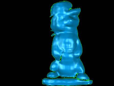
Sensors 2020, 20, 3718                                                                              7 of 13

3. Experiments and Results
     An experiment has been conducted to validate the proposed approach. The experiment uses
a desktop computer with an Intel Core i7-980 processor, a 16-GB RAM, and a Nvidia GeForce GTX
1070 graphics card as well as an Epson PowerLite98 projector and a Silicon Video 643M camera.
Keras, a popular Python deep learning library, is utilized in programming implementation. In addition,
Nvidia’s cuDNN deep neural network library is adopted to speed up the training process. The field
of view of the experiment is about 155 mm, and the distance from the camera to the scene of interest
is around 1.2 m. This working distance is typical in real applications of the 3D shape measurement,
and it can be substantially shorter or longer without affecting the nature of the proposed work. In the
experiments, a number of small plaster sculptures serve as the objects, whose sizes and surface natures
are suitable for producing reliable and accurate 3D datasets.

3.1. Training and Test Data Acquisition
      Unlike the synthetic data adopted by plenty of recent research, three different types of CNNs
have been tested using real collected training data. The experiment uses four fringe frequencies
(1, 4, 20, and 100) and the four-step phase-shifting schemes, which usually yield a good balance
among accuracy, reliability, and capability. The first image of the last frequency (i.e., f 4 = 100) is
chosen as the input image, and all other 15 images are captured solely for the purpose of creating
the ground-truth 3D height labels. Totally, the experiment generated 1120, 140, and 140 samples
in the training, validation, and test datasets, respectively; and each sample contains a single fringe
image of the object(s) and a corresponding height map. The data split ratio is 80%–10%–10% and
is appropriate for such a case of small datasets. The datasets have been made publicly available for
download (Ref. [49]). Supplementary Video S1 shows the input images and the ground-truth labels of
the training and test data side by side. It is noted that the background is neither mandatory nor has to
be flat, and it is shown in the input images but hidden in the visualization for better demonstration
purposes. Moreover, the original shadow areas are excluded from the learning process.

3.2. Training, Analysis, and Evaluation
      The training and validation data are applied to the learning process of the FCN, AEN,
and UNet models. The optimization Adam [50] adopts a total of 300 epochs with a mini-batch
size of 2 images. The learning rate is reduced by half whenever the validation loss does not
improve within 20 consecutive epochs. A few regularization schemes, including data augmentation,
weight regularization, data shuffling, and dropout, are employed to tackle the over-fitting problem.
Furthermore, the grid search method is conducted to obtain the best hyperparameters for the training
model. In order to check the network performance as the training process iterates, a callback is
performed at the end of each epoch on a randomly pre-selected test image to predict the 3D shapes
using the updated model parameters (see Supplementary Video S2). The learning can adopt either the
binary cross-entropy or the mean squared error as the loss function. If the loss function is set as binary
cross-entropy, the ground truth data is scaled back to the value range between 0 and 1.
      The evaluation is carried out by calculating the mean relative error (MRE) and the root mean
squared error (RMSE) of the reconstructed 3D shapes. Table 1 shows the performance errors of the
three CNN models for single-shot 3D shape reconstruction. It can be seen that the FCN model yields
the largest error among the three CNNs, and its learning time is also the longest because of the involved
element-wise summation. The AEN model requires the least learning time, but its performance is
slightly inferior to that of the UNet in terms of accuracy. It is noticed that the network generally
performs better when the models are trained through a smaller batch size.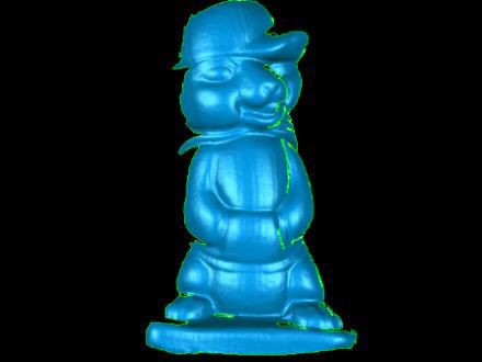
Sensors 2020, 20, 3718                                                                                      8 of 13

                                       Table 1. Performance evaluation of the CNNs.

                                    Model                 FCN            AEN             UNet
                              Training Time               7h              5h              6h
                                             MRE      1.28 ×   10−3   8.10 ×   10−4   7.01 × 10⁻⁴
                         Training
                                         RMSE (mm)        1.47           0.80            0.71
                                             MRE      1.78 ×   10−3   1.65 ×   10−3   1.47 × 10⁻³
                         Validation
                                         RMSE (mm)        1.73           1.43            1.27
                                             MRE       2.49×   10−3   2.32 ×   10−3   2.08 × 10⁻³
                            Test
                                         RMSE (mm)        2.03           1.85            1.62

     Figure 4 demonstrates a visual comparison of the ground-truth 3D data and the reconstructed 3D
data acquired with the three networks. The first image in each row is a representative input, and the
next is the corresponding 3D ground-truth image. The following three images in each row are the
reconstructed results from the FCN, AEN, and UNet models, respectively. Figure 5 shows the height
distributions relative to the background plane along an arbitrary line highlighted in each of the initial
input image. Again, it is evident from Figures 4 and 5 that the AEN and UNet models perform better
than the FCN model. The main reason is that the FCN abruptly restores the high-resolution feature
map from the lower one by using the bilinear upsampling operators, consequently many details are
lacking in the final reconstructed 3D results. The AEN and UNet each consists of its decoder path that
is symmetric to the encoder path, which helps steadily propagate the context information between
layers to produce features depicting detailed information. Unlike the AEN, the UNet contains the
concatenation operation to send extra local features to the decoder path. This handling helps the
network to perform the best among the three networks.

          7HVW,PDJH              *URXQG7UXWK          )&1                    $(1              81HW

                         Figure 4. 3D reconstruction results of two representative test images.

     Reconstructing the 3D shapes of multiple separated objects at different depths is a task that cannot
be fulfilled by typical single-shot fringe projection methods because of the fringe phase discontinuity
issue. Nevertheless, the surface discontinuity is not a problem for the proposed approaches since the
CNN models learn from datasets with labels directly and do not involve phase calculation. An example
of the 3D shape reconstruction of multiple separate objects using the UNet model is shown in Figure 6.
     A final experiment has been accomplished to demonstrate the performance comparison of the
proposed UNet technique with two existing popular techniques: the conventional FPP technique and
the 3D digital image correlation (3D-DIC) technique [51–53]. Technically, the 3D-DIC technique is
considered as a single-shot stereo vision method as it requires simultaneously capturing two images
from two different views with two cameras. The 3D-DIC technique relies on the area- or block-based
image registration, so it generally yields measurement resolution lower than that provided by the FPP
Sensors 2020, 20, 3718                                                                                                                                            9 of 13

technique. Figure 7 displays the visual comparison of the 3D shape reconstructions obtained from
three techniques. It is evident from the figure that the FPP technique gives the highest measurement
accuracy, and the proposed UNet technique is slightly inferior to the 3D-DIC technique in terms of
accuracy. It is noteworthy that the 3D reconstruction time for a new single image using the proposed
method is generally less than 50 ms on the aforementioned computer, which indicates that a real-time
3D shape reconstruction is practicable. In contrast, the typical running times of the FPP and the 3D-DIC
techniques are in the range of 0.1 to 2 s.

                                               FCN                                 (a)                                 FCN                                  (b)
                                   36          AEN                                                           36        AEN
                                               UNet                                                                    UNet

                                                                                         Height/Depth (mm)
               Height/Depth (mm)

                                   24          Ground truth                                                  24        Ground truth

                                   12                                                                        12

                                   0                                                                         0

                                   -12                                                                       -12
                                           0     100    200   300   400    500   600                               0     100    200   300   400    500     600
                                                         Image width (pixel)                                                     Image width (pixel)

      Figure 5. Height distributions: (a) along a line highlighted in the first test image in Figure 4, (b) along
      a line highlighted in the second test image in Figure 4.

                                         7HVW,PDJH                              *URXQG7UXWK                                                    81HW

                                                 Figure 6. 3D reconstruction results of multiple separated objects.

                                           FPP                                         DIC                                                        UNet

      Figure 7. Examples of the 3D shape reconstruction results acquired by using the FPP, the 3D-DIC,
      and the proposed UNet techniques.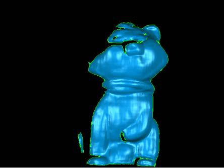
Sensors 2020, 20, 3718                                                                                     10 of 13

4. Discussions
     In regard to the accuracy of the proposed techniques, although the performance could be
further improved with much larger training datasets as well as deeper networks, preparing a
considerably large number of high-accuracy ground truth data is very time-consuming and challenging
at present. Furthermore, a deeper network will require a large amount of computer memory and
computational time for the learning process. Similarly, the proposed techniques are technically suitable
for high-resolution 3D shape reconstructions, but it is currently impractical because the learning time
would be substantially longer and a much larger memory size would be mandatory. The future
work can include exploring improved and advanced network models, preparing larger datasets
with a robot-aided process, developing less memory-consuming algorithms, and using sophisticated
central processing units (CPUs) and graphics processing units (GPUs) as well as cloud computing
services such as Amazon Web Services, Google Cloud, Microsoft Azure Cloud, and IBM Cloud [54–57].
Machine learning just gains popularity in the recent a few years, and it is reasonable to believe that the
aforementioned time-consuming and memory-consuming drawbacks will be lifted in the soon future.
     The deep machine learning models use multi-layer artificial neural networks to approach
the complex relationships between the captured images and physical quantities. Although the
unprecedented behaviors cannot be rigorously explained at present, more details will be revealed as
studies and investigations go further. The proposed techniques depend on using fringe-projection
images, but it will be worthy exploring networks and algorithms capable of working with other
kinds of structured-light images. Considering that the existing 3D imaging and shape measurement
techniques normally require complicated algorithms and relatively long computation time, the novel
3D imaging and shape measurement approaches based on artificial networks and deep machine
learning may have a considerable impact to the sensors and other relevant fields.

5. Conclusions
      In summary, a novel single-shot 3D shape reconstruction technique is presented. The approach
employs three deep CNN models, including FCN, AEN, and UNet, to quickly reconstruct the 3D
shapes from a single image of the target with a fringe pattern projected on it. The learning process is
accomplished through using the training and validation data acquired by a high-accuracy multi-shot
FPP technique. Experiments show that the UNet performs the best among the three networks.
The validity of the approach gives great promise in future research and development, which includes,
but not limited to, using larger datasets and less memory-consuming algorithms as well as conducting
a rigorous in-depth investigation on the CNN models.
      The measurement accuracy of the proposed technique is currently inferior to the existing prevalent
3D imaging and 3D shape reconstruction techniques. Nevertheless, its unprecedented behavior,
i.e., simple and robust, shows great potential in future high-performance 3D imaging. It could
remarkably broaden the capabilities and applications of the 3D imaging and shape reconstruction in
many fields of scientific research and engineering applications.

Supplementary Materials: The following two video clips are available online at www.mdpi.com/xxx/s1,
Video S1: Input images and their ground-truth labels of the training and test data, Video S2: Demonstration of the
intermediate results of the training process after each epoch.
Author Contributions: Conceptualization, Z.W. and H.N.; methodology, H.N. and Y.W.; software, H.N.;
validation, Y.W. and Z.W.; formal analysis, H.N. and Z.W.; data curation, H.N.; writing—original draft preparation,
H.N.; writing—review and editing, Z.W.; visualization, H.N.; supervision, Z.W. All authors have read and agreed
to the published version of the manuscript.
Funding: This research received no external funding.
Acknowledgments: The authors thank Thanh Nguyen at Instrument Systems & Technology Division, NASA for
helpful discussions on the CNN models. The authors are grateful to Hui Li and Qiang Qiu at RVBUST Inc. in
Shenzhen, China, for their valuable discussions and help on the experiments.
Conflicts of Interest: The authors declare no conflict of interest.
Sensors 2020, 20, 3718 11 of 13
References
1. Su, X.; Zhang, Q. Dynamic 3-D shape measurement method: A review. Opt. Lasers Eng. 2010, 48, 191–204.
[CrossRef]
2. Geng, J. Structured-light 3D surface imaging: A tutorial. Adv Opt. Photonics 2011, 2, 128–160. [CrossRef]
3. Zhang, S. High-speed 3D shape measurement with structured light methods: A review. Opt. Lasers Eng.
2018, 106, 119–131. [CrossRef]
4. Ma, Z.; Liu, S. A review of 3D reconstruction techniques in civil engineering and their applications.
Adv. Eng. Inf. 2018, 38, 163–174. [CrossRef]
5. Bräuer-Burchardt, C.; Heinze, M.; Schmidt, I.; Kühmstedt, P.; Notni, G. Underwater 3D Surface Measurement
Using Fringe Projection Based Scanning Devices. Sensors 2016, 16, 13. [CrossRef] [PubMed]
6. Du, H.; Chen, X.; Xi, J.; Yu, C.; Zhao, B. Development and Verification of a Novel Robot-Integrated Fringe
Projection 3D Scanning System for Large-Scale Metrology. Sensors 2017, 17, 2886. [CrossRef]
7. Liberadzki, P.; Adamczyk, M.; Witkowski, M.; Sitnik, R. Structured-Light-Based System for Shape
Measurement of the Human Body in Motion. Sensors 2018, 18, 2827. [CrossRef]
8. Cheng, X.; Liu, X.; Li, Z.; Zhong, K.; Han, L.; He, W.; Gan, W.; Xi, G.; Wang, C.; Shi, Y. Development and
Verification of a Novel Robot-Integrated Fringe Projection 3D Scanning System for Large-Scale Metrology.
Sensors 2019, 19, 668. [CrossRef]
9. Wu, H.; Yu, S.; Yu, X. 3D Measurement of Human Chest and Abdomen Surface Based on 3D Fourier
Transform and Time Phase Unwrapping. Sensors 2020, 20, 1091. [CrossRef]
10. Zuo, C.; Feng, S.; Huang, L.; Tao, T.; Yin, W.; Chen, Q. Phase shifting algorithms for fringe projection
profilometry: A review. Opt. Lasers Eng. 2018, 109, 2018. [CrossRef]
11. Zhang, S. Absolute phase retrieval methods for digital fringe projection profilometry: A review. Opt. Lasers
Eng. 2018, 107, 28–37. [CrossRef]
12. Zhu, J.; Zhou, P.; Su, X.; You, Z. Accurate and fast 3D surface measurement with temporal-spatial binary
encoding structured illumination. Opt. Express 2016, 25, 28549–28560. [CrossRef] [PubMed]
13. Cai, Z.; Liu, X.; Peng, X.; Yin, Y.; Li, A.; Wu, J.; Gao, B.Z. Structured light field 3D imaging. Opt. Express 2016,
24, 20324. [CrossRef] [PubMed]
14. Liu, X.; He, D.; Hu, H.; Liu, L. Fast 3D Surface Measurement with Wrapped Phase and Pseudorandom Image.
Sensors 2019, 19, 4185. [CrossRef]
15. Li, K.; Bu, J.; Zhang, D. Lens distortion elimination for improving measurement accuracy of fringe projection
profilometry. Opt. Lasers Eng. 2016, 86, 53–64. [CrossRef]
16. Li, B.; An, Y.; Zhang, S. Single-shot absolute 3D shape measurement with Fourier transform profilometry.
Appl. Opt. 2016, 55, 5219–5225. [CrossRef]
17. Zuo, C.; Tao, T.; Feng, S.; Huang, L.; Asundi, A.; Chen Q. Micro Fourier Transform Profilometry (µFTP):
3D shape measurement at 10,000 frames per second. Opt. Lasers Eng. 2018, 102, 70–91. [CrossRef]
18. Gorthi, S.; Rastogi, P. Fringe projection techniques: Whither we are? Opt. Lasers Eng. 2010, 48, 133–140.
[CrossRef]
19. Long, J.; Shelhamer, E.; Darrell, T. Fully Convolutional Networks for Semantic Segmentation. In Proceedings
of the IEEE Conference on Computer Vision and Pattern Recognition (CVPR), Boston, MA, USA,
7–12 June 2015.
20. Ronneberger, O.; Fischer, P.; Brox, T. U-Net: Convolutional Networks for Biomedical Image Segmentation.
In Intentional Conference on Medical Image Computing and Computer-Assisted Intervention (MICCAI); Springer:
Cham, Switzerland, 2015.
21. Badrinarayanan, V.; Kendall, A.; Cipolla, R. SegNet: A Deep Convolutional Encoder-Decoder Architecture
for Image Segmentation. IEEE Trans. Pattern Anal. Mach. Intell. 2017, 39, 2481–2495. [CrossRef]
22. Eigen, D.; Puhrsch, C.; Fergus, R. Depth Map Prediction from a Single Image Using a Multi-scale Deep
Network. In Proceedings of the International Conference on Neural Information Processing Systems (NIPS),
Montreal, QC, Canada, 8–11 December 2014.
23. Liu, F., Shen, C.; Lin, G. Deep convolutional neural fields for depth estimation from a single image.
In Proceedings of the IEEE Conference on Computer Vision and Pattern Recognition (CVPR), Boston,
MA, USA, 7–12 June 2015.Sensors 2020, 20, 3718 12 of 13
24. Choy, C.B.; Xu, D.; Gwak, J.; Chen, K.; Savarese, S. 3D-R2N2: A Unified Approach for Single and Multi-view
3D Object Reconstruction. In Proceedings of the European Conference on Computer Vision (ECCV),
Amsterdam, The Netherlands, 8–16 October 2016.
25. Dou, P.; Shah, S.; Kakadiaris, I. End-to-end 3D face reconstruction with deep neural network. In Proceedings
of the IEEE Conference on Computer Vision and Pattern Recognition (CVPR), Honolulu, HI, USA,
21–26 July 2017.
26. Paschalidou, D.; Ulusoy, A.; Schmitt, C.; Gool, L.; Geiger, A. RayNet: Learning Volumetric 3D Reconstruction
With Ray Potentials. In Proceedings of the IEEE Conference on Computer Vision and Pattern Recognition
(CVPR), Salt Lake City, UT, USA, 18–23 June 2018.
27. Feng, S.; Zuo, C.; Yin, W.; Gu, G.; Chen, Q. Micro deep learning profilometry for high-speed 3D surface
imaging. Opt. Lasers Eng. 2019, 121, 416–427. [CrossRef]
28. Feng, S.; Chen, Q.; Gu, G.; Tao, T.; Zhang, L.; Hu, Y.; Yin, W.; Zuo, C. Fringe pattern analysis using deep
learning. Adv. Photonics 2019, 1, 025001. [CrossRef]
29. Yin, W.; Chen, Q.; Feng, S.; Tao, T.; Huang, L.; Trusiak, M.; Asundi, A.; Zuo, C. Temporal phase unwrapping
using deep learning. Sci. Rep. 2019, 9, 20175. [CrossRef] [PubMed]
30. Jeught, S.; Dirckx, J. Deep neural networks for single shot structured light profilometry. Opt. Express 2019,
27, 17091–17101. [CrossRef] [PubMed]
31. Hao, F.; Tang, C.; Xu, M.; Lei, Z. Batch denoising of ESPI fringe patterns based on convolutional neural
network. Appl. Opt. 2019, 58, 3338–3346. [CrossRef] [PubMed]
32. Shi, J.; Zhu, X.; Wang, H.; Song, L.; Guo, Q. Label enhanced and patch based deep learning for phase retrieval
from single frame fringe pattern in fringe projection 3D measurement. Opt. Express 2019, 27, 28929–28943.
[CrossRef] [PubMed]
33. Yu, H.; Chen, X.; Zhang, Z.; Zuo, C.; Zhang, Y.; Zheng, D.; Han, J. Dynamic 3-D measurement based on
fringe-to-fringe transformation using deep learning. Opt. Express 2020, 28, 9405–9418. [CrossRef] [PubMed]
34. Stavroulakis, P.; Chen, S.; Delorme, C.; Bointon, P.; Tzimiropoulos, F.; Leach, R. Rapid tracking of extrinsic
projector parameters in fringe projection using machine learning. Opt. Lasers Eng. 2019, 114, 7–14. [CrossRef]
35. Ren, Z.; So, H.; Lam, E. Fringe Pattern Improvement and Super-Resolution Using Deep Learning in Digital
Holography. IEEE Trans. Ind. 2019, 15, 6179–6186. [CrossRef]
36. Yan, K. Yu, Y.; Huang, C.; Sui, L.; Qian, K.; Asundi, A. Fringe pattern denoising based on deep learning.
Opt. Commun. 2019, 437, 148–152. [CrossRef]
37. Lin, B.; Fu, S.; Zhang, C.; Wang, F.; Xie, S.; Zhao, Z.; Li, Y. Optical fringe patterns filtering based on multi-stage
convolution neural network. arXiv 2019, arXiv:1901.00361v1.
38. Figueroa, A.; Rivera, M. Deep neural network for fringe pattern filtering and normalization. arXiv 2019,
arXiv:1906.06224v1.
39. Hoang, T.; Pan, B.; Nguyen, D.; Wang, Z. Generic gamma correction for accuracy enhancement in
fringe-projection profilometry. Opt. Lett. 2010, 25, 1992–1994. [CrossRef] [PubMed]
40. Nguyen, H.; Wang, Z.; Quisberth, J. Accuracy Comparison of Fringe Projection Technique and 3D Digital
Image Correlation Technique. In Proceedings of the Conference Proceedings of the Society for Experimental
Mechanics Series (SEM), Costa Mesa, CA, USA, 8–11 June 2015.
41. Nguyen, H.; Nguyen, D.; Wang, Z.; Kieu, H.; Le, M. Real-time, high-accuracy 3D imaging and shape
measurement. Appl. Opt. 2015, 54, A9–A17. [CrossRef]
42. Nguyen, H.; Dunne, N.; Li, H.; Wang, Y.; Wang, Z. Real-time 3D shape measurement using 3LCD projection
and deep machine learning. Appl. Opt. 2019, 58, 7100–7109. [CrossRef] [PubMed]
43. Le, H.; Nguyen, H.; Wang, Z.; Opfermann, J.; Leonard, S.; Krieger, A.; Kang, J. Demonstration of a
laparoscopic structured-illumination three-dimensional imaging system for guiding reconstructive bowel
anastomosis. J. Biomed. Opt. 2018, 23, 056009. [CrossRef] [PubMed]
44. Wang, Z.; Nguyen, D.; Barnes, J. Some practical considerations in fringe projection profilometry.
Opt. Lasers Eng. 2010, 48, 218–225. [CrossRef]
45. Du, H.; Wang, Z. Three-dimensional shape measurement with an arbitrarily arranged fringe projection
profilometry system. Opt. Lett. 2007, 32, 2438–2440. [CrossRef]
46. Vo, M.; Wang, Z.; Hoang, T.; Nguyen, D. Flexible calibration technique for fringe-projection-based
three-dimensional imaging. Opt. Lett. 2010, 35, 3192–3194. [CrossRef]Sensors 2020, 20, 3718 13 of 13
47. Vo, M.; Wang, Z.; Pan, B.; Pan, T. Hyper-accurate flexible calibration technique for fringe-projection-based
three-dimensional imaging. Opt. Express 2012, 20, 16926–16941. [CrossRef]
48. Goodfellow, I.; Bengio, Y.; Courville, A. Deep Learning; The MIT Press: Cambridge, MA, USA, 2016.
49. Single-Shot 3D Shape Reconstruction Data Sets. Available online: https://figshare.com/articles/Single-
Shot_Fringe_Projection_Dataset/7636697 (accessed on 22 June 2020).
50. Kingma, D.; Ba, J. Adam: A Method for Stochastic Optimization. In Proceedings of the International
Conference on Learning Representations (ICLR), San Diego, CA, USA, 7–9 May 2015.
51. Wang, Z.; Kieu, H.; Nguyen, H.; Le, M. Digital image correlation in experimental mechanics and image
registration in computer vision: Similarities, differences and complements. Opt. Lasers Eng. 2015, 65, 18–27.
[CrossRef]
52. Nguyen, H.; Wang, Z.; Jones, P.; Zhao, B. 3D shape, deformation, and vibration measurements using infrared
Kinect sensors and digital image correlation. Appl. Opt. 2017, 56, 9030–9037. [CrossRef] [PubMed]
53. Nguyen, H.; Kieu, H.; Wang, Z.; Le, H. Three-dimensional facial digitization using advanced digital image
correlation. Appl. Opt. 2018, 57, 2188–2196. [CrossRef] [PubMed]
54. Amazon Web Services. Available online: https://aws.amazon.com (accessed on 22 June 2020).
55. Google Cloud: Cloud Computing Services. Available online: https://cloud.google.com (accessed on
22 June 2020).
56. Microsoft Azure: Cloud Computing Services. Available online: https://azure.microsoft.com/en-us
(accessed on 22 June 2020).
57. IBM Cloud. Available online: https://www.ibm.com/cloud (accessed on 22 June 2020).
c 2020 by the authors. Licensee MDPI, Basel, Switzerland. This article is an open access
article distributed under the terms and conditions of the Creative Commons Attribution
(CC BY) license (http://creativecommons.org/licenses/by/4.0/).You can also read