Determining Structural Properties of Artificial Neural Networks Using Algebraic Topology
←
→
Page content transcription
If your browser does not render page correctly, please read the page content below
Determining Structural Properties of Artificial Neural Networks
                                                             Using Algebraic Topology

                                             David Pérez Fernández* 1 , Asier Gutiérrez-Fandiño* 2 , Jordi Armengol-Estapé2 , and Marta
arXiv:2101.07752v2 [cs.LG] 21 Jan 2021

                                                                                         Villegas2
                                                                      1 Spanish Ministry of Inclusion, Social Security and Migration
                                                                         2 Text Mining Unit - Barcelona Supercomputing Center
                                                                                          1 david.perez@inv.uam.es
                                                                         2 {asier.gutierrez,jordi.armengol,marta.villegas}@bsc.es

                                                                                            January 22, 2021

                                         Abstract                                                       1    Introduction

                                         Artificial Neural Networks (ANNs) are widely used for
                                                                                                        Different types of ANNs can be trained for the same prob-
                                         approximating complex functions. The process that is usu-
                                                                                                        lem. Even for the same type of neural network, there
                                         ally followed to define the most appropriate architecture
                                                                                                        are many hyperparameters such as the number of neurons
                                         for an ANN given a specific function is mostly empirical.
                                                                                                        per layer or the number of layers. In addition, Stochastic
                                         Once this architecture has been defined, weights are usu-
                                                                                                        Gradient Descent (SGD) is a highly stochastic process.
                                         ally optimized according to the error function. On the other
                                                                                                        The final weights for the same set of hyperparameters can
                                         hand, we observe that ANNs can be represented as graphs
                                                                                                        vary, depending on the network initialization or the sample
                                         and their topological ’fingerprints’ can be obtained using
                                                                                                        training order.
                                         Persistent Homology (PH). In this paper, we describe a pro-
                                         posal focused on designing more principled architecture           The aim of this paper is to find invariants that can group
                                         search procedures. To do this, different architectures for     together neural networks trained for the same problem,
                                         solving problems related to a heterogeneous set of datasets    with independence of the particular architecture or initial-
                                         have been analyzed. The results of the evaluation corrobo-     ization. In this work, we focus on Fully Connected Neural
                                         rate that PH effectively characterizes the ANN invariants:     Networks (FCNNs) for the sake of simplicity. Given an
                                         when ANN density (layers and neurons) or sample feed-          ANN, we can represent it with a directed weighted graph.
                                         ing order is the only difference, PH topological invariants    It is possible to associate certain topological objects to
                                         hold; in the opposite direction, in different sub-problems     such graphs. See Jonsson [2007] for a complete reference
                                         (i.e. different labels), PH varies. This approach based on     on graph topology.
                                         topological analysis helps towards the goal of designing
                                         more principled architecture search procedures and having         We are using a special topological object from one topol-
                                         a better understanding of ANNs.                                ogy area named algebraic topology. In particular, as we
                                                                                                        said, we are experimenting with a topological object called
                                                                                                        Persistent Homology. For complete analysis of topological
                                           * Contributed   equally.                                     objects on graphs, see Aktas et al. [2019].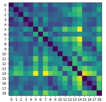
2    Related Work                                             Regarding ANN representation, one of the most related
                                                           works to ours, Gebhart et al. [2019], focuses on topolog-
One of the fundamental papers of Topological Data Anal-    ical neural network representation. They introduce a
ysis (TDA) is presented in Carlsson [2009] and suggests    method for computing PH over the graphical activation
the use of Algebraic Topology to obtain qualitative infor- structure of neural networks, which provides access to
mation and deal with metrics for large amounts of data. Forthe task-relevant substructures activated throughout the
an extensive overview of simplicial topology on graphs see network for a given input.
Giblin [1977], Jonsson [2007]. Aktas et al. [2019] provide    Interestingly, in Watanabe and Yamana [2020], authors
a thoroughly analysis of PH methods.                       work on ANN representation through simplicial complexes
   More recently, a number of publications have dealt with based on deep Taylor decomposition and they calculate
the study of the capacity of ANNs using PH. Guss and       the PH of ANNs in this representation. In Chowdhury
Salakhutdinov [2018b] characterize learnability of differ- et al. [2019], they use directed homology to represent
ent ANN architectures by computable measures of data       feed-forward fully connected neural network architectures.
complexity. Rieck et al. [2019b] introduce the neural per- They show that the path homology of these networks is
sistence metric, a complexity measure based on TDA on      non-trivial in higher dimensions and depends on the num-
weighted stratified graphs. Donier [2019] propose the con- ber and size of the network layers. They investigate homo-
cept of spatial capacity allocation analysis. Konuk and    logical differences between distinct neural network archi-
Smith [2019] propose an empirical study of how ANNs        tectures.
handle changes in topological complexity of the input data.
                                                              There has been a considerable growth of interest in
   In terms of pure ANN analysis, there are relevant works,
                                                           applied topology in the recent years. This popularity in-
like Hofer et al. [2020], that study topological regulariza-
                                                           crease and the development of new software libraries1 ,
tion. Clough et al. [2020] introduce a method for training
                                                           along with the growth of computational capabilities, have
neural networks for image segmentation with prior topol-
                                                           empowered new works. Some of the most remarkable
ogy knowledge, specifically via Betti numbers. Corneanu
                                                           libraries are Ripser (Tralie et al. [2018]), and Flagser
et al. [2020] estimate the performance gap between train-
                                                           (Lütgehetmann et al. [2019]). They are focused on the
ing and testing without the need of a testing dataset.
                                                           efficient computation of PH. For GPU-Accelerated compu-
   On the other hand, Topological analysis of decision
                                                           tation of Vietoris-Rips PH, Ripser++ (Zhang et al. [2020])
boundaries has been a very prolific area. Ramamurthy
                                                           offers a speedup of up to 30x in execution time with re-
et al. [2019] propose a labeled Vietoris-Rips complex to
                                                           spect to the original Ripser. The Python library we are
perform PH inference of decision boundaries for quantifi-
                                                           using, Giotto-TDA (Tauzin et al. [2020]), makes use of
cation of ANN complexity.
                                                           both above libraries underneath.
   Naitzat et al. [2020] experiment on the PH of a wide
range of point cloud input datasets for a binary classifica-  We contribute to the field of Topology applied to Deep
tion problems to see that ANNs transform a topologically   Learning by effectively characterizing ANNs using the
rich dataset (in terms of Betti numbers) into a topologi-  PH topological object, unlike other works (Corneanu et al.
cally simpler one as it passes through the layers. They    [2019], Guss and Salakhutdinov [2018a]) that approximate
also verify that the reduction in Betti numbers is signifi-neural networks representation in terms of input space.
cantly faster for ReLU activations than hyperbolic tangent In this way we provide a topological invariant that re-
activations.                                               late ANNs trained for similar problems, even if they have
   Liu [2020], they obtain certain geometrical and topo-   different architectures, and differentiate ANNs targeting
logical properties of decision regions for ANN models,     distinct problems. These topological properties are useful
and provide some principled guidance to designing and      for understanding the underlying topological complexity
regularizing ANNs. Additionally, they use curvatures of    and topological relationships of ANNs.
decision boundaries in terms of network weights, and the
rotation index theorem together with the Gauss-Bonnet-          1 https://www.math.colostate.edu/ adams/advising/
                                                                                                 ~
Chern theorem.                                               appliedTopologySoftware/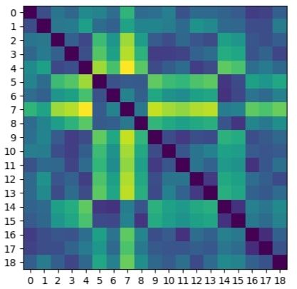
3      Methods
We obtain topological invariants associated to neural net-
works that solve a given problem. For doing so, we use the
PH of the graph associated to an ANN. We compute the PH
for various networks applied to different tasks. We then
compare all the diagrams for each one of the problems.
See the code2 for further details.

3.1      Experimental Settings
We start with some definitions on algebraic topology:
                                                                       Figure 1: Simplicial complex example
Definition 1 (simplex) A k-simplex is a k-dimensional
polytope which is the convex hull of its k + 1 vertices.
i.e. the set of all convex combinations λ0 v0 + λ1 v1 + ... +    We define the boundary, ∂ , as a function that maps i-
λk vk where λ0 + λ1 + ... + λk = 1 and 0 ≤ λ j ≤ 1 ∀ j ∈ simplex to the sum of its (i-1)-dimensional faces. Formally
{0, 1, ..., k}.                                               speaking, for an i-simplex σ = [v0 , . . . , vi ], its boundary
                                                              (∂ ) is:
Some examples of simplices are:                                                      i
                                                                             ∂i σ = ∑ [v0 , . . . , v̂ j , . . . , vi ]   (1)
    • 0-simplex is a point.                                                         j=0

     • 1-simplex is a line segment.                         where the hat indicates the v j is omitted.
                                                              We can expand this definition to i-chains. For an i-chain
   • 2-simplex is a triangle.                               c = ci σi , ∂i (c) = ∑i ci ∂i σi .
                                                              We can now distinguish two special types of chains
   • 3-simplex is a tetrahedron.
                                                            using the boundary map that will be useful to define ho-
Definition 2 (simplicial complex) A simplicial complex mology:
K is a set of simplices that satisfies the following condi-    • The first one is an i-cycle, which is defined as an
tions:                                                           i-chain with empty boundary. In other words, an
    1. Every subset (or face) of a simplex in K also belongs          i-chain c is an i-cycle if and only if ∂i (c) = 0, i.e.
       to K .                                                         c ∈ Ker(∂i ).

    2. For any two simplices σ1 and σ2 in K , if σ1 ∩ σ2 6= 0,
                                                            /      • An i-chain c is i-boundary if there exists an (i + 1)-
       then σ1 ∩ σ2 is a common subset, or face, of both σ1          chain d such that c = ∂i+1 (d), i.e. c ∈ Im(∂i+1 ).
       and σ2 .                                                    We associate to the ANN a weighted directed graph
                                                                 that is analyzed as a simplicial complex consisting on the
Definition 3 (directed flag complex) Let G = (V, E) be           union of points, axes, triangles, tetrahedrons and larger
a directed graph. The directed flag complex FC(G) is             dimension polytopes (those are the elements referred as
defined to be the ordered simplicial complex whose k-            simplices). As a formal definition of our central object,
simplices are all ordered (k + 1)-cliques, i.e., (k + 1)-        graphs:
tuples σ = (v0 , v1 , . . . , vk ), such that vi ∈ V ∀i, and Definition 4 (graph) A graph G is a pair (V, E), where
(vi , v j ) ∈ E for i < j.                                   V is a finite set referred to as the vertices or nodes of
    2 https://github.com/PlanTL-SANIDAD/                     G, and E is a subset of the set of unordered pairs e =
net-homology-properties                                      {u, v} of distinct points in V , which we call the edges of G.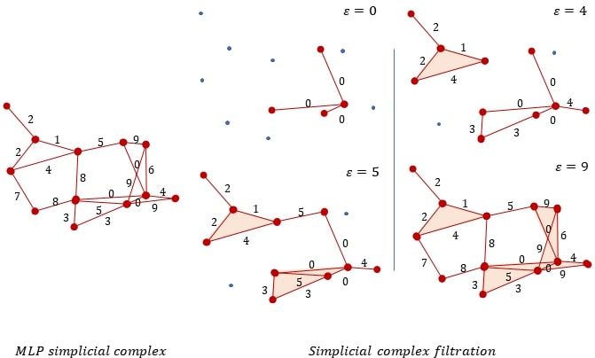
Geometrically the pair {u, v} indicates that the vertices u       This quotient space is called i-th homology group of the
and v are adjacent in G. A directed graph, or a digraph, is       simplicial complex K:
similarly a pair (V, E) of vertices V and edges E, except                                   Zi (K)   Ker(∂i )
the edges are ordered pairs of distinct vertices, i.e.,the pair                  Hi (K) =          =                        (3)
                                                                                            Bi (K) Im(∂i+1 )
(u, v) indicates that there is an edge from u to v in G. In
a digraph, we allow reciprocal edges, i.e., both (u, v) and       where Ker and Im are the function kernel and image re-
(v, u) may be edges in G, but we exclude loops, i.e., edges       spectively.
of the form (v, v).                                                 The dimension of i-th homology is called the i-th Betti
                                                                  number of K, βi (K), where:
   Given a trained ANN, we take the collection of network
                                                                           βi (K) = dim(Ker(∂i )) − dim(Im(∂i+1 ))          (4)
connections as directed and weighted edges that join neu-
rons, represented by graph nodes. Biases are considered as           The i-th Betti number is the number of i-dimensional
new edges that join new vertices, with a source neuron that       voids in the simplicial complex (β0 gives the number of
has a given weight. Note that in this representation we lose      connected components of the simplicial complex, β1 gives
the information about the activation functions, for simplic-      the number of loops and so on). For a deeper introduction
ity and to avoid representing the network as a multiplex          to algebraic topology and computational topology, we refer
network. Bias information could also have been ignored            to Edelsbrunner and Harer [2009], Ghrist [2014].
because, as we will see, it is not very informative in terms         We are going to work with a family of simplicial com-
of topology.                                                      plexes, K ε , for a range of values of ε ∈ R so that the
   For negative edge weights, we decide to reverse edge           complex at step εt is embedded in the complex at εt+1 for
directions and maintain the absolute value of the weights.        εt ≤ εt+1 , i.e. Kε ⊆ Kεt+1 . This nested family of simplicial
We discard the use of weight absolute value as ANNs are           complexes is called a filtration.
not invariant under weight sign transformations. We also
decided not to use PH interval [min(weight), max(weight)],
when min(weight) < 0, because the treatment of zero value
is not topologically coherent.
   We then normalize the weights of all the edges as ex-
pressed in Equation 2 where w is the weight to normalize,
W are all the weights and ζ is an smoothing parameter that
we set to 0.000001. This smoothing parameter is necessary
as we want to avoid normalized weights of edges to be 0.
This is because 0 implies a lack of connection.

                             |w|
          max(1 −                             ,ζ)          (2)
                    max(|max(W )|, |min(W )|)
   Given a weighted directed graph obtained from a trained               Figure 2: Simplicial complex filtration
ANN, we define a directed flag complex associated to it.
   Next we define the topological object that we will use to     Given a filtration, one can look at the birth, where a ho-
analyze the directed flag complex associated with neural mology object appears, and death, the time where the hole
networks.                                                     disappears. The PH treats the birth and the death of these
                                                              homological features in Kε for different ε values. Lifes-
Definition 5 (homology group) Given these two special pan of each homological feature can be represented as an
subspaces, i-cycles Zi (K) and i-boundaries Bi (K) of Ci (K), interval, (birth, death), of the homological feature. Given
we now take the quotient space of Bi (K) as a subset of a filtration, one can record all these intervals by a Persis-
Zi (K). In this quotient space, there are only the i-cycles tence Barcode (PB) (Carlsson [2009]), or in a Persistence
that do not bound an (i + 1)-complex, or i-voids of K. Diagram (PD), as a collection of multiset of intervals.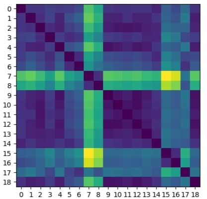
For the simplicial complex associated to ANN directed                  For our topological calculations (persistence homology,
weighted graph, we use as ε filtration parameter the                   discretization, and diagram distance calculation) we used
edge weight. This filtration gives a collection of con-                Giotto-TDA (Tauzin et al. [2020]) and the following sup-
tained directed weighted graph or simplicial complex                   ported vectorized persistence summaries: • Persistence
Kεmin . . . Kεt ⊆ Kεt+1 . . . Kεmax , where t ∈ [0, 1] and εmin = 0,   landscape. • Weighted silhouette. • Heat vectorizations.
εmax = 1 (remember that edge weights are normalized).
   As mentioned previously, our interest in this paper is              Definition 7 (Persistence landscape) Given a collection
to compare PDs from two different simplicial complex.                  of intervals {(bi , di )}i∈I that compose a PD, its persistence
There are two distances traditionally used to compare PDs,             landscape is the set of functions λk : R → R defined by
Wasserstein distance and Bottleneck distance. Their stabil-            letting λk (t) be the k-th largest value of the set {Λi (t)}i∈I
ity with respect to perturbations on PDs has been object of            where:
different studies (Chazal et al. [2012], Cohen-Steiner et al.                          Λi (t) = [min{t − bi , di − t}]+            (7)
[2005]).
   In order to make computations feasible, we filter the               and c+ := max(c, 0). The function λk is referred to as the
PDs by limiting the minimum interval size. We do so by                 k-layer of the persistence landscape.
setting a threshold η = 0.01. Additionally, for computing                 Now we define a vectorization of the set of real-valued
distances, we need to remove infinity values. As we are                function that compose PDs on N × R. For any p = 1, . . . , ∞
only interested in the deaths until the maximum weight                 we can restrict attention to PDs D whose associated per-
value, we replace all the infinity values by 1.0.                      sistence landscape λ is p-integrable, that is to say,
Definition 6 (Wasserstein distance) The p-Wasserstein                                                  !1/p
distance between two PDs D1 and D2 is the infimum over                                               p
                                                                                ||λ || p = ∑ ||λi || p                (8)
all bijections: γ : D1 → D2 of:                                                            i∈N
                                            1/p
           dW (D1 , D2 ) = ∑ ||x − γ(x)||∞p               (5) is finite. In this case, we refer to Equation (8) as the p-
                              x∈D1                            landscape norm of D. For p = 2, we define the value of
                                                              the landscape kernel or similarity of two vectorized PDs D
where || − ||∞ is defined for (x, y) ∈ R2 by max{|x|, |y|}. and E as
The limit p → ∞ defines the Bottleneck distance. More
                                                                                                            !1/2
explicitly, it is the infimum over the same set of bijections                            Z
                                                                                                          2
of the value                                                            hλ , µi = ∑ |λi (x) − µi (x)| dx              (9)
                                                                                            i∈N R
               dB (D1 , D2 ) = sup ||x − γ(x)||∞ .              (6)
                               x∈D1
                                                              where λ and µ are their associated persistence land-
   The set of PDs together with any of the distances de- scapes.
scribed above is a metric space. We work on this metric
space to analyze the similarity between simplicial com- λk is geometrically described as follows. For each i ∈ I, we
plexes associated to neural networks.                         draw an isosceles triangle with base the interval (bi , di ) on
   In order to apply PDs distance to real cases, we need to the horizontal t-axis, and sides with slope 1 and −1. This
make calculations computationally feasible. Wasserstein subdivides the plane into a number of polygonal regions
distance calculations are computationally hard for large that we label by the number of triangles contained on it. If
PDs (each PD of our ANN models has a million persistence Pk is the union of the polygonal regions with values at least
intervals per diagram). We will use a vectorized version k, then the graph of λk is the upper contour of Pk , with
of PDs, also called PD discretization. This vectorized λk (a) = 0 if the vertical line t = a does not intersect Pk .
version summaries have been proposed and used on recent
literature (Adams et al. [2017], Berry et al. [2020], Bubenik Definition 8 (Weighted silhouette) Let D = {(bi , di )}i∈I
[2015], Lawson et al. [2019], Rieck et al. [2019a]).          be a PD and w = {wi }i∈I a set of positive real numbers.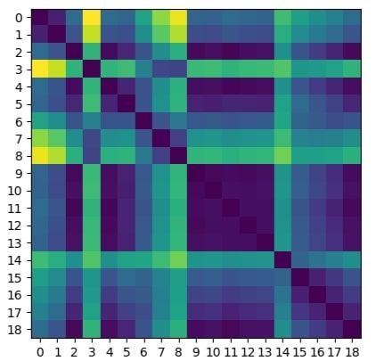
The silhouette of D weighted by w is the function φ : R → R 3.2 Datasets
defined by:
                            ∑ wi Λi (t)                       To determine the topological structural properties of
                    φ (t) = i∈I           ,              (10) trained ANNs, we select different kinds of datasets. We opt
                               ∑i∈I wi
                                                              for three well-known benchmarks in the machine learning
where                                                         community: (1) the MNIST4 dataset for classifying hand-
               Λi (t) = [min{t − bi , di − t}]+          (11) written digit images, (2) the CIFAR-105 (CIFAR) dataset
                                                              for classifying ten different objects, (3) and the Language
and c+ := max(c, 0) When wi = |di − bi | p for 0 < p ≤ ∞
                                                              Identification Wikipedia dataset6 for classifying 7 different
we refer to φ as the p-power-weighted silhouette of D. It
                                                              languages.
defines a vectorization of the set of PDs on the vector space
                                                                 We selected the MNIST dataset since it is based on
of continuous real-valued functions on R.
                                                              images but, at the same time, it does not require a CNN
                                                              to obtain competitive results. For this dataset, we only
Definition 9 (Heat vectorizations) Considering PD as
                                                              used a Fully Connected Neural Network with Dropout. On
the support of Dirac deltas, one can construct, for any
                                                              the other hand, CIFAR, a more difficult benchmark, re-
t > 0, two vectorizations of the set of PDs to the set of
                                                           2  quires a CNN for obtaining good enough accuracy. Since
continuous real-valued function on the first quadrant R>0 .
                                                              our method does not contemplate CNNs weights, differ-
The heat vectorization is constructed for every PD D by
                                                              ent trainings could provide noisy diagrams. To avoid this
solving the heat equation:
                                                              issue, we first train a CNN, and then we keep its convolu-
                                                              tional feature extractor. Finally, we train all the networks
        ∆x (u) = ∂t u      on Ω × R>0                         with the same convolutional feature extractor by freezing
                                                              the convolutional weights. In the case of the Language
             u=0           on {x1 = x2 } × R≥0
                                                         (12) Identification dataset, it is a textual dataset that requires
             u = ∑ δ p on Ω × 0                               vectorizing (in this case, with character frequency), and
                  p∈D
                                                              the vectors are fed to a FCNN.
where Ω = {(x1 , x2 ) ∈ R2 | x1 ≤ x2 }, then solving the
same equation after precomposing the data of Equation               3.3     Experiments Pipeline
(12) with the change of coordinates (x1 , x2 ) 7→ (x2 , x1 ), and
defining the image of D to be the difference between these We study the following variables (hyperparameters):
two solutions at the chosen time t.                        1. Layer width, 2. Number of layers, 3. Input order7 ),
    We recall that the solution to the heat equation with  4. Number of labels (number of considered classes).
initial condition given by a Dirac delta supported at p ∈ R2  We define the base architecture as the one with a layer
is:                                                        width of 512, 2 layers, the original features order, and
                    1

                                ||p − x||2
                                                          considering all the classes (10 in the case of MNIST and
                       exp −                                 (13)
                                                           CIFAR, and 7 in the case of the language identification
                   4πt              4t
                                                           task). Then, doing one change at a time, keeping the rest
To highlight the connection with normally distributed ran- of the base architecture hyperparameters, we experiment
dom variables,√ it is customary to use the the change of with architectures with the following configurations:
variable σ = 2t.
                                                              • Layer width: 128, 256, 512 (base) and 1024.
  For a complete reference on vectorized persistence sum-     4 http://yann.lecun.com/exdb/mnist/
maries and PH approximated metrics, see Tauzin et al.         5 https://www.cs.toronto.edu/ kriz/cifar.html
                                                                                            ~
[2020], Berry et al. [2020] and Giotto-TDA package docu-      6 https://www.floydhub.com/floydhub/datasets/

mentation appendix3 .                                      language-identification/1/data
                                                                       7 Order of the input features. This one should definitely not affect the
   3 https://giotto-ai.github.io/gtda-docs/0.3.1/                   performance in an fully-connected neural network, so if our method is
theory/glossary.html#persistence-landscape                          correct, it should be uniform as per the proposed topological metrics.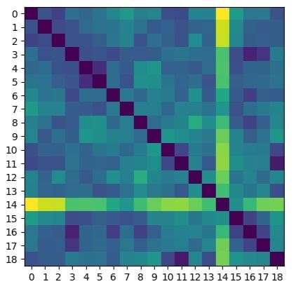
• Number of layers: 2 (base), 4, 6, 8 and 10. than the Landscape distance matrix of Figure 3c. Heat and
Silhouette distance matrices, unlike the Landscape one,
• Input order: 5 different randomizations (with base make distinguishing the groups of experiments straightfor-
structure). ward. In both the Heat and Silhouette distance matrices,
the increases in layer size imply gradual differences in the
• Number of labels (MNIST, CIFAR): 2, 4, 6, 8 and
topological distances. The same holds for the number of
10 (base).
layers, and number of labels. This means that the increase
• Number of labels (Language Identification): 2, 3, 4, in the network capacity directly maps to the increase in
6 and 7 (base). topological complexity. The input order slightly alters
the topological space but with no interpretable topological
Note that this is not a grid search over all the combinations. meaning.
We always modify one hyperparameter at a time, and keep Results of experiments in CIFAR datasets are shown in
the rest of them as in the base architecture. In other words, second row of Figure 3. CIFAR dataset results are inter-
we experiment with all the combinations such that only estingly different from those of MNIST dataset. This is,
one of the hyperparameters is set to a non-base value at a presumably, because the CIFAR uses a pretrained CNN on
time. the ten classes of the problem. Thus, we should understand
For each dataset, we train 5 times (each with a dif- the results from this context.
ferent random weight initialization) each of these neural As shown in Figures 3d and 3e, in the Heat and Silhou-
network configurations. Then, we compute the topologi- ette distance matrices, increasing the layer size implies a
cal distances (persistence landscape, weighted silhouette, gradual increase in topological distance. The first fully
heat) among the different architectures. In total, we obtain connected layer size is important as it can avoid a bottle-
3 × 5 × 3× distance matrices (3 datasets, 5 random initial- neck from the previous CNN output. Some works in the
izations, 3 distance measures). Finally, we average the 5 literature show that adding multiple fully connected layers
random initializations, such that we get 3 × 3 matrices, one does not necessarily enhance the prediction capability of
for each distance on each dataset. All the matrices have CNNs (Basha et al. [2019]), which is congruent with our
dimensions 19 × 19, since 19 is the number of experiments results when adding fully connected layers. Furthermore,
for each dataset (corresponding to the total the number experiments regarding the number of labels of the network
of architectural configurations mentioned above). Note remain close in distance. This could provide additional
that the base architecture appears 8 times (1, on the num- support to the theory that adding more FCN layers do
ber of neurons per layer, 1 on the number of layers, 1 on not enhance CNNs prediction capabilities, and also to the
the number of labels and the 5 randomizations of weight claim that the CNN is the main feature extractor of the
initializations). network (and the FCNN only works as a pure classifier).
Concerning the experiments of input order, in this case
there is slightly more homogeneity than in MNIST, again
4 Results Analysis & Discussion showing that the order of sample has negligible influence.
Moreover, there could have been even more homogeneity
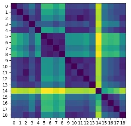
Figure 3 provides the results for each dataset and for each taking into account that the fully connected network re-
one of the distance metrics. On the bottom of the figure, duced its variance thanks to the frozen weights of the CNN.
the experiments indices and experiments are related. The This also supports the fact that the CNN is the main feature
results shown in the figure are positive for the validation of extractor of the network. As in MNIST results, CIFAR
our method, since most of the experiment groups are triv- results show that the topological properties are surprisingly
ially distinguishable. Note that the matrices are symmetric a mapping of the practical properties of ANNs.
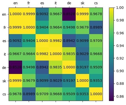
and that the diagonal is all zeros. As for the Language Identification dataset with charac-
In the first row of Figure 3 from the MNIST dataset, the ters, Figures 3g and 3h indicate that increasing the layer
Heat distance matrix shown in Figure 3a and Silhouette size results in topological distance increase. However, un-
distance matrix shown in Figure 3b look more informative like in the two previous datasets, introducing more layers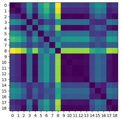
(a) MNIST - Heat.                        (b) MNIST - Silhouette.                    (c) MNIST - Landscape.

           (d) CIFAR - Heat.                        (e) CIFAR - Silhouette.                     (f) CIFAR - Landscape.

   (g) Language Identification - Heat.      (h) Language Identification - Silhouette.   (i) Language Identification - Landscape.

Experiment indices                         Experiment
                                     0-3   Layer sizes.
                                     4-8   Number of layers.
                                    9-13   Input ordering.
                                   14-18   Number of labels.

               Figure 3: Distance matrices of all network architectures presented. Average of 5 runs.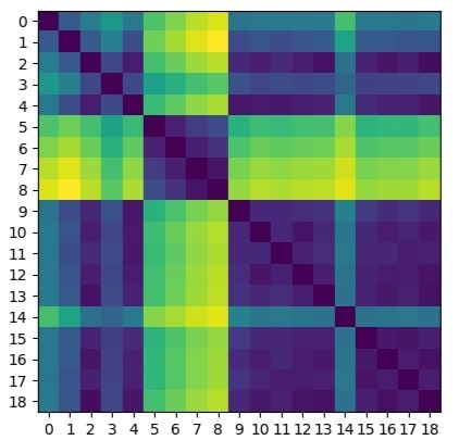
does not derive in a gradual topological distance increase.
Although it tends to a gradual increase, there are gaps or
unexpected peaks that avoid this gradual increase from hap-
pening. This might be related to overfitting as the network
with larger capacity memorizes the training samples and,
therefore, it deviates from a correct problem generalization.
In other words, there might be sample memorization. This
happens in the Language Identification dataset and does
not in the two vision ones because this one is simpler to
learn (e.g., in this case, a plain Multi-Layer Perceptron
with one hidden layer classifier is already competitive).
Regarding the sample shuffling, as in the previous datasets
there is small distance among all experiments with no            Figure 4: Language Identification dataset cosine similar-
noticeable variation.                                            ity of the sum of all character vectors for each language
   Finally, for the experiments of number of labels, we hy-      normalized.
pothesize that experiments appear to be noisy due to (1) the
similarity and dissimilarity of languages, (2) the increase
in the complexity of the problem, (3) more labels help to        might be due to the large inter-cluster distances; the learn-
enhance the understanding of the problem representation,         ing structure changes dramatically in those cases. The
and (4) label imbalance will make large languages to be          Silhouette distance matrix of Figure 3h is slightly more
more accurately recognized. While (1) and (4) add some-          strict about computing similarities. In other words, only
how expected noise as languages are arbitrarily ordered,         very close items appear to be similar. Adding labels up to
(2) makes ANN complexity to be larger with more labels           Spanish and up to Italian show strong similarity.
and, in contrary, (3) decreases the complexity of the ANN
as the understanding of the problem is deeper with more
labels. Languages are sorted as English, French, Spanish,        5    Conclusions & Future Work
Italian, German, Slovenian and Czech. In principle, one
would say that English and German are similar as they are        Results from different experiments, in three different
Germanic languages; Spanish, Italian and French are simi-        datasets from computer vision and natural language, lead
lar as they are Romance languages; Slovenian and Czech           to similar topological structural properties and are trivially
are similar as they are Slavic languages. Nevertheless,          interpretable, which yields to general applicability.
one must take into account classifier is based on character         The bests discretizations chosen for this work are the
frequencies, so the intuitive closeness of languages does        Heat and Silhouette. They show better separation of ex-
not necessarily hold. This can be checked by comparing           periment groups (invariants), and are effectively reflecting
the cosine similarity of the character frequencies vector of     changes in a sensible way. On the other hand, we also
each language. See Figure 4 for further details.                 explored the Landscape discretization but it offers a very
   In the Heat distance matrix of Figure 3g, when increas-       low interpretability and clearance. In other words, it is not
ing from two labels to three, we observe that the gap when       helpful for comparing PH diagrams associated to ANNs.
adding Spanish is larger than when adding Spanish and               The selected ANN representation is reliable and com-
Italian, as Italian is very close to English and French, while   plete, and yields coherent and realistic results. Currently,
Spanish is far away. Adding German and Slovenian in-             our representation system is applicable to Fully Connected
creases the difference, presumably because of the large          layers. However, most popular Deep Learning libraries do
differences that Slovenian has with the rest of the lan-         not include neither graph representation tools nor consis-
guages. Two hubs are easily distinguishable, the one with        tent computation graph traversing utilities which makes
Romance languages plus English and the other one with            ANN graph representation harder.
the one with Slavic languages plus German. Differences              As future work, we are planning to adapt to low-level
Deep Learning libraries and to support popular ANN ar-       of Applied and Computational Topology, 4:211–262,
chitectures such as CNNs, Recurrent Neural Networks,         2020.
and Transformers (Vaswani et al. [2017]). Furthermore,
we would like to come up with a universal neuron-level P. Bubenik. Statistical topological data analysis using
computing graph representation.                              persistence landscapes. J. Mach. Learn. Res., 16:77–
   Following the ANN representation concern, we would        102, 2015.
additionally like to represent the ANNs node types and
operations more concretely in the graph. We are also G. Carlsson. Topology and data. Bulletin of the American
working on these representations; the main challenge is      Mathematical Society, 46:255–308, 2009.
to avoid representing the network as a multiplex network.
We are performing more analysis regarding the learning of F. Chazal, V. D. Silva, and S. Oudot. Persistence stability
an ANN, and trying to topologically answer the question      for geometric complexes. Geometriae Dedicata, 173:
of how an ANN learns.                                        193–214,  2012.

                                                            S. Chowdhury, T. Gebhart, S. Huntsman, and M. Yutin.
Acknowledgements                                               Path homologies of deep feedforward networks. 2019
                                                               18th IEEE International Conference On Machine Learn-
We want to thank David Griol Barres, Jerónimo Arenas-         ing And Applications (ICMLA), pages 1077–1082, 2019.
Garcı́a and Esther Ibáñez-Marcelo for their review, feed-
back and corrections on the paper.                          J. Clough, I. Öksüz, N. Byrne, V. Zimmer, J. A. Schn-
   This work was funded by the Spanish State Secretariat       abel, and A. P. King. A topological loss function for
for Digitalization and Artificial Intelligence to carry out    deep-learning based image segmentation using persis-
support activities in supercomputing within the framework      tent homology. IEEE transactions on pattern analysis
               8
of the PlanTL signed on 14 December 2018.                      and machine intelligence, PP, 2020.

                                                            D. Cohen-Steiner, H. Edelsbrunner, and J. Harer. Stability
                                                              of persistence diagrams. Proceedings of the twenty-first
References                                                    annual symposium on Computational geometry, 2005.
H. Adams, T. Emerson, M. Kirby, R. Neville, C. Peterson,
                                                          C. Corneanu, M. Madadi, S. Escalera, and A. Martı́nez.
  P. Shipman, S. Chepushtanova, E. Hanson, F. Motta,
                                                            Computing the testing error without a testing set. 2020
  and L. Ziegelmeier. Persistence images: A stable vector
                                                            IEEE/CVF Conference on Computer Vision and Pattern
  representation of persistent homology. J. Mach. Learn.
                                                            Recognition (CVPR), pages 2674–2682, 2020.
  Res., 18:8:1–8:35, 2017.
M. Aktas, E. Akbaş, and A. E. Fatmaoui. Persistence ho- C. A. Corneanu, M. Madadi, S. Escalera, and A. M. Mar-
   mology of networks: methods and applications. Applied      tinez. What does it mean to learn in deep networks?
   Network Science, 4:1–28, 2019.                             and, how does one detect adversarial attacks? In 2019
                                                              IEEE/CVF Conference on Computer Vision and Pat-
S. H. S. Basha, S. R. Dubey, V. Pulabaigari, and S. Mukher-   tern Recognition (CVPR), pages 4752–4761, 2019. doi:
   jee. Impact of fully connected layers on performance       10.1109/CVPR.2019.00489.
   of convolutional neural networks for image classifi-
   cation. CoRR, abs/1902.02771, 2019. URL http: J. Donier. Capacity allocation analysis of neural net-
   //arxiv.org/abs/1902.02771.                                works: A tool for principled architecture design. ArXiv,
                                                              abs/1902.04485, 2019.
E. Berry, Y.-C. Chen, J. Cisewski-Kehe, and B. T. Fasy.
   Functional summaries of persistence diagrams. Journal
                                                            H. Edelsbrunner and J. Harer. Computational Topology -
   8 https://www.plantl.gob.es/                               an Introduction. American Mathematical Society, 2009.
T. Gebhart, P. Schrater, and A. Hylton. Characterizing K. Ramamurthy, K. R. Varshney, and K. Mody. Topologi-
the shape of activation space in deep neural networks. cal data analysis of decision boundaries with application
2019 18th IEEE International Conference On Machine to model selection. ArXiv, abs/1805.09949, 2019.
Learning And Applications (ICMLA), pages 1537–1542,
2019. B. A. Rieck, F. Sadlo, and H. Leitte. Topological machine
learning with persistence indicator functions. ArXiv,
R. Ghrist. Elementary Applied Topology. Self-published, abs/1907.13496, 2019a.
2014.
B. A. Rieck, M. Togninalli, C. Bock, M. Moor, M. Horn,
P. Giblin. Graphs, surfaces, and homology : an introduc- T. Gumbsch, and K. Borgwardt. Neural persistence:
tion to algebraic topology. Chapman and Hall, 1977. A complexity measure for deep neural networks using
algebraic topology. ArXiv, abs/1812.09764, 2019b.
W. H. Guss and R. Salakhutdinov. On characterizing the
G. Tauzin, U. Lupo, L. Tunstall, J. B. Pérez, M. Caorsi,
capacity of neural networks using algebraic topology.
A. Medina-Mardones, A. Dassatti, and K. Hess. giotto-
CoRR, abs/1802.04443, 2018a. URL http://arxiv.
tda: A topological data analysis toolkit for machine
org/abs/1802.04443.
learning and data exploration, 2020.
W. H. Guss and R. Salakhutdinov. On characterizing the C. Tralie, N. Saul, and R. Bar-On. Ripser.py: A lean
capacity of neural networks using algebraic topology. persistent homology library for python. The Jour-
ArXiv, abs/1802.04443, 2018b. nal of Open Source Software, 3(29):925, Sep 2018.
doi: 10.21105/joss.00925. URL https://doi.org/
C. Hofer, F. Graf, M. Niethammer, and R. Kwitt. Topolog-
10.21105/joss.00925.
ically densified distributions. ArXiv, abs/2002.04805,
2020. A. Vaswani, N. Shazeer, N. Parmar, J. Uszkoreit, L. Jones,
A. N. Gomez, L. Kaiser, and I. Polosukhin. Attention
J. Jonsson. Simplicial complexes of graphs. PhD thesis,
is all you need. CoRR, abs/1706.03762, 2017. URL
KTH Royal Institute of Technology, 2007.
http://arxiv.org/abs/1706.03762.
E. Konuk and K. Smith. An empirical study of the relation S. Watanabe and H. Yamana. Topological measurement
between network architecture and complexity. 2019 of deep neural networks using persistent homology. In
IEEE/CVF International Conference on Computer Vi- ISAIM, 2020.
sion Workshop (ICCVW), pages 4597–4599, 2019.
S. Zhang, M. Xiao, and H. Wang. Gpu-accelerated compu-
P. Lawson, A. Sholl, J. Brown, B. T. Fasy, and C. Wenk. tation of vietoris-rips persistence barcodes. In Sympo-
Persistent homology for the quantitative evaluation of sium on Computational Geometry, 2020.
architectural features in prostate cancer histology. Sci-
entific Reports, 9, 2019.
B. Liu. Geometry and topology of deep neural networks’
decision boundaries. ArXiv, abs/2003.03687, 2020.
D. Lütgehetmann, D. Govc, J. Smith, and R. Levi. Com-
puting persistent homology of directed flag complexes.
arXiv: Algebraic Topology, 2019.
G. Naitzat, A. Zhitnikov, and L. Lim. Topology of deep
neural networks. J. Mach. Learn. Res., 21:184:1–184:40,
2020.You can also read