A Framework to Learn with Interpretation - arXiv.org
←
→
Page content transcription
If your browser does not render page correctly, please read the page content below
A Framework to Learn with Interpretation
                                                                  Jayneel Parekh 1 , Pavlo Mozharovskyi 1 , Florence d’Alché-Buc 1
                                                                                  1
                                                                                   LTCI, Telecom Paris, Institut Polytechnique de Paris
                                                                        {jayneel.parekh, pavlo.mozharovskyi, florence.dalche}@telecom-paris.fr
arXiv:2010.09345v2 [cs.LG] 13 Jan 2021

                                                                     Abstract                                 sophisticated frameworks (Dubois and Prade 2014; Guidotti
                                                                                                              et al. 2019). To address the long-standing challenge of in-
                                           With increasingly widespread use of deep neural networks in        terpreting black-box models such as deep neural networks
                                           critical decision-making applications, interpretability of these
                                                                                                              (Samek et al. 2019; Beaudouin et al. 2020; Barredo Arrieta
                                           models is becoming imperative. We consider the problem of
                                           jointly learning a predictive model and its associated inter-      et al. 2020), two main approaches have been developed in
                                           pretation model. The task of the interpreter is to provide both    literature: post-hoc approaches and “by design methods”.
                                           local and global interpretability about the predictive model           Post-hoc approaches like saliency maps (Springenberg
                                           in terms of human-understandable high level attribute func-        et al. 2014; Selvaraju et al. 2017) and perturbation based
                                           tions, without any loss of accuracy. This is achieved by a         methods (Lundberg and Lee 2017) address the interpretabil-
                                           dedicated architecture and well chosen regularization penal-       ity issue by considering a trained network and analyze a pos-
                                           ties. We seek for a small-size dictionary of attribute functions   teriori its behavior by performing attribution over input fea-
                                           that take as inputs the outputs of selected hidden layers and
                                           whose outputs feed a linear classifier. We impose a high level
                                                                                                              tures or building a local proxy model, generally linear, in
                                           of conciseness by constraining the activation of a very few at-    the vicinity of a datapoint. While these approaches have un-
                                           tributes for a given input with a real-entropy-based criterion     doubtedly increased the understanding of a network’s deci-
                                           while enforcing fidelity to both inputs and outputs of the pre-    sion, they fail to capture a global picture and are criticized
                                           dictive model. A major advantage of simultaneous learning          for not explaining the predictor function itself.
                                           is that the predictive neural network benefits from the inter-         This drawback is alleviated by another line of research,
                                           pretability constraint as well. We also develop a more detailed    “interpretability by design” (Al-Shedivat, Dubey, and Xing
                                           pipeline based on some common and novel simple tools to
                                                                                                              2017; Melis and Jaakkola 2018), which aims at integrating
                                           develop understanding about the learnt features. We show on
                                           two datasets, MNIST and QuickDraw, their relevance for both        the interpretability objective in the learning process. This
                                           global and local interpretability.                                 long-standing approach modifies the structure of predictor
                                                                                                              function itself to make it equivalent to a set of logical rules
                                                                                                              and/or adds to the loss function regularizing penalties to en-
                                                                 Introduction                                 force interpretability. Although the literature has not reached
                                         Owing to the high competitive performance, machine learn-            a consensus on these properties, one can mention consis-
                                         ing methods and specially deep neural networks have re-              tency, completeness, stability and sparsity. However, in this
                                         cently made major inroads in classification and decision-            attractive family of approaches, the interpretability is often
                                         making applications. However their deployment in critical            paid at the expense of accuracy. The goal of this work is
                                         environments such as applications in defence, law, health-           to propose and study a novel framework to learning inter-
                                         care or any domain that has a high impact on human lives             pretable networks while overcoming the trade-off between
                                         has strongly induced the need to understand the “rationale”          accuracy and interpretability. Our starting point rely upon
                                         behind their decisions. This has even led to impose inter-           two notions of interpretability: for a given input, local in-
                                         pretability and explainability of these systems as part of le-       terpretability is the ability of a model to provide a small
                                         gal and human rights (see General Data Protection Regula-            subset of high level attributes, whose simultaneous activa-
                                         tion1 ). It is important to stress that explainability as well as    tion leads to the model’s prediction. Global interpretability
                                         interpretability are often used as synonyms in the literature,       corresponds here to the whole picture, i.e. the different sets
                                         referring to the ability to provide human-understandable in-         of attributes that are associated to class prediction. In our
                                         sights on the decision process. Throughout this paper, we opt        novel approach called FLINT (Framework for Learning In-
                                         for interpretability as in (Doshi-Velez and Kim 2017) and            terpretable Networks), we consider a pair of models, a pre-
                                         leave the term explainability for the ability to provide log-        dictor network, and an interpreter network, whose architec-
                                         ical explanations or causal reasoning, both requiring more           tures are closely linked, and that are jointly learned. There is
                                                                                                              no strong assumption on the predictor network, except that
                                         Preprint, paper under review                                         it is a deep architecture and thus it is able to learn interme-
                                            1
                                              https://gdpr-info.eu/                                           diate representations of the input. Any deep neural network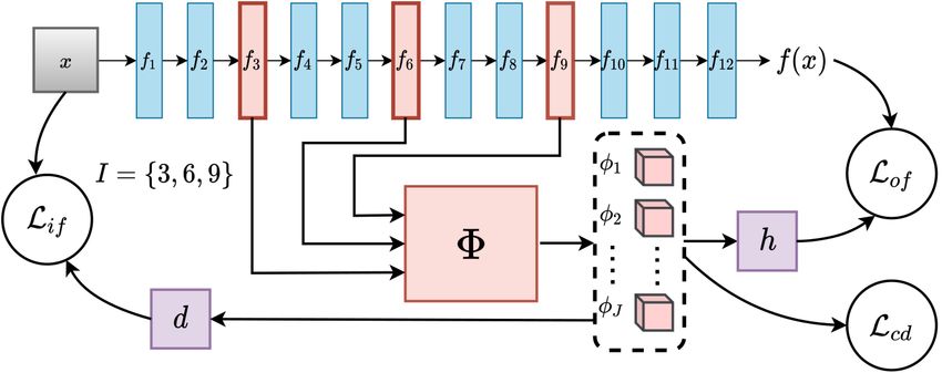
is therefore eligible. The interpreter architecture which can    mentation and clustering. ConceptSHAP (Yeh et al. 2019)
be considered as a global proxy of the predictor function ex-    further builds by introducing the idea of “completeness” or
hibits two main features. First it takes as input the outputs    importance of concepts in this framework. Self explaining
of several hidden layers of the predictor network which en-      neural networks (SENN) (Melis and Jaakkola 2018) pre-
forces by design a closeness to the predictor network. Sec-      sented a generalized linear model. The linear structure is to
ond it relies on a decomposition of its prediction on a dic-     emphasize interpretability. However to not lose out on per-
tionary of high level attribute functions. Note that this kind   formance the coefficients are modelled as a function of in-
of generalized linear model has already been used in other       put. They are modelled using much heavier neural networks
works but neither taking the outputs of several hidden layer     compared to the features. SENN imposes a gradient-based
nor being simultaneously trained with the predictor network.     penalty to learn coefficients stably and constraints to learn
This task sharing is beneficial for both networks as we show     human understandable features.
it in experiments: the predictor network even slightly im-          The CAV-based approaches strongly differ from ours in
proves its accuracy while the interpreter network builds on      the context of the problem as they produce post-hoc in-
the relevant hidden representations learned by the predictor.    terpretations. Moreover, their candidate concepts are ex-
A key feature of this approach is to design a loss function      ternally generated, either by human-supervision, or pre-
that impose a limited number of attribute functions as well      processing algorithms, and not from the network itself. The
as conciseness and diversity among the activation of these       pre-processing steps also limit the applicability on types of
attributes for a given input. The paper is structured as fol-    problems. In case of SENN, although the coefficients are
lows. We first provide a brief overview of key features of       learnt so as to behave stably, they are still output of an unin-
related works, then we introduce the whole framework. Ex-        terpretable system. This non-interpretable modelling leads
periments conducted on two image classification datasets,        to major differences with our framework. To retain inter-
MNIST and QuickDraw, are discussed before drawing con-           pretability, we don’t model the coefficients as functions of
clusion and perspectives.                                        input but rather as a linear classifier. To not trade-off accu-
                                                                 racy we allow the classifier to be modelled as unrestrained
                     Related Works                               neural network and learn an interpreter separately. More-
                                                                 over, we build an extensive pipeline for better understanding
Interpretability as part of learning Most works for in-
                                                                 of the learnt features for both local interpretations and global
terpretability focus on producinga posteriori (or post-hoc)
                                                                 interpretations.
explanations. They often consider the model as a black-
box (Lundberg and Lee 2017; Lakkaraju, Arsov, and Bas-
tani 2020; Lakkaraju et al. 2019; Bang et al. 2019) or in the                   Our framework: FLINT
case of deep neural networks, work with gradients to gener-      We describe our framework for a multi-class classification
ate saliency maps for a given input (Simonyan, Vedaldi, and      problem with C classes. Denote X = Rd the input space
Zisserman 2013; Smilkov et al. 2017; Selvaraju et al. 2017;      and Y, the output space, the set of C one-hot encoding vec-
Montavon, Samek, and Müller 2018). There are a few works        tors of dimension C. A deep neural network with l + 1
that modify either the structure of the model (Al-Shedivat,      layers of respective dimension d1 , . . . , dl+1 is a mapping
Dubey, and Xing 2017; Angelov and Soares 2020), the              f : X → Y such that: f = fl+1 ◦ fl ◦ ... ◦ f1 where
losses (Lee et al. 2019), or both (Zhang, Nian Wu, and Zhu       fk : Rdk−1 → Rdk , k = 1, ..., l + 1 is the function im-
2018; Melis and Jaakkola 2018) to incorporate interpretabil-     plemented by layer k. For any x ∈ X , the output fk (x) of
ity in the learnt model. However all these approaches offer      an intermediate layer k in f (x) is denoted xk while its di-
local interpretations, with the exception of LIME (Ribeiro,      mension is called dk . We call Fl the space of deep neural
Singh, and Guestrin 2016) and SHAP (Lundberg and Lee             networks with l + 1 layers. Alternatively, a network f in Fl
2017). Recently proposed neural additive models (Agar-           is completely identified by its generic parameter θf ∈ Θ.
wal et al. 2020) are both, globally and locally interpretable.   We describe our framework for a multi-class classification
However, their approach is currently only suitable for tabu-     problem with C = dl+1 classes. We assume that the train-
lar data, and not for more complex input like images.            ing set S = {(xi , yi )N
                                                                                        i=1 } is an i.i.d. sample from a fixed but
                                                                 unknown joint probability distribution P (X, Y ) over X ×Y.
Interpretability via human understandable features
Traditional methods for producing explanations generally
perform attribution over input features. They have been          Learning with interpretation
questioned for their robustness to simple transformations        Given the training set S, our goal is to jointly learn a pair of
to input such as constant shifts (Kindermans et al. 2017).       models, a prediction network f and an interpretation net-
This has led to interest in use of human-interpretable con-      work g. We make no special assumption on f : f can be
cepts for interpretations. TCAV (Kim et al. 2017) propose to     chosen as the state-of-the-art architecture for the multi-class
utilize human-annotated examples to represent concepts in        classification task at hand. The role of the interpreter is to
terms of activations of a pre-trained neural network, termed     provide both local and global interpretability about f in
as concept activation vector (CAV). The sensitivity of these     terms of high level attribute functions, without any loss of
concepts for prediction of each class is estimated to offer a    accuracy for f . The interpreter model g takes as inputs the
global explanation. ACE (Ghorbani et al. 2019) attempts to       outputs of several hidden layers of f to benefit from its rep-
automate the human-annotation process by super-pixel seg-        resentation learning ability. We introduce Supervised Inter-
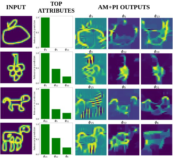
Figure 1: General scheme of FLINT. The predictor f is a deep neural network with multiple layers. The interpreter g = h ◦ Φ.
Φ takes as input intermediate outputs of f , and outputs human-interpretable attributes and h is a linear classifier

pretable Learning in the context of empirical risk minimiza-          shallow neural network, consisting only of 2-3 layers. The
tion as the following joint optimization problem:                     vector consisting of all attributes is denoted as Φ(xI ) =
                                                                      [φ1 (xI ), φ2 (xI ), ..., φj (xI )] ∈ RJ . Eventually, the inter-
            arg min Lpred (f, S) + Lint (f, g, S),
                 f,g                                                  preter network computes the following function:
where f is searched over Fl and g over the class of inter-                             ∀x ∈ X , g(x) = h ◦ Φ(xI ),
preter networks of f that we define below, Lpred (f, S) de-
notes a loss term related to prediction and Lint (f, g, S) is a       where h : RJ → RC is a linear model composed with a
loss term related to interpretability.                                ”softmax” layer. For sake of simplicity, we denote Θg =
                                                                      (θΦ , θh ) the parameters of this model. Note that other can-
                                                                      didates such as decision trees could be used instead of the
Interpretation and interpreter network Before defining
                                                                      linear classifier h.
each of the loss terms, we emphasize that we now consider
three possible uses of this pair of models. The first one is
                                                                      Imposing interpretability properties
the usual task of prediction, i.e. computing ŷ = f (x). The
second one, called here local interpretation, consists in pro-        We adopt here an axiomatic view of interpretability. To
viding insights about f (x) by extracting information from            overcome the difficulty of defining what is a human-
g(x). This should be done only if g(x) = f (x). Indeed, in            understandable attribute function, we list a number of prop-
case g(x) and f (x) disagree, this raises the questions of i)         erties desirable for an interpreter network and enforce them
trusting the prediction f (x), ii) augmenting the capacity of g       via various penalty terms additionally to the architecture
and ii) exploiting however the information brought by func-           choices. Although this kind of approach is shared by sev-
tion g. We discuss this issue in the supplements. The third           eral works in Explainable AI (Carvalho, Pereira, and Car-
use of our pair of models is to provide a global interpreta-          doso 2019), there is no consensus on these properties. We
tion of the way each class is predicted by f .                        propose here a minimal set of penalties which are relevant
   In this work, a local interpretation of f (x) is defined as        for the proposed architecture and that is sufficient to provide
a small set of high level attribute functions which are highly        relevant attribute functions.
activated when the prediction ŷ = g(x) = f (x) is com-
puted. A global interpretation is a description of each class         Fidelity to Output. Since the attributes are expected to
in terms of a small subset of high level attribute functions          provide interpretability to the network f ’s prediction, the
built from the predictor network. Moreover, a given attribute         output of the interpreter g(x) should be ”close” to the output
function captures a property of the input data that may be            f (x) for any x. This can be imposed through a cross-entropy
useful to predict different classes.                                  loss:
   Given this definition, an interpreter network g provides                                       X
a prediction by linearly combining several attribute func-                     Lof (f, g, S) = −      h(Φ(xI )T log(f (x))
tions φj , j = 1, . . . J that take as input, the outputs of sev-                                 x∈S
eral selected hidden layers (see Fig. 2). Let us call I =
{i1 , i2 , ..., iT } ⊂ {1, . . . , l + 1} the set of indexes speci-   Conciseness and Diversity. For any given sample x, we
                                                         PT
fying the layers to be accessed. We define D = t=1 dit .              wish to get a very small number of attribute functions
Typically these layers are selected from the latter layers            needed to encode relevant information about it. This prop-
of the network f . The concatenated vector of all inter-              erty of ”conciseness” should help in making the interpre-
mediate outputs for an input sample x is then denoted as              tations easier to understand. However, to encourage better
xI = fI (x) ∈ RD . The dictionary of attribute func-                  use of available attributes we also expect use of multiple at-
tions φj : RD → R+ , j = 1, ..., J is modelled by a                   tributes across many randomly selected samples.We refer to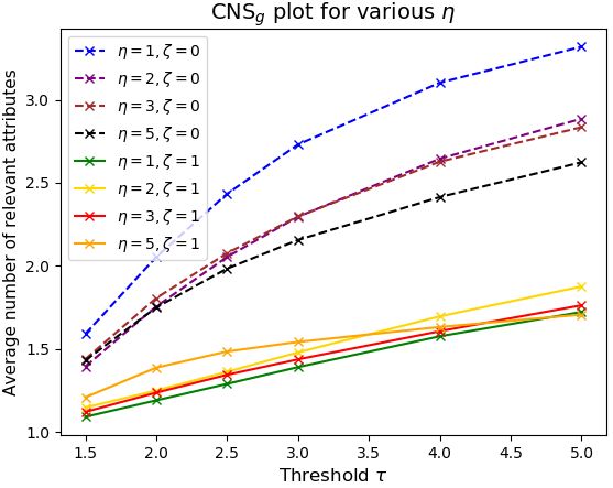
this property as diversity. To enforce these conditions we          Algorithm 1 Learning Algorithm for FLINT
rely on the notion of entropy defined for real vectors as pro-       1: Input: S & hyperparameter: β0 , γ0 , δ0 , µ0 , ζ0 , η0 &
posed for instance by (Jain et al. 2017). For P  a real-valued          number of batches B, s: size of a batch.
vector v, the entropy
                P       is defined as E(v)   = −   i pi log(pi ),    2: β = 0, γ = γ0 , δ = 0
pi = exp(vi )/( i exp(vi )).                                         3: Random initialization of parameter Θ
   Conciseness is promoted by minimizing E(Φ(xI )) and               4: for m = 0 to Nepoch − 1 do
diversity is promoted by maximizing entropy of average at-           5:     if m == 2 then
tribute vector over a mini-batch. Since entropy-based losses         6:         β = β0 , δ = δ 0 , η = η 0 , ζ = 0  . No entropy
have an inherent normalization, they do not constrain the            7:     if m == 3 then
magnitude of the attributes. This often leads to poor opti-          8:         µ = µ0 , ζ = ζ0
mization. Thus, we also minimize the `1 norm kΦ(xI )k1 to
avoid it. Note that `1 -regularization is a common tool to en-       9:     for b = 1 to B do
courage sparsity and thus conciseness, however we show in           10:         Pick up a mini-batch of size s
the experiments that entropy provides a more effective way.         11:         Compute Lpred , Lof , Lif , Lcd for mini-batch
                                                                    12:         L = Lpred + βLof + γLif + δLcd
                              1 X                                   13:         θf , θΦ , θh , θd ← Backprop(L)
                     Φ̄S =           Φ(xI )
                             |S|                                    14: return Θ
                                 x∈S
                h              X              i X
Lcd (Φ, S) = ζ −µE(Φ̄S )+          E(Φ(xI )) +       ηkΦ(xI )k1
                              x∈S                x∈S

Fidelity to Input. To encourage encoding of high-level
meaningful patterns, Φ(xI ) should encode relevant informa-
tion about the input x. Following SENN (Melis and Jaakkola
2018), we impose this using a decoder network d : RD → X
that takes as input the set of attributes Φ(xI ) and recon-
structs x.
                              X
           Lif (d, Φ, f, S) =    (d(Φ(xI )) − x)2                       Figure 2: Flow for generating global interpretations
                               x∈S

Learning Algorithm                                                  in selecting the prominently activating attributes and class-
Given the proposed loss terms, the loss for interpretability        attribute pairs commonly occurring in interpretations. We
writes as follows:                                                  propose use of multiple tools to gain understanding about
                                                                    patterns detected by attributes in the extracted pairs.
Lint (f, Φ, h, d, S) =βLof (f, Φ, h, S) + γLif (Φ, h, d, S)
                      + δLcd (Φ, S)                                 Selecting relevant class-attribute pairs For a sample x
                                                                    with predicted class ĉ (by the interpreter, h(Φ(xI ))), we
For Lpred , cross-entropy loss can be used as well. Regular-        define the total contribution of attribute j as αj,ĉ,x =
ization can also be performed through different mechanisms.         φj (xI ).wj,ĉ , where wj,ĉ are weights of linear classifier h.
   Let us denote Θ = (θf , θd , θΦ , θh ) the parameters of these   The importance of attribute j, for predicting class ĉ, for
                                                                                                   α
networks. Learning the parametric models f , Φ, h and d             sample x is, rj,ĉ,x = maxij,ĉ,x|αi,ĉ,x | . To estimate rj,c for a
boils down to learn their parameter. In practice, introducing       given class-attribute pair (j, c), we compute mean of rj,ĉ,x
all the losses at once often leads to very poor optimization.
Thus for both the datasets we follow the procedure described        P samples x where predicted class ĉ = c. That is, rj,c =
                                                                    for
                                                                       {x∈Srnd |ĉ=c} rj,ĉ,x (Srnd is random subset of the train-
in algorithm 1. We train the networks with Lpred , Lif for          ing set). To select relevant class-attribute pairs, we simply
the first two epochs and gain a reasonable level of accuracy.       threshold rj,c for each (j, c). For each such selected pair we
From the third epoch we introduce Lof and `1 -regularization        analyze the attribute’s maximum activating samples (MAS)
and from the fourth epoch we introduce the entropy losses.          from the class using the tools discussed below.
Interpretation Phase                                                Analysis tools for interpretability To understand patterns
We now present how to generate a global interpretation for          encoded by any attribute on the selected MAS for a class-
f (.) or local interpretation for any x with prediction f (x).      attribute pair, we use the following tools:
                                                                    • Input attribution: This is a natural choice to understand
Global interpretability. We create a pipeline to extract              an attribute’s action for a sample. There are a variety of
class-attribute pairs important for interpretation. We statis-        algorithms that can be employed ranging from black-box
tically estimate the relative importance of an attribute φj for       local explainers to saliency maps. While these maps are
class c, denoted by rj,c . Although this could be directly done       less noisy and easily obtained, they do not enhance en-
by analyzing parameters of h, statistically estimating it helps       coded patterns and thus the underlying patterns may not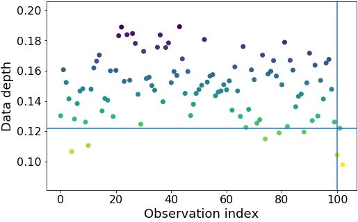
be easily distinguishable from the other parts of input.         as output of 2nd conv. layer. For the ResNet18-based net-
• Decoder: As mentioned earlier, we also train an autoen-          work, we fix I as output of the 3rd conv. block (13th conv.
  coder via a decoder d that uses the attributes as input.         layer) and middle of the 4th conv. block (15th conv. layer).
  Thus, for an attribute j and input x, we can compare the         Precise architecture details are given in the supplementary.
  reconstructed samples d(Φ(xI )) and d(Φ(xI )\j) where            Optimization All the models are trained for 12 epochs.
  Φ(xI )\j denotes attribute vector with φj (xI ) = 0, i.e.,       We use Adam (Kingma and Ba 2014) as the optimizer with
  removing the effect of attribute j.                              fixed learning rate 0.0001 and train on a single NVIDIA-
• Activation maximization and partial initialization               Tesla P100 GPU. Quantitative metrics on QuickDraw with
  (AM+PI): To focus more on enhancing a pattern detected           ResNet are averaged across 3 runs for each set of parame-
  by an attribute, synthesizing appropriate input via opti-        ters. Implementations are done using PyTorch (Paszke et al.
  mization is a common and popular idea, referred to as            2017).
  activation maximization (Mahendran and Vedaldi 2016).            Hyperparameter tuning For our experiments we set the
  In our case this optimization problem for an attribute j is:     number of attributes to J = 25, 24 for MNIST and Quick-
                                                                   Draw, respectively. For MNIST with LeNet, we set ζ =
         arg max λφ φj (xI ) − λtv TV(x) − λbo Bo(x)               1, µ = 1, η = 0.5, δ = 0.2, and for QuickDraw with ResNet,
               x
                                                                   to emphasize conciseness less and diversity more we set
  where TV(x) denotes total variation of x and Bo(x) pro-          ζ = 1, µ = 2, η = 3, δ = 0.1. We set δ = 0.1 for ex-
  motes boundedness of x in a range. For details, refer to         periments on QuickDraw and δ = 0.2 on MNIST. β = 0.1
  (Mahendran and Vedaldi 2016). Empirically, we found              is employed for QuickDraw and β = 0.5 is employed for
  that for very deep predictors, this optimization with ran-       MNIST. It’s slightly more tedious to tune γ. γ is varied be-
  dom initialization often failed (attribute failed to activate)   tween 0.8 to 20. We tune it so that the average value of Lif
  or lead to noisy results on our datasets. Thus, we initialize    on S at least halves by the last epoch of training. γ is set to
  the optimization procedure by low-intensity version of se-       0.8 for MNIST and 5.0 for QuickDraw.
  lected input sample. This makes the optimization problem
  easier with the attribute’s detected pattern weakly present      Choices for interpretation phase For a random subset
  in the input. This also allows the optimization to “fill         Srnd consisting of 1000 samples from S, we select class-
  out” the input on its own with the desired pattern of at-        attribute pairs which have rj,c > 0.1 and use gradient as at-
  tribute. For the output we obtain a map consisting of the        tribution method for LeNet based network and Guided Back-
  attribute’s detected pattern adapted to the particular input.    propagation (Springenberg et al. 2014) for ResNet based
  We treat this as our primary tool for understanding pat-         network. We fix parameters for AM+PI for all our experi-
  terns detected by an attribute.                                  ments as λφ = 2, λtv = 6, λbo = 10 and for each sample
                                                                   x to be analyzed, we analyze input for this optimization as
Local interpretability To interpret the prediction f (x)           0.1x. For optimization, we use Adam with learning rate 0.05
for any sample x one only needs to extract the importance          for 300 iterations, halving learning rate every 50 iterations.
score rj,ĉ,x (ĉ = h(Φ(xI ))argmax ), for each attribute, and
then put these with the interpretations generated for each at-     Evaluating the trained models
tribute. The tools discussed above can be used to gain more        We evaluate our model on three quantitative metrics and
precise understanding about what each attribute is detecting.      qualitatively analyze the learnt attributes. The metrics are:
One can modify ĉ and repeat the same analysis to gain un-         • Accuracy loss: To quantify effect of jointly learning the
derstanding about relevance of attributes to a different class.      interpreter on the performance of f , we also train it with
                                                                     β, γ, δ = 0 (i.e only with Lacc ) and compare the differ-
     Numerical Experiments and discussion                            ence in accuracy on test set.
Datasets and Networks                                              • Fidelity of interpreter: We quantify how well g inter-
We consider 2 datasets for experiments, MNIST (Lecun                 prets f by computing number of samples where predic-
et al. 1998) for digit recognition and subset of QuickDraw           tion of g is same as f .
dataset for sketch recognition (Ha and Eck 2018). Addi-            • Conciseness of interpretations: We propose the follow-
tional results on FashionMNIST (Xiao, Rasul, and Vollgraf            ing metric to measure the conciseness of an interpretation
2017) are available in supplementary material. In the case of        based on high-level features: For a given sample x, let the
QuickDraw, we select 10000 random images from each of                predicted class of interpreter g be ĉ and rj,ĉ,x the rele-
10 classes: ’Ant’, ’Apple’, ’Banana’, ’Carrot’, ’Cat’, ’Cow’,        vance for attribute j. We calculate conciseness for sam-
’Dog’, ’Frog’, ’Grapes’, ’Lion’. We randomly divide each             ple x, CNSg,x , as number of attributes with rj,ĉ,x greater
class into 8000 training and 2000 test images. Complete data         than a threshold 1/τ, τ > 1, i.e. CNSg,x = |{j : rj,ĉ,x >
is provided in the supplementary material.                           1/τ }|. for different thresholds τ , We compute the mean of
   Our experiments include 2 kinds of architectures for pre-         CNSg,x over test data to estimate conciseness of g, CNSg .
dictor f : (i) LeNet-based (LeCun et al. 2015) network, and
(ii) Adapted ResNet18 (He et al. 2016) (no batch normal-           Quantitative analysis
ization layers). Φ consists of 1–2 conv. layers followed by        Tab. 1 indicates the accuracy of various networks related
pooling and a FC layer. For LeNet based network, we fix I          to FLINT. Training f within FLINT does not result in any
Dataset Architecture System Accuracy (%)↑
BASE-f 99.0
MNIST LeNet FLINT-f 99.1
FLINT-g 98.4
BASE-f 85.2
QuickDraw ResNet FLINT-f 85.4
FLINT-g 85.3
Table 1: Accuracy on different datasets. BASE-f is system
trained with just accuracy loss. FLINT-f , FLINT-g denote
the predictor and interpreter trained in our framework.
Figure 3: Effect of entropy losses on conciseness of ResNet
with QuickDraw for various `1 -regularization levels.
Dataset Architecture Fidelity (%)↑
MNIST LeNet 98.8
QuickDraw ResNet 90.8
Table 2: Fidelity results for FLINT
accuracy loss on both datasets, which can be primarily at-
tributed to the design of the framework: Although all the ad-
ditional losses regularize the intermediate layers of f (their
gradient propagates to all layers before and including the
most advanced layer in I), these constraints are not directly Figure 4: Conciseness of LeNet with MNIST
placed on the layers of f (specially ones close to output),
but propagate through Φ. The flexibility in choosing the set
of intermediate layers to be used for attribute function is also tions compared to using just `1 -regularization, with the dif-
a useful possibility in this regard. ference being close to use of 1 attribute less when entropy
Tab. 2 tabulates the fidelity of g to output of f . We achieve losses are employed. On MNIST, the difference is even more
very high fidelity on MNIST, which is mainly because g ac- pronounced because of higher weight for entropy losses ζ,
cesses intermediate layers of f , but also since learning ob- weaker `1 -regularization η, and more focus on conciseness
jective encourages g to match output of f . The fidelity on during training (lower µ).
QuickDraw is also reasonably high, and the lacking 9.2%
can be explained by two main factors, see the supplemen- Qualitative analysis
tary material for illustration. First, e.g., in Apple, a very few
Global interpretation. Fig. 5 depicts part of the global
wrongly attributed by g observations are outliers. Second,
interpretability picture with various class-attribute pairs de-
a subclass (e.g. of Cat) is too small and diverse to gener-
tected for QuickDraw. We select attributes most relevant for
ate intuitive features, while f fits to it in an “unexplainable”
two of the best (Apple and Banana) and worst (Dog and
(by the features) way. Further, Tab. 3 captures the effect of
Cow) classes in terms of fidelity and me of these attributes
entropy and `1 -regularization strength on fidelity of g for
are also relevant for other classes, we include the pairs for
QuickDraw illustrating the (relatively small) price in terms
those classes as well. We show 8 out of 24 class-attribute
of fidelity to pay for the sparsity when adding entropy.
pairs in Fig. 5. For each class-attribute pair we analyse
To evaluate the conciseness of FLINT-g (also on Quick- AM+PI output for 3 MAS. Comprehensive illustration on all
Draw), we plot the average number of relevant attributes for class-attribute pairs can be found in the supplementary ma-
different values of η and ξ as a function of threshold. terial. As expected, there are attributes exclusive to a class,
The figures confirm that using the entropy-based loss is while others are relevant for multiple classes. φ3 (relevant
a more effective way of inducing conciseness of explana- for Apple only) clearly detects large circular shape, while
φ16 “draws” multiple half-strokes of a banana. Multi-class
attributes φ22 , φ5 , φ15 , though more complex, still consis-
η=1 η=2 η=3 η=5 tently detect similar patterns. This significantly contributes
ζ=0 92.7 90.4 91.2 84.2 to their understandability. φ22 shows strong activation for
blotted textures, often drawn on stomach of a cow, or as
ζ=1 91.2 90.7 90.8 82.9 dense blobs of grapes. φ15 (most relevant for Cow, Dog, &
Ant) primarily detects leg-like vertical strokes. However it
Table 3: Fidelity variation for η and ζ. All other parameters also detects strokes related to head and body, which can cor-
fixed respond to tentacles in ant and stomach for Dogs/Cows.MAS 1 AM+PI 1 MAS 2 AM+PI 2 MAS 3 AM+PI 3
Apple --
Banana--
Cow --
Grapes --
Dog --
Lion -- Figure 7: Local interpretations for test samples on Quick-
Draw. True labels for inputs are: Apple, Grapes, Dog, Cow.
Ant --
class Apple, only one attribute φ3 is important. It detects
Cow --
pattern consistent with its global interpretation. Even φ5 ,
though not relevant for prediction, detects very similar pat-
tern as in global interpretations. Attributes φ15 , φ5 , φ22 also
Dog -- demonstrate the same consistency in patterns detected as ex-
pected from global interpretation outputs.
MAS 1 GBP 1 AM+PI 1 MAS 2 GBP 2 AM+PI 2
Figure 5: Attributes learnt on QuickDraw with ResNet.
Rows correspond to a class-attribute pairs. 3 maximum acti- Apple --
vating samples are analyzed with their AM+PI outputs.
Carrot --
Figure 8: Sample attribute φ3 learnt without Lif . GBP
stands for Guided Backpropagation.
Figure 6: Sample attributes learnt on MNIST with LeNet. Effect of autoencoder loss. Although the effect of
Each row corresponds to a class-attribute pair. Three MAS Lof , Lcd can be objectively assessed to some extent, the ef-
are analyzed with their AM+PI outputs. fect of Lif can only be seen subjectively. If the model is
trained with γ = 0, the attributes still demonstrate high
overlap, nice conciseness. However, it becomes much harder
Likewise we show sample results of global interpretability to understand patterns encoded by them. For majority of
for MNIST in Fig. 6. Complete sets of figures are in the sup- attributes, MAS and the outputs of the analysis tools do
plementary. For MNIST, most attributes are class-exclusive. not show any consistency of detected pattern. One such at-
This makes them straightforward to understand. An interest- tribute, φ3 , is depicted in Fig. 8. It is relevant for both Ap-
ing observation about the learnt attributes is that for classes ple and Carrot, but it’s hard to pin down a common pattern
with multiple relevant attributes, like class ‘1’, each attribute among all 4 images. Moreover, AM+PI fails to optimize on
activates to specific types of samples for that class. E.g. φ19 3 out of 4 images. We provide figures for other attributes
detects 1’s with diagonal strokes and φ15 detects 1’s with in the supplementary material. Such attributes are present
vertical strokes. This again contributes to the understand- even for the model trained with autoencoder, but are very
ability of the attributes. This is less observed for attributes few. We thus believe that autoencoder loss enforces a consis-
learnt for QuickDraw with ResNet, most likely because of tency in detected patterns for attributes. It does not necessar-
variety (and complexity) of samples. ily enforce semantic meaningfulness in attributes, however
it’s still beneficial for improving their understandability.
Local interpretation. Fig. 7 displays the local interpreta-
tions generated for test samples of QuickDraw. f and g both Conclusion
predict the true class in all the cases. We show the top 3 FLINT is a novel framework for learning a predictor net-
relevant attributes to the prediction and their corresponding work and its interpreter network with dedicated losses. A po-
AM+PI images for QuickDraw. For the first sample, from tential attractive use of our framework consists in retainingonly the interpreter model as the final prediction tool. Fur- Kim, B.; Wattenberg, M.; Gilmer, J.; Cai, C.; Wexler, J.; Vie-
ther works concern the investigation of this direction and the gas, F.; and Sayres, R. 2017. Interpretability beyond feature
enforcement of additional constraints on attribute functions attribution: Quantitative testing with concept activation vec-
to encourage invariance and geometrical properties. Even- tors (tcav). arXiv preprint arXiv:1711.11279 .
tually nothing prevents to extend to other tasks in Machine Kindermans, P.-J.; Hooker, S.; Adebayo, J.; Alber, M.;
Learning or other data than images. Schütt, K. T.; Dähne, S.; Erhan, D.; and Kim, B. 2017. The
(Un)reliability of saliency methods.
References
Kingma, D. P.; and Ba, J. 2014. Adam: A method for
Agarwal, R.; Frosst, N.; Zhang, X.; Caruana, R.; and Hin- stochastic optimization. arXiv preprint arXiv:1412.6980 .
ton, G. 2020. Neural additive models: Interpretable machine
learning with neural nets. arXiv preprint arXiv:2004.13912 Lakkaraju, H.; Arsov, N.; and Bastani, O. 2020. Robust and
. Stable Black Box Explanations. In Proceedings of the Inter-
national Conference on Machine Learning (ICML).
Al-Shedivat, M.; Dubey, A.; and Xing, E. 2017. Contextual
explanation networks. arXiv preprint arXiv:1705.10301 . Lakkaraju, H.; Kamar, E.; Caruana, R.; and Leskovec, J.
2019. Faithful and customizable explanations of black box
Angelov, P.; and Soares, E. 2020. Towards explainable deep
models. In Proceedings of the 2019 AAAI/ACM Conference
neural networks (xDNN). Neural Networks 130: 185–194.
on AI, Ethics, and Society, 131–138.
Bang, S.; Xie, P.; Wu, W.; and Xing, E. 2019. Explaining
a black-box using Deep Variational Information Bottleneck Lecun, Y.; Bottou, L.; Bengio, Y.; and Haffner, P. 1998.
Approach. arXiv preprint arXiv:1902.06918 . Gradient-based learning applied to document recognition.
Proceedings of the IEEE 86(11): 2278–2324.
Barredo Arrieta, A.; Dı́az-Rodrı́guez, N.; Del Ser, J.; Ben-
netot, A.; Tabik, S.; Barbado, A.; Garcia, S.; Gil-Lopez, LeCun, Y.; et al. 2015. LeNet-5, convolutional neural net-
S.; Molina, D.; Benjamins, R.; Chatila, R.; and Herrera, F. works. URL: http://yann. lecun. com/exdb/lenet 20(5): 14.
2020. Explainable Artificial Intelligence (XAI): Concepts, Lee, G.-H.; Jin, W.; Alvarez-Melis, D.; and Jaakkola,
taxonomies, opportunities and challenges toward responsi- T. S. 2019. Functional Transparency for Structured
ble AI. Information Fusion 58: 82 – 115. Data: a Game-Theoretic Approach. arXiv preprint
Beaudouin, V.; Bloch, I.; Bounie, D.; Clémençon, S.; arXiv:1902.09737 .
d’Alché-Buc, F.; Eagan, J.; Maxwell, W.; Mozharovskyi, Lundberg, S. M.; and Lee, S.-I. 2017. A unified approach
P.; and Parekh, J. 2020. Flexible and Context-Specific to interpreting model predictions. In Advances in Neural
AI Explainability: A Multidisciplinary Approach. CoRR Information Processing Systems, 4765–4774.
abs/2003.07703. Mahendran, A.; and Vedaldi, A. 2016. Visualizing deep con-
Carvalho, D. V.; Pereira, E. M.; and Cardoso, J. S. 2019. Ma- volutional neural networks using natural pre-images. Inter-
chine Learning Interpretability: A Survey on Methods and national Journal of Computer Vision 120(3): 233–255.
Metrics. Electronics 8(8). Melis, D. A.; and Jaakkola, T. 2018. Towards robust in-
Doshi-Velez, F.; and Kim, B. 2017. Interpretable Machine terpretability with self-explaining neural networks. In Ad-
Learning. In Proceedings of the Thirty-fourth International vances in Neural Information Processing Systems, 7775–
Conference on Machine Learning. 7784.
Dubois, D.; and Prade, H. 2014. Possibilistic Logic-An Montavon, G.; Samek, W.; and Müller, K.-R. 2018. Methods
Overview. Computational logic 9. for interpreting and understanding deep neural networks.
Ghorbani, A.; Wexler, J.; Zou, J. Y.; and Kim, B. 2019. To- Digital Signal Processing 73: 1–15.
wards automatic concept-based explanations. In Advances Mosler, K. 2013. Depth Statistics. In Becker, C.; Fried,
in Neural Information Processing Systems, 9277–9286. R.; and Kuhnt, S., eds., Robustness and Complex Data
Guidotti, R.; Monreale, A.; Giannotti, F.; Pedreschi, D.; Structures: Festschrift in Honour of Ursula Gather, 17–34.
Ruggieri, S.; and Turini, F. 2019. Factual and Counterfac- Springer. Berlin.
tual Explanations for Black Box Decision Making. IEEE Paszke, A.; Gross, S.; Chintala, S.; Chanan, G.; Yang, E.;
Intelligent Systems . DeVito, Z.; Lin, Z.; Desmaison, A.; Antiga, L.; and Lerer,
Ha, D.; and Eck, D. 2018. A Neural Representation of A. 2017. Automatic differentiation in pytorch .
Sketch Drawings. In International Conference on Learning Ribeiro, M. T.; Singh, S.; and Guestrin, C. 2016. Why
Representations. should i trust you?: Explaining the predictions of any classi-
He, K.; Zhang, X.; Ren, S.; and Sun, J. 2016. Identity map- fier. In Proceedings of the 22nd ACM SIGKDD international
pings in deep residual networks. In European conference on conference on knowledge discovery and data mining, 1135–
computer vision, 630–645. Springer. 1144. ACM.
Jain, H.; Zepeda, J.; Pérez, P.; and Gribonval, R. 2017. Samek, W.; Montavon, G.; Vedaldi, A.; Hansen, L. K.; and
Subic: A supervised, structured binary code for image Müller, K., eds. 2019. Explainable AI: Interpreting, Ex-
search. In Proceedings of the IEEE International Confer- plaining and Visualizing Deep Learning, volume 11700 of
ence on Computer Vision, 833–842. Lecture Notes in Computer Science. Springer.Selvaraju, R. R.; Cogswell, M.; Das, A.; Vedantam, R.; Parikh, D.; and Batra, D. 2017. Grad-cam: Visual explana- tions from deep networks via gradient-based localization. In Proceedings of the IEEE International Conference on Com- puter Vision, 618–626. Simonyan, K.; Vedaldi, A.; and Zisserman, A. 2013. Deep inside convolutional networks: Visualising image classification models and saliency maps. arXiv preprint arXiv:1312.6034 . Smilkov, D.; Thorat, N.; Kim, B.; Viégas, F.; and Watten- berg, M. 2017. Smoothgrad: removing noise by adding noise. arXiv preprint arXiv:1706.03825 . Springenberg, J. T.; Dosovitskiy, A.; Brox, T.; and Ried- miller, M. 2014. Striving for simplicity: The all convolu- tional net. arXiv preprint arXiv:1412.6806 . Xiao, H.; Rasul, K.; and Vollgraf, R. 2017. Fashion-mnist: a novel image dataset for benchmarking machine learning algorithms. arXiv preprint arXiv:1708.07747 . Yeh, C.-K.; Kim, B.; Arik, S. O.; Li, C.-L.; Ravikumar, P.; and Pfister, T. 2019. On concept-based explanations in deep neural networks. arXiv preprint arXiv:1910.07969 . Zhang, Q.; Nian Wu, Y.; and Zhu, S.-C. 2018. Interpretable convolutional neural networks. In Proceedings of the IEEE Conference on Computer Vision and Pattern Recognition, 8827–8836. Zuo, Y.; and Serfling, R. 2000. General notions of statistical depth function. The Annals of Statistics 28(2): 461–482.
Supplementary material                              once it becomes large enough so that Lif , Lof are optimized
Architecture of ResNet, LeNet                                      well. The upper threshold of choosing J is subjective and
                                                                   highly affected by how many attributes the user can keep a
Figs. 9 and 10 depict the architectures used for experiments       tab on or what fidelity user considers reasonable enough. It
with predictor architecture based on LeNet (LeCun et al.           is possible that due to enforcement of conciseness, even for
2015) (on MNIST) and ResNet18 (on QuickDraw) (He et al.            high value of J, only a small subset of attributes are relevant
2016) respectively.                                                for interpretations. Nevertheless, for high J value, there is a
                                                                   risk of ending up with too many attributes or class-attribute
Experiments for number of attributes J                             pairs to analyze.
Effect of J We study the effect of choosing small values              It is important to notice that it is possible to select J from
for number of attributes J (keeping all other hyperparame-         the training set only by suing a cross-validation strategy. In
ters same). Tab. 4 tabulates the values of input fidelity loss     practise, it seems reasonable to agree on smallest value of
Lif , output fidelity loss Lof on the training data by the end     J for which the increase of the cross-validation fidelity es-
of training for MNIST and the fidelity of g to f on MNIST          timate drops dramatically, since further increase of J would
test data for different J values. Tab. 5 tabulates same val-       generate less understandable attributes with very little gain
ues for QuickDraw. The two tables clearly show that using          in fidelity.
small J can harm the autoencoder and the fidelity of inter-
preter. Moreover, the system packs more information in each        Disagreement analysis
attribute and this makes it hard to understand them, specially     In this part, we analyse in detail the “disagreement” between
for very small J. This is illustrated in Figs. 11 and 12, which    the predictor f and the interpreter g.
depict part of global interpretations generated on MNIST              First, it is important to notice that achieved by the pro-
for J = 4 (all the parameters take default values). Fig. 11        posed FLINT architecture fidelity of 98.9% on MNIST and
shows global class-attribute relevances and Fig. 12 shows          90.8% on QuickDraw is very reasonable compared to typ-
generated interpretation for a sample attribute φ2 . It can be     ical values reported in the literature. The disagreement be-
clearly seen that the attributes start encoding patterns for too   tween f and g is then close to 1.1% and 9.2%, respectively.
many classes (high number of bright spots). This also causes       To the best of our knowledge, the highest reported fidelity
their AM+PI outputs to be muddled with two many patterns.          for an explanation method on MNIST is 96.7% in the work
This adds a lot of difficulty in understandability of these at-    of (Bang et al. 2019), which is 3 times more disagreement
tributes.                                                          than FLINT. Recent methods for global interpretations (e.g.
                                                                   Lakkaraju et al. 2019) or robust local interpretations (e.g.
How to choose the number of attributes Assuming a
                                                                   Lakkaraju, Arsov, and Bastani 2020) report fidelity around
suitable architecture for decoder d, simply tracking Lif , Lof
                                                                   80% for tabular datasets. The above systems and disagree-
on training data can help rule out very small values of J as
                                                                   ment rates, as well as further interpretability frameworks
they result in poorly trained decoder and relatively poor fi-
                                                                   are obviously not comparable with FLINT since they cru-
delity of g. One can also qualitatively analyze the generated
                                                                   cially differ either while reporting results on different data
explanations from the training data to tune J to a certain ex-
                                                                   or from a systemic viewpoint on one of the following axes:
tent. Too small values of J can result in attributes encoding
                                                                   (i) treating the model as a black-box, (ii) scope of interpre-
patterns for too many classes, which affects negatively their
                                                                   tation (i.e., local vs. global), (iii) means of interpretation
understandability. It is more tricky and subjective to tune J
                                                                   (human-understandable features), (iv) having interpretabil-
                                                                   ity as a part of learning objective. Nevertheless, our results
                                                                   emphasize that FLINT disagreement numbers are reason-
             Lif (train)   Lof (train)    Fidelity (test) (%)      ably low.
  J =4         0.058          0.57               87.4                 Second, it is important to analyze in detail the type and
  J =8         0.053           0.23              97.5              the reason of disagreement between f and g, especially for
                                                                   QuickDraw data. Thus, for the ’Apple’ class, the only three
  J = 25       0.029           0.16              98.8              disagreement samples for which f delivers correct predic-
                                                                   tion (plotted in Fig. 13) are not resembling apples at all. We
Table 4: Effect of J on losses and fidelity for MNIST with         propose an original analysis approach that consists in calcu-
LeNet.                                                             lating a robust centrality measure—the projection depth—
                                                                   of these three samples as well as of another 100 training
             Lif (train)   Lof (train)    Fidelity (test) (%)      samples w.r.t. the 8000 training ’Apple’ samples, plotted in
                                                                   Fig. 14. To that purpose, we use the notion of projection
  J =4         0.094          2.08               19.5              depth (Zuo and Serfling 2000) (see also (Mosler 2013)) for
  J =8         0.079           1.48              57.6              a sample x ∈ Rd w.r.t. a dataset X which is defined as fol-
                                                                   lows:
  J = 24       0.069           0.34              90.8                                                                     !−1
                                                                                                 |hp, xi − med(hp, Xi)|
                                                                     D(x|X) = 1 + sup                                           ,
Table 5: Effect of J on losses and fidelity for QuickDraw                                p∈S d−1       MAD(hp, Xi)
with ResNet.                                                                                                                   (1)
Figure 9: Architecture of networks based on LeNet (LeCun et al. 2015). Conv (a, b, c, d), TrConv (a, b, c, d) denote a convo-
lutional, transposed convolutional layer respectively with number of input maps a, number of output maps b, kernel size c × c
and stride size d. FC(a, b) denotes a fully-connected layer with number of input neurons a and output neurons b. MaxPool(a, a)
denotes window size a × a for the max operation. AvgPool(a, a) denotes the output shape a × a for each map
with h·, ·i denoting scalar product (and thus hp, Xi being a by attributes across samples in a single pair, and even across
vector of projection of X on p) and med and MAD being the different pairs (for the same attribute). It is also notable that
univariate median and the median absolute deviation form there are some attributes whose patterns are harder to under-
the median. Fig. 14 confirms the visual impression that these stand (φ1 , φ2 in figure 16) however they rarely occur when
3 disagreement samples are outliers (since their depth in the training with autoencoder.
training class is low).
For a given sample with disagreement, if the class pre- Using decoder and input attribution Although we con-
dicted by f is among the top predicted classes of g, the dis- sider AM+PI as the primary tool for analyzing patterns en-
agreement is acceptable to some extent as the attributes can coded by attributes (for MAS of each class-attribute), other
still potentially interpret the prediction of f . The worse kind tools like input attribution and decoder d can also be helpful
of samples for disagreement are the ones where predicted in deeper understanding of the attributes. We illustrate the
by f class is not among the top g predicted classes, and even use of these tools for certain example class-attribute pairs
worse are where, in addition to this, f predicts the true la- on QuickDraw in Fig. 18 and 19. Note that as discussed in
bel. We thus compute the top-k accuracy (for k = 2, 3, 4) the main paper, these tools are not guaranteed to be always
on QuickDraw with ResNet, which for the default parame- insightful, but their use can help in some cases.
ters described in the main paper, achieves a top-2 accuracy Fig. 18 depicts example class-attribute pairs where de-
of 94.7%, top-3 accuracy 96.9%, and top-4 accuracy 98.2%. coder d contributes in understanding of attributes. The with
E.g., there are only 141 (i.e. only 0.7%) of cases where the φj column denotes the reconstructed sample d(Φ(xI )) for
correctly predicted by f class is not in top-3 predicted by g the maximum activating sample x under consideration. The
classes. Fig. 15 depicts 26 such cases for ’Cat’ class to il- without φj column is the reconstructed sample d(Φ(xI )\j)
lustrate their logical dissimilarity. Being a complex model, with the effect of attribute φj removed for the sample under
the ResNet-based predictor f still manages to learn to dis- consideration (φj (xI ) = 0). For eg. φ1 , φ23 , strongly rele-
tinguish these cases (while g does not), but in a way g does vant for Cat class, detect similar patterns, primarily related
not manage at all to explain. Eventually, exploiting disagree- to the face and ears of a cat. The decoder images suggest
ment of f and g could be used as a means to measure trust- that φ1 very likely is more responsible for detecting the left
worthiness. Deepening this issue is left for future works. ear of cat and φ23 , the right ear. Similarly analyzing decoder
images for φ22 in the third row reveals that it is likely has
a preference for detecting heads present towards the right
Additional Results for Global Interpretations
side of the image. This is certainly not the primary pattern it
We depict the interpretation of other attributes on Quick- detects as it mainly detects blotted textures, but it certainly
Draw & MNIST in Fig. 16 and Fig. 17 respectively. For carries information about head location to the decoder.
each class-attribute pair, following the main paper, we se- Fig. 19 depicts example class-attribute pairs where input
lect 3 maximum activating samples, analyze it using AM+PI attribution contributes in understanding of attributes. We use
output. One can observe the consistency of patterns detected Guided Backpropagation (Springenberg et al. 2014) (GBP)Figure 10: Architecture of networks for experiments on QuickDraw with network based on ResNet (He et al. 2016). Conv (a,
b, c, d), TrConv (a, b, c, d) denote a convolutional, transposed convolutional layer respectively with number of input maps a,
number of output maps b, kernel size c × c and stride size d. FC(a, b) denotes a fully-connected layer with number of input
neurons a and output neurons b. AvgPool(a, a) denotes the output shape a × a for each map. Notation for CBlock is explained
in the figure.
MAS 1 AM+PI 1 MAS 2 AM+PI 2 MAS 3 AM+PI 3
Three --
Five --
Seven --
Figure 12: Interpretation for attribute φ2 for model learn on
MNIST with J = 4.
Figure 11: Global class attribute relevances for model with
J = 4 on MNIST. regions of the map correspond to curves similar to dog ears.
Fig. 20 shows the global class-attribute relevances (for all
pairs) for QuickDraw & MNIST. Fig 21 shows relevances
as input attribution method for ResNet on QuickDraw. It of attributes for 80 random test samples, on QuickDraw and
mainly assists in adding more support to our previously de- MNIST. One can notice the similarities in the aggregated
veloped understanding of attributes. For example, analyzing global relevances in fig. 20 and relevances for test samples
φ5 (relevant for Dog, Lion) based on AM+PI outputs sug- in fig. 21. This consistency in action of attributes for test
gested that it mainly detects curves similar to dog ears. The samples further supports our understanding from the gener-
GBP output support this understanding as the most salient ated interpretations.Figure 13: The three ’Apple’ class samples classified cor-
rectly by f but not by g. Figure 15: 26 samples from ’Cat’ class which are not in top3
f -predicted classes.
MAS 1 AM+PI 1 MAS 2 AM+PI 2 MAS 3 AM+PI 3
Cat --
Frog --
Grapes --
Lion --
Figure 14: Projection data depth calculated with (1) w.r.t. Cow --
the 8000 ’Apple’ training sample for 100 ’Apple’ test sam-
ples and for the three (observation indices 101–103) ’Apple’
class samples classified correctly by f but not by g. Ant --
Global interpretation for Non-AE model Fig. 22 shows Frog --
4 attributes and the corresponding class-attribute pairs for
model trained without autoencoder on QuickDraw with
ResNet, that is γ = 0. As remarked in the main paper, Grapes --
the patterns encoded attributes learnt for this model do not
show much consistency for different samples. This is the
Carrot --
case for most attributes in the figure (class-attribute pairs for
φ10 , φ12 , φ22 , 3rd row onwards).
Cat --
Additional results on FashionMNIST
We compute additional results on FashionMNIST (Xiao, Ra-
sul, and Vollgraf 2017). We use the same architecture for Cow --
the networks and hyperparameters as for MNIST (based on
LeNet). The accuracies and fidelity values are reported in
Tabs. 6 and 7. Global interpretations of sample attributes is Grapes --
depicted in Fig. 23.
Dog --
Cat --
Dataset Architecture System Accuracy (%)↑ Figure 16: Global overview of learnt attributes on Quick-
Draw with ResNet (does not contain attributes in main pa-
BASE-f 90.3
per). Each row is composed of analysis of single class-
FashionMNIST LeNet FLINT-f 90.6
attribute pair with 3 MAS and their AM+PI outputs.
FLINT-g 87.5
Table 6: Accuracies on FashionMNIST.MAS 1 AM+PI 1 MAS 2 AM+PI 2 MAS 3 AM+PI 3
Six --
Five --
Zero --
Eight --
Five --
Four --
Seven --
Three --
Two --
Six --
Five --
Three --
Nine --
Figure 17: Global overview of attributes learnt on MNIST
with LeNet. Each row is composed of analysis of single
class-attribute pair with 3 MAS and their AM+PI outputs.
Dataset Architecture Fidelity (%)
FashionMNIST LeNet 91.5
Table 7: Fidelity result for FashionMNIST test setDecoder Images Decoder Images Decoder Images
MAS 1 GBP 1 with without AM+PI MAS 2 GBP 2 with without AM+PI MAS 3 GBP with without AM+PI
Cat --
Cat --
Cow --
Figure 18: Examples of class-attribute pairs on QuickDraw, where decoder assists in understanding of patterns for the attribute.
Decoder Images Decoder Images Decoder Images
MAS 1 GBP 1 with without AM+PI MAS 2 GBP 2 with without AM+PI MAS 3 GBP with without AM+PI
Dog --
Lion --
Figure 19: Examples of class-attribute pairs on QuickDraw, where input attribution (GBP) assists in understanding of encoded
patterns for the attribute. GBP stands for Guided Backpropagation.
(a) Relevances for all class-attribute pairs on QuickDraw (b) Relevances for all class-attribute pairs on MNIST
Figure 20: Global class-attribute relevances for QuickDraw & MNIST. On x-axis is the class labels and on y-axis is the attribute
numbers.(a) Relevances for 80 random test samples on QuickDraw shuffled according to classes. x-axis denotes the true class label for the sample.
0: Ant, 1: Apple, 2: Banana, 3: Carrot, 4: Cat, 5: Cow, 6: Dog, 7: Frog, 8: Grapes, 9: Lion
(b) Relevances for 80 random test samples on MNIST shuffled according to classes. x-axis denotes the true class label for the sample.
Figure 21: Local relevances of the attributes for a selection of test samples.MAS 1 AM+PI 1 MAS 2 AM+PI 2 MAS 3 AM+PI 3
Sandal --
MAS 1 GBP 1 AM+PI 1 MAS 2 GBP 2 AM+PI 2
Sneaker --
Apple --
T-shirt/Top --
Frog --
Shirt --
Ant --
Sandal --
Banana --
Bag --
Cat -- Dress --
Frog -- Trouser --
Banana -- Pullover --
Grapes -- Coat --
Figure 22: Global overview of sample attributes learnt on Shirt --
QuickDraw with ResNet but without any autoencoder (γ =
0). GBP stands for Guided Backpropagation.
Figure 23: Global overview of sample attributes learnt on
FashionMNIST with LeNet. Each row is composed of anal-
ysis of single class-attribute pair with 3 MAS and their
AM+PI outputsYou can also read