A Local and Time Resolution of the COVID-19 Propagation-A Two-Dimensional Approach for Germany Including Diffusion Phenomena to Describe the ...
←
→
Page content transcription
If your browser does not render page correctly, please read the page content below
Article
A Local and Time Resolution of the COVID-19 Propagation—A
Two-Dimensional Approach for Germany Including Diffusion
Phenomena to Describe the Spatial Spread of the
COVID-19 Pandemic
Günter Bärwolff

                                          Department of Mathematics, Technische Universität Berlin, D-10623 Berlin, Germany;
                                          baerwolf@math.tu-berlin.de

                                          Abstract: The understanding of factors that affect the dissemination of a viral infection is fundamental
                                          to help combat it. For instance, during the COVID-19 pandemic that changed the lives of people
                                          all over the world, one observes regions with different incidences of cases. One can speculate that
                                          population density might be one of the variables that affect the incidence of cases. In populous areas,
                                          such as big cities or congested urban areas, higher COVID-19 incidences could be observed than
                                          in rural regions. It is natural to think that if population density is such an important factor, then a
                                          gradient or difference in population density might lead to a diffusion process that will proceed until
                                          equilibrium is reached. The aim of this paper consists of the inclusion of a diffusion concept into the
                                          COVID-19 modeling. With this concept, one covers a gradient-driven transfer of the infection next to

                                   epidemic growth models (SIR-type models). This is discussed for a certain period of the German
                                          situation based on the quite different incidence data for the different federal states of Germany. With
Citation: Bärwolff, G. A Local and
Time Resolution of the COVID-19
                                          this ansatz, some phenomena of the actual development of the pandemic are found to be confirmed.
Propagation—A Two-Dimensional             The model provides a possibility to investigate certain scenarios, such as border-crossings or local
Approach for Germany Including            spreading events, and their influence on the COVID-19 propagation. The resulting information can
Diffusion Phenomena to Describe the       be a basis for the decisions of politicians and medical persons in charge of managing a pandemic.
Spatial Spread of the COVID-19
Pandemic. Physics 2021, 3, 536–548.       Keywords: COVID-19 model; 2-dimensional diffusion; long/small-scale transmission
https://doi.org/10.3390/physics3030033

Academic Editors: Reinhard
Schlickeiser and Martin Kröger            1. Introduction
                                               The curves of infected, susceptible and recovered people, which can be found in every
Received: 10 May 2021
Accepted: 14 June 2021
                                          newspaper, describe the global pandemic behavior of the whole country, e.g., Italy, France
Published: 7 July 2021
                                          or Germany. The mathematical modeling of COVID-19 with susceptible-infected-recovered
                                          (SIR) type models [1–7] leads to averaged results and does not take into account unequal
Publisher’s Note: MDPI stays neutral
                                          population numbers or population densities.
with regard to jurisdictional claims in
                                               However, it is known that these issues play an important role in the local pandemic
published maps and institutional affil-   evolution (see, e.g., [8]). Based on the local-dependent density of people and a diffusion
iations.                                  model, the COVID-19 propagation is considered here to be resolved in a finer manner.
                                               The structure of this paper is organized as follows. In Section 2, the diffusion concept
                                          is explained. The German database is analyzed and discussed in Section 3. The numerical
                                          solution method of the initial boundary value diffusion problem is described in Section 4,
                                          and the qualitative properties of the diffusion model simulation results are given results in
Copyright: © 2020 by the author.
Licensee MDPI, Basel, Switzerland.
                                          Section 5. In Section 6, local transmission effects are modeled, joined onto the diffusion
This article is an open access article
                                          model, and then, applied to the German pandemic situation in April/May 2021. Section 7
distributed under the terms and           concludes the studies with a summary of main results.
conditions of the Creative Commons
Attribution (CC BY) license (https://
                                          2. The Mathematical Diffusion Model
creativecommons.org/licenses/by/              What is a good choice of quantity to describe the COVID-19 spread? The World Health
4.0/).                                    Organization (WHO) and national health institutions measure the COVID-19 spread with

Physics 2021, 3, 536–548. https://doi.org/10.3390/physics3030033                                           https://www.mdpi.com/journal/physics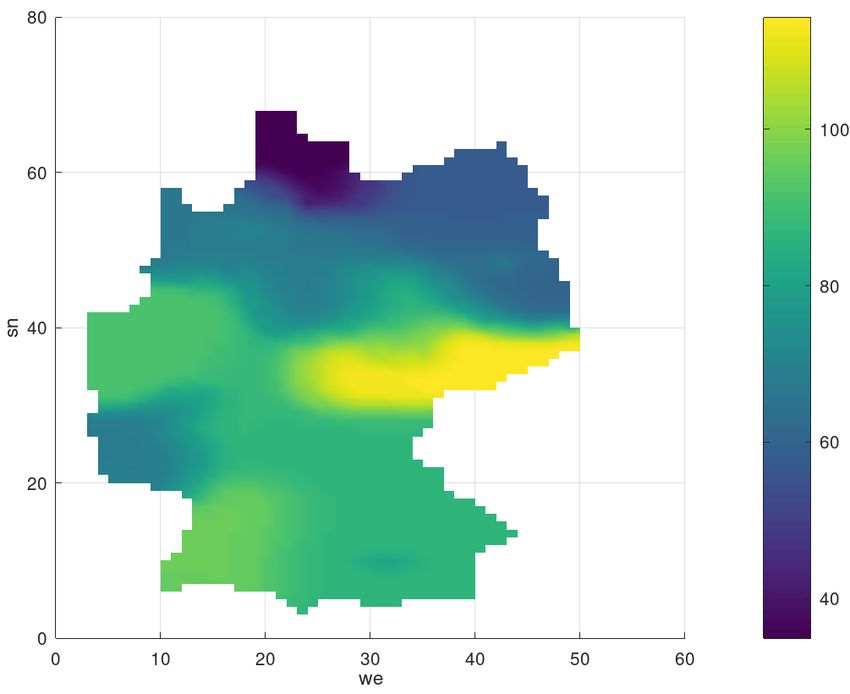
Physics 2021, 3                                                                                               537

                  the seven-day incidence (WHO also uses the fourteen-days incidence) of people with
                  COVID-19 per 100,000 inhabitants. In Germany, it is possible to control or trace the history
                  of people with COVID-19 by local health institutions if the seven-day incidence has a value
                  less than 50. However, between the end of December 2020 and the beginning of January
                  2021, the averaged incidence was about 140 and, in some hot-spot federal states, such as
                  Saxony, it was greater than 300. At the end of March and at the beginning of April, the
                  incidences changed dramatically. However, in general, one considers a different pandemic
                  development from one federal state to another and this situation needs to be respected
                  with the consideration of diffusion phenomena.
                        If the social and economical life should be sustained, there are several possibilities of
                  transmitting the COVID-19 virus. Among others, the following ones to be mentioned:
                  •    commuters and employers on the way to their office or to their position of employment,
                       especially medical and nursing staff;
                  •    pupils and teachers in schools and on the way to school;
                  •    people buying everyday necessities using shopping centers;
                  •    postmen, suppliers and deliverers.
                        All of these activities take place during so-called lock-downs in Germany, with the
                  result of an ongoing propagation of the pandemic. Furthermore, the unavailable center of
                  power in the decentralized federal states of Germany often leads to solo efforts of some
                  federal states.
                        From authoritarian countries, such as China or Singapore, with quite a different
                  civilization and cultural traditions than those in Germany, it is known that the virus
                  propagation could be stopped with very rigorous measures such as the strict prohibition of
                  social and economic life. Those ones mentioned-above are absolutely forbidden.
                        This is inconceivable in countries like Germany, Austria, the Netherlands or other so-
                  called democratic states with a western understanding of freedom and self-determination.
                  However, as a consequence of such a western lifestyle, they have to live with more or
                  less consecutive activity of the COVID-19 pandemic. This is the reason for the following
                  trial: to describe one aspect of the pandemic by a diffusion model. In connection with
                  the pandemic, diffusion has been discussed, e.g., in [9–11]. The diffusion being a central
                  process in many biological, social, chemical and physical systems is considered in [12,13].
                  A similar model but in another context has been discussed in [14].
                        Within the diffusion concept considered here, the seven-day incidence, denoted by
                  s, serves as the quantity that is influenced by its gradients between different levels of
                  incidence in the federal states of Germany. The mathematical model of diffusion of a
                  certain quantity c is given by [15]:

                                              ∂c
                                                 = ∇ · ( D ∇c) + q           in [t0 , T ] × Ω,                (1)
                                              ∂t

                  where Ω ⊂ R2 is the region that will be investigated (for example, the national territory of
                  Germany), D is a diffusion coefficient, depending on the locality x ∈ Ω, [t0 , T ] is the time
                  interval of interest, and q is a term that describes sources or sinks.
                       Now the seven-day incidence s should be considered as such a quantity with the term
                  q that describes of possible infections.
                       In addition to Equation (1), one needs to define initial conditions for s, such as, e.g.,

                                                    s( x, t0 ) = s0 ( x ),    x ∈ Ω,                          (2)

                  and boundary conditions,

                                               αs + β∇s · ~n = γ        in [t0 , T ] × ∂Ω ,                   (3)

                  where α, β and γ are real coefficients, ∂Ω =: Γ denotes the boundary of the region Ω, and
                  ∇n s = ∇s · ~n is the directional derivative of s in the direction of the outer normal vector
Physics 2021, 3                                                                                             538

                  ~n on Γ. The choice of α = 0, β = 1 and γ = 0 leads, for example, to the homogeneous
                   Neumann boundary condition:
                                                         ∇n s = 0 ,                                 (4)
                  which means no import of s at the boundary Γ. In other words, Equation (4) describes
                  closed borders to surrounding countries outside Ω.
                       The diffusion coefficient function, D : Ω → R, is responsible for the intensity or
                  velocity of the diffusion process. From fluid or gas dynamics [16]:

                                                                 2
                                                           D=      v̄λ ,                                    (5)
                                                                 3
                  with the averaged particle velocity, v̄, and the mean free path, λ. The application of this
                  ansatz to the movement of people in certain areas requires some assumptions for v̄ and
                  λ. The discussion of the mean distance of people in a certain federal state considering
                                                                                                        √ the
                  means distances of homogeneous distributed people leads to the relation, λ = A/N,
                  with the area, A, and a number of inhabitants, N, for the relevant federal state.
                        From the physics of particle movement [16], λ = 1/(ρσ), where ρ is the density and
                  σ is the total cross-sectional area of collisions. The application of the three-dimensional
                  diffusion theory [17] to the two-dimensional area leads to σ ≈ 0.2 m, i.e., to the averaged
                  size of a person’s head. Let us assume the velocity v̄ spanning 50 to 100 km/day, which is
                  a gauge of mobility [9,10]. Another suggesting heuristic is given with the assumption of D
                  assumed to be proportional to the people density. The first ansatz, based on Equation (5),
                  was applied in the simulations with v̄ = 100 km/day. However, these approaches looks
                  to be a coarse approximation of such diffusion processes. As soon as the people densities
                  (areas and number of inhabitants) of the federal states of Germany are different, D is
                  expected to be a location-depending non-constant function. This means that the diffusion
                  phenomenon is supposed to be of a different intensity in the different federal states of
                  Germany. The data given in Table 1 define the function D. For example, one finds
                  D = 0.48875 km2 /day for Bavaria, and D = 0.64355 km2 /day for Saxony-Anhalt.
                        To note is that one can consider non-linear diffusion models with coefficient D depend-
                  ing on s, but in this paper, the diffusion coefficients are supposed to be location-dependent
                  only. Meantime, this is a generalization with respect to other diffusion models where the
                  diffusion coefficient is kept constant; see, e.g., [9].
                        If there are no sources or sinks for s, i.e., q = 0, and the borders are closed, which
                  means for the boundary condition (4), the initial boundary value problem of Equations (1),
                  (2) and (4) has the steady-state solution:
                                                           R
                                                              s0 ( x ) dx
                                                     sst = Ω R            = const.                          (6)
                                                               Ω dx

                       This is easy to be verified, and this property is a characteristic of diffusion processes
                  tending to equilibrium. It is quite complicate to model the source-sink function q in an
                  appropriate way. q depends on the behavior of the population and the health policy of
                  different federal states. Therefore, only very rough guesses can be made. It is known that
                  people in Schleswig-Holstein are exemplary with respect to the recommendations to avoid
                  infection with the COVID-19 virus which means q < 0. On the other hand, in Saxony,
                  people did not follow the indicated protocols, which means q > 0 for a long time (the
                  government of Saxony has since changed the policy leading to q < 0).
                       However, regardless of these uncertainties, one can obtain information about the
                  pandemic propagation, for example, the influence of hot-spots of high incidences (Saxony)
                  to regions with low incidences (for example, South of Brandenburg).
Physics 2021, 3 539
Table 1. Seven-day incidences of 14th January and April 26th, and corresponding people density
(per km2 ), inhabitants (per 100,000), and areas of the federal states of Germany (in km2 ).
States Jan 14th Apr 26th Density Inhabitants Area
Schleswig-Holstein 92 74 183 2904 15,804
Hamburg 115 105 2438 1847 755
Mecklenburg-West 117 139 69 1608 23,295
Pomerania
Lower Saxony 100 119 167 7994 47,710
Brandenburg 212 128 85 2522 29,654
Berlin 180 138 4090 3669 891
Bremen 84 158 1629 681 419
Saxony-Anhalt 241 180 109 2195 20,454
Thuringia 310 227 132 2133 16,202
Saxony 292 232 221 4072 18,450
Bavaria 160 179 185 13,125 70,542
Baden-Wuerttemberg 133 196 310 11,100 35,784
North Rhine-Westphalia 131 187 526 17,947 34,112
Hesse 141 180 297 6288 21,116
Saarland 160 143 385 987 2571
Rhineland-Palatinate 122 143 206 4094 19,858
Munich 156 147 4700 1540 310
3. Data of the Different Federal States of Germany
At the beginning of the year 2021 (14th of January), the Robert Koch Institut (RKI), be-
ing responsible for the daily COVID-19 data collection, published the seven-day incidence
data (of January the 14th, 2021 [8]), summarized in Table 1. The values of Table 1 are used
as initial data for the function s0 of Equation (2).
The data in Table 1 are used as a base for the determination of the diffusion coefficient
function.
4. The Numerical Solution of the Initial Boundary Value Problem
Based on the subdivision of Ω (area of Germany) into finite rectangular cells ω j , j ∈ IΩ ,
where IΩ is the index set of the finite volume cells, and Ω = ∪ j∈ IΩ ω j , Equation (1) was
spatially discretized with a finite volume method. Along with the discrete boundary
condition Equation (4), one gets a semi-discrete system continuous in time
∂s j
= ∇h · ( D ∇h s j ) + q j , j ∈ IΩ , (7)
∂t
where the h indicates the discrete version of the ∇-operator. The finite volume method is
of a spatial order two; see, e.g., [18]. The time discretization is done with an implicit Euler
scheme of order one. This allows us to work without strict restrictions for the choice of the
discrete time-step ∆t . At each time-level, one has to solve the linear-equation system,
1 n +1 1 n
s j − ∇h · ( D ∇h snj +1 ) = s + q j , j ∈ IΩ , (8)
∆t ∆t j
for n = 0, . . . , N, N = ( T − t0 )/∆t . s0j was set to the incidence s0 ( x ) for x ∈ ω j , j =
1, . . . , IΩ .
Due to the complex geometry of the region Ω with the Jacobi method, an iterative
solution method for Equation (8) of the form As = b was used. The coefficient matrix A
is irreducibly diagonal dominant, and therefore, the convergence of the Jacobi-iteration
method arises. For the discretization parameters, ∆t values in the range of 0.1 to 1 day were
chosen. The 2-dimensional spatial discretization parameters ∆ x and ∆y range 7 to 14 km.Physics 2021, 3 540
With those discretization parameters, seven to twelwe Jacobi-iterations are necessary to
comply with the criterion (Euclidian norm of the relative error),
||sn+1,i+1 − sn+1,i ||2Physics 2021, 3 541
Figure 2. Rough contour of Ω and its discretization.
For the time-behavior simulations, let us start with the case q = 0. ∆t is then set to a
half-day. Figure 3 displays the initial state. The initial state is a piece-wise constant function
with values of the seven-day incidence of the 16 federal states where Munich is considered
as a town with over a million inhabitants taken separately as it was excluded from Bavaria.
Figure 4 shows the development of the diffusion process with the change in contour
lines of s of the levels 135, 155, 175, 195, and 215 over a period of 100 days. Especially in
the border regions (Saxony—Brandenburg, Saxony—Bavaria, Saxony—Thuringia), one can
observe a transfer of incidence from the high level incidence of Saxony to the neighbored
federal states. Furthermore, the high incidence level of Berlin was transferred to the nearby
Brandenburg region. The north states with a low incidence level were only influenced by
the other states weakly. A typical smoothing and decreasing of the incidence gradients can
also be observed. The short-horizon forecast confirms the qualitative development of the
incidence in Germany. A finer resolution of the incidence propagation will be considered
below by finer modeling of the source-sink term q.
In Figure 4, the development of the seven-day incidence of a high incidence region
(Dresden) compared to a low incidence region (South Brandenburg) is shown. With the
parameters α, β and γ of the boundary condition Equation (3), it is possible to describe
several situations at the borders of the boundary Γ of Ω. The case with α = 0, β = − D and
γ 6= 0 describes a flux through the border. Such scenario is used in the following example
to describe the way home of people with COVID-19 from Austria to Bavaria.
The boundary condition at the border crossing reads:
− D ∇s · ~n = γ .
The initial state s0 the same as in the example above. γ > 0 means an “inflow” of
people with COVID-19, γ < 0 indicates a loss of people with COVID-19, while γ = 0
refers to a closed border. In Figure 5, the move of the contour lines of s for the case
γ = 250 km/day is shown.Physics 2021, 3 542
Figure 3. Contour lines of the seven-day incidence, s, at the time t = 15 days (left panel), and
t = 125 days (right panel).
Figure 4. Time–history of s of Dresden/Saxony (upper curve) and South Brandenburg (bot-
tom curve).Physics 2021, 3 543
Figure 5. Contour lines of s at t = 15 days (left panel), t = 125 days (right panel), with the
source-sink function q = 0, and the coefficient γ = 250 km/day.
At the south border of Bavaria, one can observe the increase of s caused by the flux of
s from Austria to Bavaria.
The results without a source-sink-term (q = 0) describe the qualitative trend, which
was observed in the pandemic development. To describe the whole pandemic process of
long-scale diffusion and the small-scale local virus transmission, it is necessary to consider
local epidemic spreading models, as it is done in the next Section.
6. Consideration of the Local Transmission via a SIR-Model in the Diffusion Model
The previous section demonstrates the diffusion as a long-scale process. On the other
hand, a small-scale process occurs with the direct virus transmission via epidemiological
infection. This process can be described with a SIR-model, for example.
The change of s per day can be divided into a part coming from diffusion and another
part coming from the local passing of the virus. The second issue will be modeled with the
SIR-model. The local virus transmission means, in other words, the consideration of an
SIR-model in the federal states of Germany separately. The SIR-model is defined by the
following system of equations (see, e.g., [1,19]):
dS j Ij
= −κ j S , (9)
dt Nj j
dIj Ij
= κj S − η j Ij , (10)
dt Nj j
dR j
= η j Ij , (11)
dt
where j defines the respective federal state, and S j , Ij and R j are the groups of susceptible,
infected and recovered people. Nj is the population of the respective federal state. η is the
reciprocal value of the typical time from infection to recovery (η = 1/14 ≈ 0.07). κ j is the
average number of contacts per person per time multiplied by the probability of disease
transmission for a contact between a susceptible and an infectious subject.Physics 2021, 3 544
Instead of Equations (9) and (10), one also considers the stochastic differential equa-
tions (SDEs):
S jt
dS jt = −κ j I dt − νIjt dWt (12)
N jt
Sj
dIjt = (κ j t Ijt − η Ijt ) dt + νIjt dWt (13)
N
dR jt = η Ijt dt . (14)
Here, Ijt , S jt and R jt denote stochastic processes, and Wt is a Wiener process with its main
√
characteristic, Wt − Ws ∼ N (0, t − s), t > s, and the independence of Wt and Ws for t 6= s.
With the addend νIjt dWt , one can describe random fluctuations of people with COVID-19,
for instance, unrecognized or over/under-estimated people with COVID-19. The scope of
such random effects can be controlled by the parameter ν.
The relation between the actual reproduction number, R, and κ and η is R = κ/η.
To clarify about a possible relation between actual non-pharmaceutical measures of
the government and the values of κ (or R), let us consider the development of people with
COVID-19 in the period from 18 November 2020 to 24 April 2021.
Figure 6 shows the RKI data [8] and the result of the simulation with the SIR-model.
The curve shows the implication of the drastic changes of the measures by the politicians
with a sequence of local minimums followed by local maximums. The first local minimum
seen was reached on December the 5th, the first local maximum found was on December
the 24th, the next minimum found was on 7 January 2021, and the next local maximum was
on January the 14th. In Table 2, the possible values of κ to obtain the curve of the people
with COVID-19 for the simulation with the SIR-model are shown. The possible κ-values
for the chronological periods are obtained with a simple trial-and-error method.
Figure 6. Comparison of real data [8] and simulation results.Physics 2021, 3 545
Table 2. Simulated period-depending average number of contacts per persone per time, κ, and actual
reproduction number, R, for Germany.
Period κ R
18 November 2020–23 November 2020 0.068 0.97143
24 November 2020–6 January 2021 0.92 1.3143
7 January 2021–13 January 2021 0.12 1.7143
14 January 2021–13 February 2021 0.028 0.4
14 February 2021–2 April 2021 0.092 1.3143
3 April 2021–8 April 2021 0.028 0.4
9 April 2021–15 April 2021 0.1464 2.0914
16 April 2021–24 April 2021 0.076 1.0857
The measures of the government from the end of April 2021 can be compared with
the measures of the period beginning at the 14th of January with a κ-value of 0.028. For the
propagation of the pandemic from April the 25th, this κ-value is used. Due to the fact that
the measures of the government are based on the infection control law, which are valid
from 25 April 2021, the same κ-value is used for all federal states of Germany.
In what follows, the diffusion model (1), (2), (4) coupled with the SIR-model (9)–(11)
is used.
To take into account the long-scale and small-scale processes, one considers, after
the diffusion steps with the size ∆t , the model (9)–(11) for a time-interval ∆t . This means
to solve a family of initial value problems in the interval [t p , t p + ∆t ] in every diffusion
step of Equation (8) from t p to t p + ∆t (see Algorithm 1). The initial values for Ij (t p ) are
used as the mean values of s (Table 1) of the respective federal states. The first values
of R j (t p ) (in the first diffusion step) are set to zero and the S j (t p ) values come from the
relation Nj = S j + Ij + R j . The result of the initial value problem Ij (t p + ∆t ) is converted to
s j (t p + ∆t ) and used to determine q for Equation (8) by the changing rate of s j , which means
s j (t p + ∆t ) − s j (t p )
q( x, t p + ∆t ) = , x ∈ ωj ,
∆t
during the time ∆t , caused by the process modeled with the equation system (9)–(11). In
the deterministic case (ν = 0), the Euler method is used to solve the initial value problem
per diffusion time-step (with a time-step of δt = ∆t /10). For constant coefficients κ, η
there are possibilities of finding analytic solutions of the SIR-system, which can be found
in [20,21]. However, for time-dependent coefficients, numerical methods to be used to find
a solution. If ν 6= 0 (stochastic case), the SDE system (12)–(14) is solved using the Milstein
method [22]. Here, it is important to note that the step-sizes ∆t and δt used are chosen
heuristically. Let us note that the analysis of the physics of time-scales of both the local
transmission and the diffusion process is an interesting point and should be considered
in further investigations of such combined modeling together with the parameters of the
diffusion process; see, e.g., [23].
Due to the poor informativeness of surface graphs and contour lines, the propagation
of the people with COVID-19 in Bavaria is used to compare the simulated results with
the real data of the RKI. The result of the diffusion model coupled with the stochastic SIR-
model (ν = 0.25) over the period of April 26th to May 5th is shown in Figure 7 (∆t = 1 day,
δt = ∆t /10). In addition, to the nine days where the real data are known, a forecast up to
the 16th of May 2021 is made.
For the reinterpretation (by counting back using the people densities and the area
of the federal states) of the result for the seven-day incidence, in Figure 8 the incidence
with the congruous distribution of the people with COVID-19 per square kilometer is
considered. It is obvious that the people with COVID-19 are concentrated in the congested
urban and metropolitan areas such as Munich, Hamburg, Berlin, and Ruhr.Physics 2021, 3 546
Algorithm 1 Diffusion model coupled with the SIR-model.
for j = 1, ..., M, diffusion time-steps do
Initialization: Inhabitants, density, aread data of the federal states, model parameter
for i = 0, ..., N−1, SIR time-steps per diffusion time-step do
for k = 1, ... , 17, number of federal states added by Munich do
Local transmission of the pandemic in state k, development of people with COVID-
19, integration of Equations (12)–(14)
end for
end for
Determination of the source term q using the change rate of people with COVID-19
Solution of Equation (8)
end for
Figure 7. Course of people with COVID-19 in Bavaria, from 26 April 2021 to 5 May, without diffusion
(left panel) and with diffusion (right panel).
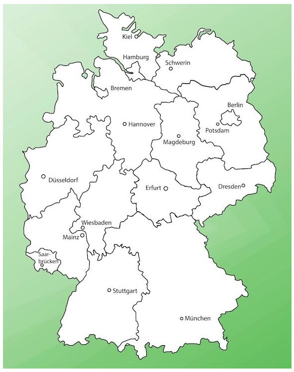
Figure 8. Forecast of the seven-day incidence, s, (left panel), and distribution of people with COVID-19 (right panel) after
20 days, for the SIR-model coupled with the diffusion concept.Physics 2021, 3 547
7. Discussion and Conclusions
The numerical simulations show an impact of diffusion effects on the propagation of
the COVID-19 pandemic. Specifically, the observed influence of high incidence regions of
Saxony and Bavaria on neighbored regions could be confirmed with the diffusion concept.
It must be remarked that these processes are very slow compared to the virus transmission
in a local hot-spot cluster. However, with the presented model, it is possible to describe the
creeping processes that occur alongside slack measures like inadequate lock-downs.The
model is convenient to embrace the important issue of border traffic and its influence on
the pandemic.
The situation in Germany up to February 2021 showed a tendency to a seven-day inci-
dence, which is approximately constant and is consistent with the property of the diffusion
model to gravitate to equilibrium, provided that there is no essential flux through the bor-
ders. However, this a snapshot of the pandemic dynamics only. If the reproduction number,
R, fluctuates around one, the pandemic development is not really stable (this behavior can
be approximated with the stochastic SIR-model). Small changes in the aggressiveness of
the SARS-Cov-2 virus could lead to an exponential growth of the incidence.
With the approach of the source-sink function, q, using SIR-models, the small-scale and
long-scale effects could be recorded, and the model could be improved from a qualitative
to an approximately quantitative description of the incidence development.
It should not be concealed that the horizon of the forecast should be limited because
of the very dynamic propagation of the pandemic; for example, considering the virus
mutants from the United Kingdom, Brazil and South Africa. Therefore, it is necessary to
update parameters such as the average number of contacts per person per time, κ, or the
weight of the small-scale influence. The presented model is qualified to adjust for such new
constellations very quickly.
The presented model proved to be a valuable instrument to trail and forecast the
pandemic. There are some possible extensions of this model; for example, the further
subdivision of the relevant population into more than three compartments. The group of
exposed (vulnerable), quarantined or vaccinated people could be considered as further
compartments, for instance.
It is necessary to emphasize that the seven-day incidence is not the only meaningful
measured value. If large-sized regions, areas, and administrative districts with a small
population density are compared to a small-sized region with a great population density,
the data must be interpreted carefully. If the seven-day incidences are equal, the pandemic
situation in the administrative district is more complicated than in the region with the
small population density. This should be respected, and the incidence value can not be the
only criterion for the decisions of the politicians and physicians to manage the pandemic.
In addition to a large-scale vaccination of the population (herd immunity), the most
effective non-pharmaceutical measure to contain the pandemic is the reduction of contact,
leading to the decrease in the parameter κ.
Regarding the often skeptical discussions of the mathematical modeling of the spread
of the pandemic and the predictions made, it must be said that the results and views
of mathematicians, physicists and other natural scientists are contributions and should
only be taken as recommendations and advice. At best, dramatic developments do not
occur because of the policy decisions made following the advice and recommendations
of scientists.
Funding: This research received no external funding.
Institutional Review Board Statement: Not applicable.
Informed Consent Statement: Not applicable.
Acknowledgments: The author acknowledges an interesting exchange of ideas with friends and
colleagues: F. Bechstedt, a physicist of the Friedrich-Schiller University, Jena, and Reinhold Schneider,
a mathematician of the Technical University, Berlin.Physics 2021, 3 548
Conflicts of Interest: The authors declare no conflict of interest.
References
1. Kermack, W.O.; McKendrick, A.G. A contribution to the mathematical theory of epidemics. Proc. R. Soc. London A: Math. Phys.
Engin. Sci. 1927, 115, 700–721. [CrossRef]
2. Maier, B.F.; Brockmann, D. Effective containment explains subexponential growth in recent confirmed COVID-19 cases in China.
Science 2020, 368, 742–746. [CrossRef] [PubMed]
3. Contreras, S.; Dehning, J.; Mohr, S.B.; Spitzner, F.P.; Priesemann, V. Low case numbers enable long-term stable pandemic control
without lockdowns. arXiv 2020, arXiv:2011.11413v2.
4. Gaeta, G. A simple SIR model with a large set of asymptomatic infectives. Math. Eng. 2021, 3, 1–39. [CrossRef]
5. Cadoni, M. How to reduce epidemic peaks keeping under control the time-span of the epidemic. Chaos Solitons Fractals 2020,
138, 109940. [CrossRef] [PubMed]
6. Streeck, H.; Schulte, B.; Kümmerer, B.M.; Richter, E.; Höller, T.; Fuhrmann, C.; Bartok, E.; Dolscheid, R.; Berger, M.; Wessendorf,
L.; et al. Infection fatality rate of SARS-CoV-2 infection in a German community with a super-spreading event. Nat. Commun.
2020, 11, 5829. [CrossRef] [PubMed]
7. Bärwolff, G. A contribution to the mathematical modeling of the corona/COVID-19 pandemic. medRxiv 2020. [CrossRef]
8. Dashboard of the Robert-Koch-Institut. 2021. Available online: https://www.rki.de/EN/Content/infections/epidemiology/
outbreaks/COVID-19/COVID19.html (accessed on 27 June 2021).
9. Acioli, P.H. Diffusion as a first model of spread of viral infection. Am. J. Phys. 2020, 80, 600–604. [CrossRef]
10. Aristov, V.V.; Stroganov, A.V.; Yastrebov, A.D. Simulation of spatial spread of the COVID-19 pandemic on the basis of the
kinetic-advection model. Physics 2021, 3, 85–102. [CrossRef]
11. Bontempi, E.; Vergalli, S.; Squazzoni, F. Understanding COVID-19 diffusion requires an interdisciplinary, multi-dimensional
approach. Environ. Res. 2020, 188, 109814. [CrossRef] [PubMed]
12. Antal, T.; Krapivsky, P.L.; Redner, S. Dynamics of social balance on networks. Phys. Rev. E 2005, 72, 036121. [CrossRef] [PubMed]
13. Spiegel, D.R.; Tuli, S. Transient diffraction grating measurements of molecular diffusion in the undergraduate laboratory. Am. J.
Phys. 2011, 79, 747–751. [CrossRef]
14. Braack, M.; Quaas, M.F.; Tews, B.; Vexler, B. Optimization of fishing strategies in space and time as a non-convex optimal control
problem. J. Optim. Theory Appl. 2018, 178, 950–972. [CrossRef]
15. Fick, A. Ueber Diffusion. Ann. Phys. 1855, 107, 59–86. [CrossRef]
16. Cussler, E.L. Diffusion-Mass Transfer in Fluid Systems; Cambridge University Press: Cambridge, UK, 1997.
17. Hinds, W.C. Aerosol Technology: Properties, Behavior, and Measurement of Airborne Particles; Wiley-Interscience: New York, NY,
USA, 1999.
18. Roache, P. Computational Fluid Dynamics; Hermosa Publishers: Albuquerque, New Mexico, 1976.
19. Li, M.Y. An Introduction to Mathematical Modeling of Infectious Diseases; Springer: Heidelberg, Germany, 2018. [CrossRef]
20. Schlickeiser, R.; Kröger, M. Analytical modeling of the temporal evolution of epidemics outbreaks accounting for vaccinations.
Physics 2021, 3, 386–426. [CrossRef]
21. Kröger, M.; Schlickeiser, R. Analytical solution of the SIR-model for the temporal evolution of epidemics. Part A: Time-
independent reproduction factor. J. Phys. A Math. Theor. 2020, 53, 505601. [CrossRef]
22. Mil’shtejn, G.N. Approximate Integration of Stochastic Differential Equations. Theory Probab. Its Appl. 1975, 19, 557–562.
[CrossRef]
23. Cadoni, M.; Gaeta, G. Size and timescale of epidemics in the SIR framework. Phys. D Nonlin. Phenom. 2020, 411, 132626.
[CrossRef] [PubMed]You can also read