A Neural Approach to Detecting and Solving Morphological Analogies across Languages
←
→
Page content transcription
If your browser does not render page correctly, please read the page content below

MSc Natural Language Processing –2020 - 2021
          UE 705 –Supervised Project

 A Neural Approach to Detecting and
Solving Morphological Analogies across
             Languages

                                          Supervisors:
 Students:
                                    Miguel Couceiro
 Safa Alsaidi
                                   Esteban Marquer
 Amandine Decker
                                            Reviewer:
 Puthineath Lay
                                   Maxime Amblard

                   June 17, 2021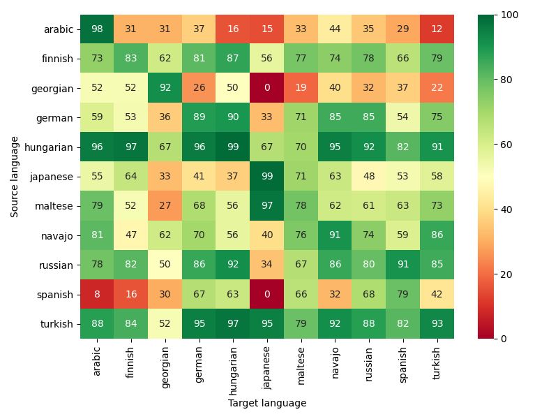
Contents

Acknowledgements                                                                                       1

Introduction                                                                                           2

1 Definition of the problem                                                                            4
  1.1   Tasks to address . . . . . . . . . . . . . . . . . . . . . . . . . . . . . . . . . . . .       4
        1.1.1   Classification . . . . . . . . . . . . . . . . . . . . . . . . . . . . . . . . . .     5
        1.1.2   Solving analogies . . . . . . . . . . . . . . . . . . . . . . . . . . . . . . . .      5
  1.2   Properties of analogies for data augmentation . . . . . . . . . . . . . . . . . . . .          7
  1.3   Our dataset(s) . . . . . . . . . . . . . . . . . . . . . . . . . . . . . . . . . . . . .       8
        1.3.1   SIGMORPHON 2016 dataset . . . . . . . . . . . . . . . . . . . . . . . . .              8
        1.3.2   Japanese Bigger Analogy Test Set . . . . . . . . . . . . . . . . . . . . . .           8
        1.3.3   Loading and augmenting the data . . . . . . . . . . . . . . . . . . . . . .            9
        1.3.4   (Dis)similarities between languages . . . . . . . . . . . . . . . . . . . . . .       11

2 Solving analogy related tasks                                                                       14
  2.1   First attempt with pre-trained GloVe embeddings . . . . . . . . . . . . . . . . . .           14
  2.2   Custom embedding model . . . . . . . . . . . . . . . . . . . . . . . . . . . . . . .          16
        2.2.1   Structure of our character-level embedding model . . . . . . . . . . . . . .          16
        2.2.2   Training phase and classification results . . . . . . . . . . . . . . . . . . .       16
  2.3   Solving analogies . . . . . . . . . . . . . . . . . . . . . . . . . . . . . . . . . . . .     20
        2.3.1   Evaluation method . . . . . . . . . . . . . . . . . . . . . . . . . . . . . . .       20
        2.3.2   Results . . . . . . . . . . . . . . . . . . . . . . . . . . . . . . . . . . . . .     21

3 Transfer learning                                                                                   25
  3.1   Full transfer . . . . . . . . . . . . . . . . . . . . . . . . . . . . . . . . . . . . . . .   25
  3.2   Partial transfer . . . . . . . . . . . . . . . . . . . . . . . . . . . . . . . . . . . . .    26
  3.3   Discussion . . . . . . . . . . . . . . . . . . . . . . . . . . . . . . . . . . . . . . . .    26

4 Conclusion and perspectives                                                                         28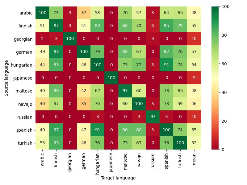
4.1   Improvement of the training settings . . . . . . . . . . . . . . . . . . . . . . . . .       28
  4.2   Towards a multilingual word embedding model? . . . . . . . . . . . . . . . . . . .           29
  4.3   Discussion about ideographic languages . . . . . . . . . . . . . . . . . . . . . . .         29
  4.4   Final remarks    . . . . . . . . . . . . . . . . . . . . . . . . . . . . . . . . . . . . .   29

Bibliography                                                                                         31

Appendix                                                                                             34

A Glossary                                                                                           34

B Statistics on the datasets                                                                         35

C Examples for the classification and analogy solving tasks                                          40
  C.1 Classification task . . . . . . . . . . . . . . . . . . . . . . . . . . . . . . . . . . .      41
  C.2 Solving analogies . . . . . . . . . . . . . . . . . . . . . . . . . . . . . . . . . . . .      43

D Analogy solving k-extended results                                                                 46
Acknowledgements

The achievement of this project could not have been possible without the contributions from
our respective people. We are highly thankful to our supervisors, Miguel Couceiro and Esteban
Marquer for their practical guidance, constructive advice and endless support throughout this
year. We would also like to thank Timothee Mickus for providing us with the Japanese Dataset,
which we used extensively in our empirical setting. Last but not least, we thank Pierre-Alexandre
Murena for his guidance, willigness to share his knowledge, and eagerness to help us. Lastly, we
are extremely grateful to all lecturers of IDMC for teaching us to gain a deeper understanding
on developing this project.
Introduction

Analogy consists of four objects or words A, B, C, and D and draws a parallel between the
relation between A and B and the one between C and D. Analogy can be used as a method of
reasoning and can be expressed by an analogical proportion, which is a statement such as “A is
to B as C is to D”. An analogical proportion becomes an equation if one of its four objects is
unknown (Miclet et al., 2008).
    Analogies have been extensively studied in Natural Language Processing, which resulted in
different formalizations with noteworthy applications in various domains such as derivational
morphology (Murena et al., 2020). Analogies on words can refer exclusively to their morphology
as in the following example:

                              R = {x | apple is to tree as apples is to x}.

Solving this form of equations can be done by calculating the set R of solutions x which satisfy
the analogy (Miclet et al., 2008). In this case, the observed solution is based on morphological
variations of two words: “apple” and “tree”. The question of the correctness of an analogy
A : B :: C : D is a difficult task; however, it has been tackled both formally and empirically
(Murena et al., 2020; Lim et al., 2019; Lepage, 2003). Recent empirical works propose a data-
oriented strategies to learn the correctness of analogies from past observations. These strategies
are based on machine learning approaches.
    In this project we focused on analogies, with a particular emphasis on morphological word
variations and how they determine the relation between different words. Our project was inspired
by the paper of Lim et al. (2019), which proposes a deep learning approach to train models of
semantic analogies on word embeddings 1 by using pre-trained GloVe 2 (Pennington et al., 2014)
embeddings. The results of this approach were competitive for analogy classification and solving.
This led us to adapting the neural framework presented in Lim et al. (2019) to morphological
analogies. The major difference is that our morphological approach relies on customized model
embeddings, which were fully designed and trained during this project.
    We used the Sigmorphon 2016 dataset (Cotterell et al., 2016) as well as the Japanese
Bigger Analogy Test Set dataset released by Karpinska et al. (2018) to analyze how deep
learning could help us classify and solve morphological analogies. These datasets covered 11
languages in total, 10 of which are from the Sigmorphon 2016 dataset (Cotterell et al., 2016),
while another one is from Japanese Bigger Analogy Test Set (Karpinska et al., 2018).
We used a character-level embedding to encode the morphemes of the words. To emphasize, we
focus on the structure of the words more than their meanings. Once the model is trained, it is
be able to embed any word, even those that did not appear during the training phase.
  1
     A word embedding is word representation that allows words with similar meaning to have a similar represen-
tation in vector space
   2
     GloVe is an open-source project at Stanford used for obtaining word embeddings

                                                      2
This report is organized as follows. We start by introducing analogical proportions, moti-
vation, objective, and related work. We also introduce the datasets we used and discuss their
properties in Chapter 1. Chapter 2 introduces the approaches that we used to classify and solve
morphological analogies. We also discus some results we obtained and some of the challenges
we encountered. Chapter 3 illustrates the adaptability of our framework by showing that mod-
els trained on a given language may be transferred to a different language. In fact, the latter
revealed noteworthy (dis)similarities between languages. In Chapter 4, we briefly discuss the
results that we have obtained and describe the current status of the project. Apart from that, we
also highlight some of the challenges encountered through the development process and present
some topics of future work, namely, potential improvements to the current project.
To realize this project, we used exclusively Python (version 3.9) (Van Rossum & Drake,
2009) and in particular the deep learning-oriented library PyTorch (Paszke et al., 2019). We
used various built-in Python libraries including Pandas, Matplotlib, Numpy and Scikit-learn
for minor uses like storing data and support functions. To train the deep leaning models,
we required substantial computational resources, so experiments presented in this paper were
carried out using the Grid’5000 (Balouek et al., 2013) testbed, supported by a scientific interest
group hosted by Inria and including CNRS, RENATER and several Universities as well as other
organizations (see https://www.grid5000.fr). All the codes we used during this project are
available on GitHub (see https://github.com/AmandineDecker/nn-morpho-analogy.git).
3Chapter 1
Definition of the problem
Analogical learning based on formal analogy can be applied to many problems in computational
linguistics. To quote Haspelmath (2002): “Morphology is the study of systematic co-variation
in the form and meaning of words.” When analyzing analogy in a morphological approach, we
are looking at the co-variation in the form of a single word. For example, “reader is to doer as
reading is to doing” is an analogy made of four tuples that present the different variations of the
lexicons “read” and “do” (Miclet & Delhay, 2003). Analyzing analogies based on morphology
allows the linguist to find how the word could vary based on gender, plurality, tense, mood,
etc. It also allows the linguist to predict how words change form based on these classified
patterns even if they are not familiar with certain words. When it comes to real life application,
morphological analogies are used as a method for acquiring new languages. It was one of the
evaluating methods used in assessment tests like SAT, TOEFL, and ACT, making around 20
percent of the questions posed (Turney, 2001; Betrand, 2016). These questions mainly focus on
inflectional affixes in morphology. Therefore, in this project we aimed to:
• build a model that automatically determines if four words form a valid analogy;
• build a model which can solve morphological analogical equations;
• determine whether different languages share morphological properties.
As mentioned, for this project we adapted a novel approach, particularly a deep learning
one, to deal with morphological analogies. Various models have been proposed to solve semantic
analogies including Textual Analogy Parsing approach (TAP), Dependency Relation approach
(DP), Vector Space Model (VSM), and Neural Network approach (NN) (Lamm et al., 2018; Chiu
et al., 2007; Turney, 2006; Lim et al., 2019). Out of these models, we were most interested in
VSM and NN approaches, and we finally decided to work with a NN and develop Lim’s approach
(Lim et al., 2019) due to the interesting results that they achieved. Though this approach is
more complex than VSM, it is in fact not that complex to implement to solving morphological
analogies. We adapted Lim et al.’s approach by customising morphological word embeddings as,
to our knowledge, there were no ready made ones for this task. Thus we trained and developed
an embedding model for this project.
1.1 Tasks to address
The two tasks tackled by (Lim et al., 2019) are identification of analogical proportions and
solving of analogical equations, which are both based on natural language. Words are encoded
4Figure 1.1: Structure of the CNN as a classifier. (Lim et al., 2019)
as numerical vectors with a word embedding process.
In terms of neural networks, identifying an analogical proportion consists in deciding whether
A : B :: C : D holds true or not: it is a binary classification task. Solving analogical propor-
tions can be seen as a regression task where we try to approximate the function f such that
f (A, B, C) = D if A : B :: C : D holds true.
Both tasks are further explained in the following subsections. In our project, we worked on
both of these tasks, where we train our custom embedding model on the classification task and
then use it to solve morphological analogies.
1.1.1 Classification
The classification task consists in determining if a quadruple (A, B, C, D) is a valid analogy or
not. The model is based on the structure provided in (Lim et al., 2019), the network can be
visualised on Figure 1.1.
As input of the model we have four vectors A, B, C, and D of size n. We stack them to get
a matrix of size n × 4. This matrix is the representation of the analogy A : B :: C : D, it means
that it should be analysed as a structure containing two pairs of vectors: (A, B) and (C, D).
The size h × w : 1 × 2 of the filters of the first CNN layer respects the boundaries between
the two pairs. This layer should analyse each pair and be able to notice the differences and
similarities between the elements of each pair.
The second CNN layer should compare the results of the analysis of both pairs: if A and B
are different in the same way as C and D then A : B :: C : D is a valid analogy.
Eventually all the results are flattened and used as input of a dense layer. We use a sigmoid
activation to get a result between 0 and 1 as we work with a binary classifier.
1.1.2 Solving analogies
Given the words A, B and C, solving analogical equations consists in producing the word D
such that A : B :: C : D holds true. From a machine learning perspective, a model which
can perform this task would take as input a triple (embed(A), embed(B), embed(C))1 and would
produce as an output a X, which ideally would correspond to the embedding of the word D
1
embed(X) refers to the embedding of the word X
5Figure 1.2: Structure of the neural network for analogy solving. (Lim et al., 2019)
such that A : B :: C : D holds true. The analogy solving task thus requires two models: one
producing a vector based on three others, like what we just described, and also an embedding
model which we discuss in Sections 2.1 and 2.2.
The model we used to produce D given (A, B, C) is taken from (Lim et al., 2019). The
assumption of the authors is that the X of the analogical equation A : B :: C : X can be found
thanks to a function f of A, B and C. This point of view redefines the analogy solving task. It
becomes a multi-variable regression problem based on the following dataset:
( )
A : B :: C : D belongs to the original
((embed(A), embed(B), embed(C)), embed(D))
set of valid analogies
The neural network they designed is described on Figure 1.2. The structure reflects the
relevance of the relations between the different words of the analogy. Indeed, for an analogy
A : B :: C : X, the link between A and B as well as the link between A and C is relevant to
determine X but also the relation between the pairs (A, B) and (A, C). This is the reason why
the function g(embed(A), embed(B), embed(C)), which determines X, is approximated by two
hidden functions f1 (embed(A), embed(B)) and f2 (embed(A), embed(C)). Overall, we have:
X = g(f1 (embed(A), embed(B)), f2 (embed(A), embed(C))).
In the neural network, f1 and f2 are approximated by two linear layers. The input is of size
2×n, where n is the embedding size, because the inputs are the concatenation of two embeddings
embed(A) and embed(B) or embed(A) and embed(C).
The output of each of these layers, of size 2 × n, are concatenated into a matrix of size 4 × n
and fed to a final linear layer which approximates g. The output is of size n which is the size of
an embedding so we can expect the model to produce a vector corresponding to the embedding
of X such that A : B :: C : X.
61.2 Properties of analogies for data augmentation
Deep learning approaches require a large amount of data. Therefore we took advantage of
some properties of analogies to produce more data based on our datasets, this process is called
data augmentation. Given one valid analogy, we can generate seven more valid analogies and
three invalid ones. Training our models on different equivalent forms of the same analogy helps
reducing overfitting. In this section, we describe the properties which enable us to augment our
datasets.
Analogies are classified and grouped based on the type of relation that exist between word
pairs. The first implementation of proportions was introduced by Ancient Greeks and was
used in the domain of numbers. Two examples worth mentioning are arithmetic proportion
and geometric proportion (Couceiro et al., 2017). These two examples illustrate the analogical
proportion statement of “A is to B as C is to D.”
• A, B, C, and D are proportional if A − B = C − D (arthimetic);
A C
• A, B, C, and D are proportional if B = D (geometric).
These quaternary relations obey the following axioms (Lepage, 2003):
(1) A : B :: A : B (reflexivity);
(2) A : B :: C : D → C : D :: A : B (symmetry);
(3) A : B :: C : D → A : C :: B : D (central permutation);
From these properties, we can infer the following 8 equivalent analogies to A : B :: C : D
(Cortes & Vapnik, 1995; Gladkova et al., 2016; Delhay & Miclet, 2004).
• A : B :: C : D (base form).
• C : D :: A : B (symmetry).
• A : C :: B : D (central permutation).
• B : A :: D : C.
(3) (2) (3)
Proof. A : B :: C : D ==⇒ A : C :: B : D ==⇒ B : D :: A : C ==⇒ B : A :: D : C;
• D : B :: C : A.
(3) (2)
Proof. C : D :: A : B ==⇒ C : A :: D : B ==⇒ D : B :: C : A.
• D : C :: B : A.
(2)
Proof. B : A :: D : C ==⇒ D : C :: B : A;
• C : A :: D : B.
(2)
Proof. D : B :: C : A ==⇒ C : A :: D : B;
• B : D :: A : C.
(2)
Proof. A : C :: B : D ==⇒ B : D :: A : C.
7Fremdsprache pos=N, c a s e=ACC, gen=FEM, num=PL Fremdsprachen
Figure 1.3: Example from the German training set for task 1.
In addition to these forms, we have 3 analogical forms which are considered invalid analogies
as they cannot be deduced from the base form A : B :: C : D and the axioms (1), (2), and (3)
and they contradict the intuition:
1. B : A :: C : D;
2. C : B :: A : D;
3. A : A :: C : D.
We used these properties to augment our datasets for the classification and solving tasks:
we produced eight valid analogies and three invalid ones given a valid A : B :: C : D for the
classification task and only the eight valid ones for solving analogies.
1.3 Our dataset(s)
For this project, we used the Sigmorphon 2016 dataset (Cotterell et al., 2016) and the
Japanese Bigger Analogy Test Set (Karpinska et al., 2018). As previously mentioned,
these datasets covered 11 languages in total, 10 of which are from the Sigmorphon 2016
dataset while the other one is from Japanese Bigger Analogy Test Set. In this chapter,
we introduce both of these datasets and explain some of the preprocessing conducted before the
realization part of the project.
1.3.1 SIGMORPHON 2016 dataset
One of the datasets we used was Sigmorphon 2016 (Cotterell et al., 2016), which contained
training, development and test data. Data is available for 10 languages: Spanish, German,
Finnish, Russian, Turkish, Georgian, Navajo, Arabic, Hungarian and Maltese. Most of them are
considered as languages with rich inflection (Cotterell et al., 2018). It is separated in 3 subtasks:
inflection, reinflection and unlabled reinflection. All the provided files are in UTF-8 encoded text
format. Each line of a file is an example for the task, the fields are separated by a tabulation.
In our experiments, we focused on the data from the inflection task, which is made up of triples
⟨A, F, B⟩ of a source lemma A (ex: “cat”), a set of features F (ex: pos=N,num=PL) and the
corresponding inflected form B (ex: “cats”). The forms and lemmas are encoded as simple
words while the tags are encoded as morphosyntactic descriptions (MSD), e.g., the grammatical
properties of the words such as their part of speech, case or number (among others).
A triple lemma, MSD, target form from the German training data is presented on
Figure 1.3
1.3.2 Japanese Bigger Analogy Test Set
The dataset we used for Japanese was generated from pairs of words of the dataset released by
Karpinska et al. (2018). This dataset contains several files, each of them containing pairs of
linguistically related words. The list of relations is described in Table 1.1.
8Relation Example Pairs
verb_dict - mizenkei01 会う → 会わ/あわ 50
Inflectional morphology
verb_dict - mizenkei02 出る → 出よ/でよ 51
verb_dict - kateikei 会う → 会え/あえ 57
verb_dict - teta 会う → 会っ/あっ 50
verb_mizenkei01 - mizenkei02 会わ → 会お/あお 50
verb_mizenkei02 - kateikei 会お → 会え/あえ 57
verb_kateikei - teta 会え → 会っ/あっ 50
adj_dict - renyokei 良い → 良く/よく 50
adj_dict - teta 良い → 良かっ/よかっ 50
adj_renyokei - teta 良く → 良かっ/よかっ 50
noun_na_adj + ka 強 → 強化/きょうか 50
Derivational morphology
adj + sa 良い → 良さ/よさ 50
noun + sha 筆 → 筆者/ひっしゃ 50
noun + kai 茶 → 茶会/ちゃかい 50
noun_na_adj + kan 同 → 同感/どうかん 50
noun_na_adj + sei 毒 → 毒性/どくせい 52
noun_na_adj + ryoku 馬 → 馬力/ばりき 50
fu + noun_reg 利 → 不利/ふり 50
dai + noun_na_adj 事 → 大事/だいじ 50
jidoshi - tadoshi 出る → 出す/だす 50
Table 1.1: List of relations between the words of the Japanese dataset.
We were interested in inflectional and derivational morphology relations for which the dataset
contains respectively 515 and 502 pairs of words. For each two pairs with the same relation, we
produced an analogy, which gave us 26410 analogies in the end. This set is smaller than the
Sigmorphon 2016 one, but this was not an issue when training the classification and embedding
model because we could produce 8 valid and 3 invalid analogies in total with a given valid one.
However, Japanese produced poor results when solving analogies which may be related to the
size of the dataset.
1.3.3 Loading and augmenting the data
To obtain morphological analogies from the Sigmorphon 2016, we defined our analogical pro-
portions as follows: for any two triples of the form:
⟨A, F, B⟩, ⟨A′ , F ′ , B ′ ⟩
which share the same morphological features (F = F ′ ), we considered A : B :: A′ : B ′ an
analogical proportion. Figure 1.4 presents two examples from the German training set for
building analogies.
Notice that only one analogy is generated for each pair of triples. For example, if we generate
A : B :: A′ : B ′ , we do not generate A′ : B ′ :: A : B as it is generated by the process introduced
in Section 1.2. During training and evaluation, for each sample of the dataset we generated
8 positive and 3 negative examples following the properties mentioned in Section 1.2. This
approach does not match the one of Lim et al., as they additionally generated the 8 equivalent
forms for each negative example.
The Sigmorphon 2016 dataset contains training and testing files for all of the languages.
9Fremdsprache pos=N, c a s e=ACC, gen=FEM, num=PL Fremdsprachen
Absorption pos=N, c a s e=ACC, gen=FEM, num=PL Absorptionen
absurd pos=ADJ, c a s e=DAT, gen=FEM, num=SG absurder
“Fremdsprache”:“Fremdsprachen”::“Absorption”:“Absorptionen” is a valid analogy.
“Fremdsprache”:“Fremdsprachen”::“absurd”:“absurder” is not because (“Fremdsprache”,
“Fremdsprachen”) and (“absurd”, “absurder”) do not share the same MSD.
Figure 1.4: Examples from the German training set for building analogies.
Language Train Dev Test
Arabic 373,240 7,671 555,312
Finnish 1,342,639 22,837 4,691,453
Georgian 3,553,763 67,457 8,368,323
German 994,740 17,222 1,480,256
Hungarian 3,280,891 70,565 66,195
Maltese 104,883 3,775 3,707
Navajo 502,637 33,976 4,843
Russian 1,965,533 32,214 6,421,514
Spanish 1,425,838 25,590 4,794,504
Turkish 606,873 11,518 11,360
Table 1.2: Number of analogies for each language before data augmentation.
For our project, we generated analogies by using these files. The number of analogies for each
language is presented in Table 1.2. For both the training and evaluation, we decided to work with
50,000 analogies to keep the training time reasonable (around 6 hours on Grid’5000). Maltese,
Navajo and Turkish were evaluated on less than 50,000 analogies because the related datasets
were too small as we can see in Table 1.2.
The Japanese dataset contains one file per transformation (listed in Table 1.1). We grouped
all these files together in one file following the same format of the Sigmorphon 2016 files:
lemma, transformation, target form. When we load the data, analogies are loaded based
on word pairs with the same relation, which yields 26410 analogies. We split the dataset to get
70 percent for training and 30 percent for testing. For reproducibility, the list of analogies for
training and testing were stored in separate files to ensure that the same sets were used every
time we evaluated.
To load the data and build the mentioned analogies, we used the “data.py” code provided
by Esteban Marquer. The “data.py” file contains the classes we use to import the data and
transform the words into vectors. The code can be manipulated using different modes (“train”,
“dev”, “test”, “test-covered”) and different languages (“Arabic”, “Finnish”, “Georgian”, “Ger-
man”, “Hungarian”, “Japanese”, “Maltese”, “Navajo”, “Russian”, “Spanish”, “Turkish”). An
augmentation function is introduced which, given an analogy, yields all the equivalent forms
based on the properties described in Section 1.2. Another function generated the invalid forms
described in Section 1.2. When we instantiate “Task1Dataset” class from the “data.py” file, it
generates a list of quadruples where each quadruple represents an analogy. The quadruples can
be in either plain words or lists of integers. We used plain words with the GloVe pre-trained
embeddings, e.g., for German only (Section 2.1). The lists of integers were used with our custom
embedding model. These lists are built with a dictionary mapping characters to integers: we
10first build the list of all the characters contained in the file and assign for each of them an integer
(e.g., an ID), then the encoding of a word is the list of IDs corresponding to the characters of
the word. For instance the German word “abfällig” is encoded as “[21, 22, 26, 50, 32, 32, 29,
27]”.
The dictionary thus depends on the input file. Note that the size and the content of the
embedding layer of our model depends on the size and the content of the dictionary, i.e., we
cannot use a file with a dictionary of size m with an embedding model of size n if n ̸= m.
Moreover, if the dictionary has the right size but the IDs are not matched with the same letters
as in the dictionary used during training, the results can be unexpected. This topic is discussed
later in Section 2.2.
1.3.4 (Dis)similarities between languages
In order to compare the different languages, and have more material to explain our results later,
we computed some statistics on the datasets.
1.3.4.1 Statistics about the words of the languages
Words length For all the languages except Japanese, the mean of the words (Appendix B
and Table B.1) length lies between 7.6 and 11. For Japanese, the words mean length is of
5 ± 3 (mean length ± standard deviation), this dataset contains very short words (one or two
characters) as well as longer ones (up to eighteen characters).
Differences between training and testing set For all the languages except Japanese,
between 58% and 87% of the words of the test set are new compared to the words of the
training set (Table B.2). It means that the models were evaluated on new analogies but also
partially on analogies based on words never encountered. It was not the case for Japanese
because of the way we built the dataset. Indeed, we first generated all the possible analogies
based on the pairs of words we had and then split them between a training and a test set. If
we had split the pairs of words instead, we would have had new words in the test set but the
training and test sets would have been smaller than they currently are. As a comparison, the
datasets from Sigmorphon 2016 contain at least 104,883 analogies for training against 18,487
for the Japanese Bigger Analogy Test Set.
Number of transformations We call a transformation the process used to go from the first
word to the second in a word pair. For languages of Sigmorphon 2016 they are described by
an MSD and for Japanese they are the relations described in Table 1.1. Most languages have less
than 100 different transformations in the training set (Table B.1) and between 100 and 200 word
pairs per transformation in average (Figure B.2). Arabic and Turkish have more transformations
(187 and 223) and fewer pairs per transformation (54 and 65 in average) but since there are
n(n+1)
2 analogies generated for n word pairs with a given transformation, it should not impact the
learning process. For Maltese however, there are more than 3,000 different transformations for an
average of 5 word pairs per transformation. If the morphemes implied in these transformations
are very different for each other it could be a problem for the model as there is very few data for
each transformation but a lot of different patterns to learn. Moreover, the test set of Maltese
contains 105 new transformations compared to the test set which could be a problem if these
transformations imply different modifications from the ones involved in the transformations of
11the training set as the model would never have encountered them. Arabic, German and Russian
test set also contain new transformations compared to their respective testing sets but to a lesser
extent (6 for Arabic, 2 for German and Russian).
Levenshtein distance The Levenshtein distance (Levenshtein, 1965) between two strings is
the minimal number of characters to edit (add, delete or modify) to change one string into the
other. We computed this distance on each pair of words of the datasets (Figure B.3) in order
to evaluate the amount of differences between the first and second word. Our assumption was
that a larger distance can imply more complex transformations and thus require a more complex
model. The average distance goes from 1.7 to 7.0. The languages with the smallest distance are
Georgian, German, Russian and Spanish and the ones with the biggest distance are Japanese
and Maltese. The range of Japanese words length is rather wide which could explain a high
Levenshtein distance if one word of the pair is short and the other long.
1.3.4.2 The sets of character dictionaries
The first step when we embed a word with our model consists in encoding this word with a list
of IDs. Each ID corresponds to a character present in the dataset, the German word “abfällig”
is encoded as “[21, 22, 26, 50, 32, 32, 29, 27]. We call character dictionary the mapping from
the characters to the IDs for one dataset. The character dictionaries vary from one dataset to
another as they contain only the characters used in the dataset.
Character dictionary lengths If we exclude Japanese which uses 632 characters, the lengths
of the set of characters in each dataset vary from 30 to 58 (Table B.2). In German, nouns start
with a capital letter. German thus uses the biggest character dictionary as it is the only one
containing capital letters. The Arabic is also longer than most because of the accented characters.
Comparisons between the character dictionaries of the languages For Finnish, Mal-
tese and Russian, the test set contains one character absent from the training set. To get the
full view of the differences in dictionaries between the languages, we computed the coverage of
the test dictionaries by the training dictionaries (Figure B.4). We computed it this way because
the models are trained on the training sets (and thus learn the related characters) and then
evaluated on the test sets (and thus need to deal with the characters of the test set). For a given
language, training to test coverage is 100% except for Finnish, Maltese and Russian for which
it is 97%. In average, all the languages except Georgian, Japanese and Russian have a coverage
of more than 45% (if we do not take Georgian, Japanese and Russian into consideration it rises
up to 60%) on other languages. Georgian, Japanese and Russian use a different alphabet than
the other languages which explains their poor coverage of and by other languages.
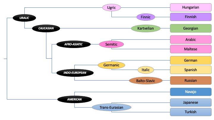
1.3.4.3 Language families
We investigated the proximity of the languages we work with thanks to their families. (Cole &
Siebert-Cole, 2020) provides the family tree of 10 out of 11 languages. Maltese is not represented
but based on (Harwood, 2021) we chose to represent it next to Arabic in the Afro-Asiatic family
as a Semitic language. In Figure 1.5, the languages are linked to their group or family which
are also linked together. Languages closer together belong to the same family as for Spanish
and German. Groups and families are also linked to one another depending on their history.
12Figure 1.5: Language tree of the 11 languages in the datasets.
For example, Georgian belongs to the Caucasian family, which descends from the Uralic family
that includes Hungarian and Finnish. Languages from the Afro-Asiatic family are closer to the
languages of the Uralic family than those of the American family.
13Chapter 2
Solving analogy related tasks
Before introducing this chapter, we are proud to say that most of the results discussed in Sec-
tions 2.2 and 2.2.2 led to the writing of a paper which was submitted to the IEEE International
Conference on Data Science and Advanced Analytics 2021.
For our project, we based our experiments on the two tasks described in Lim et al. (2019), i.e.,
analogy classification and solving of analogical equations, which requires a way to represent words
numerically. They worked with the pre-trained word embeddings for English provided by GloVe
Pennington et al. (2014). However, we worked with 11 languages (10 from Sigmorphon 2016 as
well as Japanese (Karpinska et al., 2018)) for which GloVe embeddings are not necessarily avail-
able. We could have used similar tools which cover more languages such as Grave et al. (2018)
which covers 157 languages. However, our experiments with GloVe (Section 2.1) showed us that
pre-trained word embeddings model tend not to cover the entirety of our dataset. Moreover,
these classical word embeddings are trained on word co-occurrence among the training texts,
they are thus usually able to solve semantic analogies such as “man′′ : “woman′′ :: “king ′′ : X
through co-occurrence similarities. But we dealt with morphological analogies and, for most
languages, morphology is not sufficiently linked to semantics for these models to perform as
good as we would like.
For all these reasons we developed a custom word embedding model focused on morphology.
Our model was trained along the classifier for a given language. The idea was to learn sub-words
and morphemes from single words (as opposed to texts for classical word embedding models).
This difference enabled us to embed any word even if it was not encountered during the training
phase, and to model morphology through the sub-words and morphemes.
2.1 First attempt with pre-trained GloVe embeddings
Our first experiment consisted in using GloVe embeddings with the regression model for which
Esteban Marquer wrote the code following the structure of Lim et al. (2019). We used the
German data of the first task of Sigmorphon 2016 to build a set of valid analogies with
the method described in Section 1.3.3. We obtained a set of 994, 740 quadruples of the form
⟨“abchasisch”, “abchasischerem”, “abchasisch”, “abchasischerem”⟩ which correspond to valid
analogies: a quadruple ⟨A, B, C, D⟩ corresponds to the valid analogy A : B :: C : D.
When the data is loaded, each word of the quadruple is embedded with GloVe into vectors
of size n = 300. We chose n = 300 as it is the biggest embedding size used by Lim et al. (2019)
and a bigger size most likely provides better results.
14As explained in Section 1.2, given one valid analogy, we are able to generate 7 more with
permutations. Our dataset thus contains 8 × 99, 4740 = 7, 957, 920 quadruples representing valid
analogies. We trained our model on this augmented dataset.
Our first experiments enabled us to determine that one epoch took around 3 hours to run.
We decided to train our model for 50 epochs, but we realised that the loss didn’t decrease at
the end of the training (it oscillated), which indicates that the model did not learn.
It could partly be explained by the fact that GloVe embeddings do not take morphology
into account, but this explanation alone was not satisfactory. We thus decided to find a way to
decrease the running time so that we could investigate the issues. We tried to use bigger data
batches and to store the embedded quadruples in a file we would load instead of embedding each
word during the training phase. However, none of these ideas significantly reduced the running
time. We concluded that the size of the dataset was probably responsible for the time needed
and decided to train a new model on 50, 000 analogies only (before augmentation) for 20 epochs.
These training conditions are the same as for the embedding model described in Section 2.2.2,
which is the one we used for all our other experiments.
As expected based on the results on the full dataset, the loss did not decrease on the smaller
dataset. When we evaluated the model (see Section 2.3.1), the accuracy was of 100% which did
not match the results from the loss. For this reason, we investigated the embeddings and noticed
that many words were embedded with a vector full of zeros. After further analysis, we discovered
that 49% of the words in the training set and 51% of the words in the test set were not present in
the GloVe file we used to embed our words and were thus embedded by the default zero vector.
Since an analogy is based on 4 words, it means that more than half of the analogies used for
training contained at least one word embedded with a zero vector. This could explain why the
model does not learn. Indeed, the model was trained on tuples (embed(A), embed(B), embed(C))
and was expected to produce embed(D), where A : B :: C : D holds true. But if one of the word
was embedded with a zero vector, the analogy did not hold anymore, so the data we used for
training the model contained invalid analogies that were (wrongfully) considered valid.
Moreover, if A, B, C and D are embedded as zero vectors, the model is taught that producing
a zero vector is the right thing to do. Therefore, since this kind of data was probably fed many
times to the model, it probably produced a zero vector all the time. As for the accuracy of
100%, we confirmed that all the expected and produced vectors were full of zeros.
After such results, we decided to abandon GloVe embeddings and started working on a
character embedding model which is more relevant for a morphology task. At this stage, we had
several options.
The first one consisted in training a character-level encoder trained with the regression model
(Figure 1.2). The encoder would have embedded A, B, C and D separately and then the model
would have run on these embeddings instead of the GloVe ones. However, this option has a
major issue. The solution of the analogical equation A : A :: A : X is always A, thus the
model would always be correct if it learned a dummy embedding (the same embedding for all
the possible inputs) and produced the same dummy embedding as a result.
The second option was also to create a character-level encoder, but trained on the classifica-
tion task (Figure 1.1). Contrary to the regression task, negative examples are directly available
for the classification task thanks to the permutation properties of analogies. These negative
examples would force the model to learn real embeddings.
Eventually the last option was to create an auto-encoder trained separately. This model
could work directly on the analogy solving task and would enable us to produce an actual word
15(and not an embedding) as output of the regression model. However, the literature does not
seem very developed for character level auto-encoders while we had some leads for an encoder.
Hence, this task seemed too complicated for us. It still remains an interesting lead for future
work.
2.2 Custom embedding model
Our aim was to solve morphological analogies. Our assumption was that we needed to investigate
the structure of the words more than their meanings. For this reason, a character embedding
model was more relevant than GloVe embeddings. Moreover, a character-level embedding model,
once trained, is able to embed any word even those not encountered during the training phase,
which solves the issue of the zero vector for unknown words (Vania, 2020).
2.2.1 Structure of our character-level embedding model
The structure described in Kim et al. (2016) is a CNN-LSTM language model where the CNN
part embeds the words while the LSTM part investigates the relation between the words, i.e.,
the context. As our aim was to embed words based on their morphological properties, the
context was meaningless for our task. Our embedding model was thus inspired from the CNN
part only.
Figure 2.1 describes the structure of our model. We first use a character embedding layer to
encode each character of the word with a vector of size m. Characters never encountered during
the training phase are embedded with vectors full of 0. At the beginning and at the end of the
word, we add special vectors to signify the boundaries of the word. For a word of |w| characters,
we obtain a (|w| + 2) × m vector. We chose m = 512 for Japanese and m = 64 for the other
languages. If we put Japanese aside, the biggest character dictionary contains 58 characters so
we chose m = 64 because it is the closest power of 2 to 58 + 2. Japanese’s dictionary contains
632 characters so we chose m = 512.
Then the idea is to apply filters of different sizes on the embedding, each filter should
recognize a pattern in the word: a filter of size 2 could recognize affixes such as “ab-”, “be-”,
“in-” or “-en” in German for instance. We did not find literature on the maximal length of
morphemes for our languages but we looked at an affix dictionary for German (IDS, 2018) in
order to have an idea about it. Most of the affixes were of length 2 to 4 so we decided to use
filters of size 2 to 6 to cover as many patterns as possible. We did not investigate the other
languages but we could improve our model in the future with more information about the size
of the morphemes. For each size we arbitrarily chose to use 16 filters. Further experiments are
needed to determine the most efficient number of filters and the different sizes to use.
After the CNN layers, a max pooling layer is applied: we keep only the greatest number
produced by each of the 80 filters (16 filters of 5 widths) so that only the most important patterns
appear in the final embedding. We finally concatenate the results to produce an embedding of
size 80.
2.2.2 Training phase and classification results
We decided to train this encoder with our classification model. Since we had both positive and
negative data thanks to the properties of analogies (see Section 1.2), the encoder did not learn
161.20 -0.71 0.28 0.27 0.66 -0.29 -0.29 -0.01 0.04 0.05
1.51 -0.60 -0.56 1.1 -0.28 0.29 0.29 -1.56 1.66 -2.30
0.85
1.10
0.69
0.75
1.22
0.85
max
0.47 -0.14
-0.03 0.59
-0.86 0.68
-0.12 0.18
-0.41 0.11
0.11 0.25
0.56 -0.40
-1.19 0.81 0.85 2.19
-0.76 0.41 0.15 -0.55 -0.02 0.21 1.10
-0.05 0.69 -0.69 1.10
0.69 0.28
0.92
0.36
BEG 59 1.20 1.51 0.78
1.12
a 21 -0.71 -0.60 1.20 -0.71 0.28 0.27 0.66 -0.29 -0.29 -0.01 0.04 0.05
0.33
1.51 -0.60 -0.56 1.1 -0.28 0.29 0.29 -1.56 1.66 -2.30
1.57
b 22 0.28 -0.56
0.58
f 26 0.27 1.1 0.53
ä 50 0.66 -0.28
-0.33
max 0.21
word: -0.56 -0.48
-0.42 -0.42 -0.52
0.66 -0.10 -0.39
-0.03 -0.25
0.01 -0.45 -0.22
-0.17 0.07 -0.46
-0.14 -0.77 0.06
-0.160.40
0.60 -0.09
0.06
0.4 0.06
0.66
abfällig l 32 -0.29 0.29 0.40
0.66
l 32 -0.29 0.29
0.81
…
i 29 -0.01 -1.56
g 27 0.04 1.66
0 0 0 1.20 -0.7 0.28 0.27 0.66 -0.2 -0.2 -0.0 0.04 0.05 0 0 0
END 60 0.05 -2.30 1 -0.5 1.1 -0.2 0.29
0 0 0 1.51 -0.6 9 0.29
9 -1.5
1 1.66 -2.3 0 0 0
0 6 8 6 0 0.79
1.12
0.56
0.48
max
0.16 -0.86
-0.26 -0.61
-0.35 -0.12
0.18 -0.15
-0.06 0.04
-0.37 -0.43
0.21 -0.32
-0.65 0.83
0.05 -0.54
-0.27 0.28
-1.06 0.83
0.21
0.06 -0.24 0.59 -0.08 -0.25 -0.38 0.27 -0.30 0.64 -0.06 0.52 0.64
Pre-embedding Embedding layer Convolution layer with multiple filters of different widths Concatenation
Max-pooling layer
with a char:int
16 filters of width n for n ∈ [2,6] 16x5 elements result of size 80
dictionary
Figure 2.1: Structure of the CNN as a character level embedding model.
17dummy embeddings as it could have done without negative data. Indeed with only positive
data, learning the same embedding for all the words would make all the analogies look like
A : A :: A : A, which is valid and the model would always be right. But if the model is trained
on both positive and negative data, the previous dummy embeddings would lead it to classify
invalid analogies as valid as the four elements would be equal. Using both positive and negative
data forced it to learn meaningful embeddings.
We used the Sigmorphon 2016 dataset for the training which enabled us to train 10 models
(one for each language). Since the training and testing sets are distinct in this dataset, it
is possible that the training file contains characters the testing file does not contain or the
opposite (Table B.2). In the first case, it implies that many characters of the character to
integer dictionary can have a different IDs during the training and the test part, so it yields
poor results. We fixed this issue by using the dictionary produced for training as the dictionary
for the test. However, this technique does not work in the opposite case, when the test file
contains characters the training file does not contain.
A solution to both these issues would be using the UTF-8 codes as IDs, but the vocabulary
would become very large as well as the embedding model since both are related. Another solution
would be using an ID for the unknown characters, the same way context based word embeddings
model use a vector for unknown words. Nevertheless, this solution would require that we retrain
all of our models with one more character. To avoid this problem, we decided to use embeddings
full of 0 for the unknown characters.
Most of the Sigmorphon 2016 files yield several hundreds of thousands analogies and each
analogy was used 11 times by the model (8 valid forms, 3 invalid). Using the entire datasets for
the training would have taken a very long time, as it did with GloVe, so we decided to use only
subsets of 50, 000 analogies and train for 20 epochs (which takes around 6 hours).
We also tried our model on Japanese, an ideographic language, to see if the results were
similar. The classification task produced very good results (they are among the best ones) but
the test set was small and even if the analogies of the test set were not used for training, they
were based on the same words, while the test sets of other languages contain new words. For
these reasons, Japanese could be less complex to deal with for the model.
The results of the classification task are described in Table 2.1. Most of the time, the
classification of invalid analogies is less accurate than valid analogies. We thought about two
major reasons for this. The first one is the presence of exceptions in the datasets (irregular verbs
for instance). Such transformations are less likely to be shared by many words and are thus not
recognised by our model. The second reason is the training setting. Since the model is trained
on 3 invalid analogies and 8 valid analogies, in practice 150, 000 invalid analogies and 400, 000
valid ones in total, it is possible that the model needs to be trained on more invalid data to
reach similar results as with valid data. We could apply the permutations properties on the 3
invalid analogies so that we would have 3 × 8 invalid analogies for 8 valid ones. However this
could lead the model to focus more on invalid analogies and thus induce a drop in the accuracy
for valid analogies. Moreover, we use valid and invalid data to make sure the embedding model
does not learn dummy embeddings and an imbalance between the number of positive examples
and the number of negative example could produce this result.
Examples for classification task on Arabic and German are shown in Table 2.2. Examples
for all the languages are available in appendices (Tables C.1 and C.2).
18Language Valid analogies Invalid analogies
Arabic 99.89 97.52
Finnish 99.44 82.62
Georgian 99.83 91.71
German 99.48 89.01
Hungarian 99.99 98.81
Japanese 99.99 98.65
Maltese 99.96 77.83
Navajo 99.53 90.82
Russian 97.95 79.85
Spanish 99.94 78.33
Turkish 99.48 92.63
Table 2.1: Accuracy results (in %) for the classification task. The Japanese model was trained
on 18, 487 analogies and tested on 7, 923 of the same dataset (the two subsets were distinct). All
the other models were trained on 50, 000 analogies and tested on 50, 000 of different sets except
for Maltese, Navajo and Turkish which were tested on 3, 707, 4, 843 and 11, 360 analogies due
to the size of the dataset.
No. Lang. Expected Result Analogy Form
1 ARA valid valid naffaqa:naffaqnā::dammama:dammamnā A:B::C:D
2 ARA valid invalid bayyāʿūna:al-bayyāʿu::nawarun:an-nawariyyu B:A::D:C
3 ARA invalid invalid dammama:naffaqnā::naffaqa:dammamnā C:B::A:D
4 ARA invalid valid al-ʾamtiʿatu:al-matāʿu::al-qīmatu:al-qiyamu B:A::C:D
5 GE valid valid extrovertiert:extrovertiertere::angelsächsisch:angelsächsischere A:B::C:D
6 GE valid invalid entgehen:entgingen::schwächen:schwächten A:B::C:D
7 GE invalid invalid extrovertiertere:extrovertiert::angelsächsisch:angelsächsischere B:A::C:D
8 GE invalid valid unkommunikative:unkommunikativ::abgestrahlt:abgestrahlte B:A::C:D
Table 2.2: Classification examples of Arabic (ARA) and German (GE). We call the words A,
B, C, and D depending on the order they appear in the dataset. A always forms a pair with B
and C always forms a pair with D.
For Arabic, in example (2), the reason the model fails might be due to the presence of a dicrtic
character in B that the model interprets as an affix. The model, therefore, reads the transfor-
mation between B and D as not corresponding to one another. For example (4), the analogy is
invalid because of its form but the model fails to notice it, which may be related to the smaller
amount of negative data during the training compared to positive data.
For German, example (6) uses an irregular verb, which probably explains why the model fails.
As for example (8), the analogy is invalid because of its form, like example (4), which the model
also fails to notice.
192.3 Solving analogies
The classification task enabled us to train embedding models which hopefully represent accu-
rately the morphology of the words. This leads us to the analogy solving task. Indeed, for an
analogical equation A : B :: C : X, the embeddings must encode the morphological features of
A, B and C so that the relation between A and B is also to be found between embed(A) and
embed(B). As explained in Section 1.1.2, we use the neural network proposed by Lim et al.
(2019) to solve this task.
The main issue with our approach is that we use a CNN encoder and not an auto-encoder.
It means that when the neural network for regression produces a vector, we have no tool to
transform this vector into a word. In order to match the produced vectors with actual words,
we considered all the embeddings of the words in the dataset for a given language and assumed
the closest vector to the produced one would be chosen as output. This method raises several
questions especially regarding the metrics we use and the way to deal with words equally close
to each others.
Our aim was to compare our results to those of Murena et al. (2020) who proposed an
empirical approach to solve morphological analogies which produced competitive results.
2.3.1 Evaluation method
Before training our models, we had to decide on an evaluation method. As mentioned before,
we worked with a word encoder and thus obtained vectors we cannot decode as output from the
regression neural network. These vectors were not equal to the expected ones so comparing the
expected vectors to the produced ones gave an accuracy of 0%. However, if we choose a method
to match a produced vector with one corresponding to the embedding of a word of the dataset
and this vector corresponds to the expected ones, we can consider the produced vector as right.
Given a produced vector, the idea was to find the closest one in a set of known embeddings.
To do this, we first stored the embeddings of all the words in the dataset of a given language,
e.g. the words of the testing set as well as those of the training set. As we evaluated our model
on the testing set, we did not need the embeddings of the words of the training set. However,
if we search among a bigger set, the accuracy we compute is more meaningful as it reduces the
possibility to get the right vector out of luck.
Then we had to choose a (dis)similarity metrics. The Cosine similarity and the Euclidean
distance given by Equation (2.1) and Equation (2.2), respectively, are the most commonly used:
X ·Y
Cosine_similarity(X, Y ) = (2.1)
∥X∥∥Y ∥
v
u n
uX
Euclidean_distance(X, Y ) = t (xi − yi )2 (2.2)
i=1
where X = (x1 , . . . , xn ) and Y = (y1 , . . . , yn ). Hence we decided to use both and compare
the results. More precisely, given a produced vector X, we computed its Cosine similarity
(resp. Euclidean distance) with all the stored embeddings and retrieved the vector Y such that
maximizes Cosine_similarity(X, Y ) (resp. minimizes Euclidean_distance(X, Y )).
This method enabled us to match each produced vector with one belonging to the stored
embeddings. As the expected tensors are embeddings of words present in this set as well, if
the produced vector is the right one then the one closest to it should be exactly the expected
20one. However, the process we used to store and then load the embeddings slightly modified
the tensors values: from the fifth decimal, the values of the components of the produced tensors
differ from the values of the components of the stored tensors. To tackle this issue, we considered
that the expected vector and the closest one were the same if their components were equal two
by two up to the fourth decimal.
With this method, there was a possibility that several vectors were equally close to the
produced one. During our first evaluation, we decided to use the first found vector with the
biggest similarity (resp. smallest distance). Later, we decided to check if the expected vector
was slightly further and thus considered all the vectors in a given similarity (resp. distance)
range.
2.3.2 Results
We trained the models for each language separately. For all of them, the training set consisted
in 50,000 analogies. The four words were embedded thanks to the trained CNN neural network
corresponding to the language of the data. Then for each quadruple of vectors, we used the
eight valid permutations as input data: for a valid permutation of the form A : B :: C : D,
we applied the regression model on (embed(A), embed(B), embed(C)) and compared the result
to embed(D) with mean squared error before the back-propagation. In the end, the model was
trained on 400,000 analogies.
2.3.2.1 First evaluation
As explained before, the evaluation method was such that the produced vector could be matched
with several vectors of the set of stored embeddings. For our first evaluation, we compared the
expected vectors only with the first matching vector among the stored ones (e.g. the one with
the smallest identifier). The results are described in Table 2.3, the last column contains the
results of (Murena et al., 2020) for the same task.
Japanese produced the worst results which could be explained by the length of the dataset
as well as the distribution of the embeddings. Also, our results are not as good as those of
(Murena et al., 2020) on all the languages. However, the language on which it performed best
is Georgian with both approaches, and the two worst languages (apart from Japanese) are also
the same. This indicated that our approach was relevant.
2.3.2.2 Further evaluation
Our results for solving analogies were far from the ones of (Murena et al., 2020) for most
languages but they were encouraging. Thus we wanted to know if the right vector was far
from the predicted one when our model failed. If not, it would indicate our neural approach is
relevant and could achieve better results with more training and/or fine-tuning. To do this, we
implemented a new evaluation method.
1. Given A, B, and C our model produces Dpredicted ;
2. We then compute the Cosine similarity (resp. Euclidean distance) between Dpredicted and
all the stored embeddings;
3. We order the stored embeddings according to their Cosine similarity (resp. Euclidean
distance) with Dpredicted so that the vector of rank 1 is the closest to Dpredicted ;
21Language Cosine similarity Euclidean distance (Murena et al., 2020)
Arabic 51.41 51.53 87.18
Finnish 72.84 72.23 93.69
Georgian 93.37 93.44 99.35
German 87.55 87.78 98.84
Hungarian 68.31 68.13 95.71
Japanese 19.76 17.50 /
Maltese 75.68 76.94 96.38
Navajo 45.81 47.41 81.21
Russian 69.57 69.05 96.41
Spanish 87.86 87.53 96.73
Turkish 70.10 67.77 89.45
Table 2.3: Accuracy results (in %) for the analogy solving task. The Japanese model was trained
on 18, 487 analogies and tested on 7, 923 of the same dataset (the two subsets were distinct). All
the other models were trained on 50, 000 analogies and tested on 50, 000 of different sets except
for Maltese, Navajo and Turkish which were tested on 3, 707, 4, 843 and 11, 360 analogies due
to the size of the dataset.
4. We retrieve the rank 1 vector Dclosest ;
5. We retrieve the next vectors in the ordered list until the Cosine similarity (resp. Euclidean
distance) is too small (resp. too large) compared to the one of the vector of rank 1, we
use a parameter k to make the maximal difference vary;
6. If the expected vector is among the retrieved ones then we consider the model was right
and we retrieve the rank of the right vector for statistics;
7. If the expected vector is not among the retrieved ones then we consider our model failed
and add a 0 to the list of ranks.
In practice, if Cosine_similarity(Dpredicted , Dclosest ) = s0 , we retrieved all the vectors t such
that Cosine_similarity(Dpredicted , t) ≤ (1 − k) ∗ s0 for k ∈ {0, 0.01, 0.02, 0.05}. We used k = 0
to see if there were often several vectors which shared the same similarity (resp. distance) from
the predicted one, which is not the case (the length of the sets of retrieved vectors are available
in appendices: Table D.1). Table 2.4 provides a few examples of the words produced by the
model for k = 0.02. Examples for all the languages are available in appendices (see Tables C.3
to C.5).
Several factors influence why the Arabic model would fail. Even when the size is set, the
variety of affixes in Arabic could affect the validity of the analogy. Both pairs should follow the
same pattern (have the same format and use the same affix) for the model to be valid. Another
factor is the fact that the model might interpret that some words contain an affix, when, in fact,
they don’t (for instance the word “determine” seems to contain the affix “de-”). As for the third
Arabic example, we aren’t sure why the model failed. The same words were used in the previous
examples but presented in a different order (words belonging to the same pair are placed next
to one another) and the model was able to find the expected result. Therefore, we aren’t able
to provide an explanation as to why the model failed to find the expected result for the third
example.
22You can also read