Forecasting the Evolution of North Atlantic Hurricanes: A Deep Learning Approach - NIST Technical Note 2167

Page created by Bill Johnson
 
CONTINUE READING
Forecasting the Evolution of North Atlantic Hurricanes: A Deep Learning Approach - NIST Technical Note 2167
NIST Technical Note 2167

    Forecasting the Evolution of North
Atlantic Hurricanes: A Deep Learning
                            Approach

                                                 Rikhi Bose
                                              Adam L. Pintar
                                                 Emil Simiu

                This publication is available free of charge from:
                          https://doi.org/10.6028/NIST.TN.2167
NIST Technical Note 2167

        Forecasting the Evolution of North
    Atlantic Hurricanes: A Deep Learning
                                Approach
                                                                                     Rikhi Bose
                                                       Materials and Structural Systems Division
                                                                        Engineering Laboratory

                                                                                    Adam L. Pintar
                                                                   Statistical Engineering Division
                                                                            Engineering Laboratory

                                                                                     Emil Simiu
                                                       Materials and Structural Systems Division
                                                                        Engineering Laboratory

                                               This publication is available free of charge from:
                                                         https://doi.org/10.6028/NIST.TN.2167

                                                                                             June 2021

                                                                          U.S. Department of Commerce
                                                                           Gina M. Raimondo, Secretary

                                                           National Institute of Standards and Technology
James K. Olthoff, Performing the Non-Exclusive Functions and Duties of the Under Secretary of Commerce
                  for Standards and Technology & Director, National Institute of Standards and Technology
Certain commercial entities, equipment, or materials may be identified in this document in order to describe
             an experimental procedure or concept adequately. Such identification is not intended to imply
recommendation or endorsement by the National Institute of Standards and Technology, nor is it intended to
           imply that the entities, materials, or equipment are necessarily the best available for the purpose.

                      National Institute of Standards and Technology Technical Note 2167
                        Natl. Inst. Stand. Technol. Tech. Note 2167, 36 pages (June 2021)
                                                                      CODEN: NTNOEF

                                               This publication is available free of charge from:
                                                          https://doi.org/10.6028/NIST.TN.2167
______________________________________________________________________________________________________

                                                                                                           Abstract

                                                                                                           Accurate prediction of storm evolution from genesis onwards may be of great importance
                                                                                                           considering that billions of dollars worth of property damage and numerous casualties are
                                                                                                           inflicted each year all over the globe. In the present work, two classes of Recurrent Neural
                 This publication is available free of charge from: https://doi.org/10.6028/NIST.TN.2167

                                                                                                           Network (RNN) models for predicting storm-eye trajectory have been developed. These
                                                                                                           models are trained on input features available in or derived from the North Atlantic hurri-
                                                                                                           cane database maintained by the National Hurricane Center (NHC). The models utilize his-
                                                                                                           torical data to estimate probabilities of storms passing through any location. Furthermore,
                                                                                                           inputs to the models are such so that the model development methodology is applicable to
                                                                                                           any oceanic basin in any part of the globe. Model forecasting errors have been analyzed in
                                                                                                           detail. The error analysis shows that the Many-To-Many class of models are appropriate for
                                                                                                           long-term forecasting while Many-To-One prediction models perform comparably well for
                                                                                                           6 − hr predictions. Application of these models to predicting more than 40 test storms in
                                                                                                           the North Atlantic basin shows that, at least for forecasts of up to 12 hours, they outperform
                                                                                                           all data-based storm trajectory prediction models cited in the paper. Apart from providing
                                                                                                           very fast predictions, the RNN models require less information than models used in current
                                                                                                           practice. Because the models presented herein emulate the trajectory trends of historical
                                                                                                           storms, they are currently being used for the simulation of synthetic storm tracks and fea-
                                                                                                           tures and the subsequent estimation of extreme wind speeds with various mean recurrence
                                                                                                           intervals.

                                                                                                           Key words

                                                                                                           Hurricane forecasting; HURDAT2; Long Short-Term Memory (LSTM); North Atlantic
                                                                                                           hurricanes; Recurrent Neural Networks (RNN); Time series forecasting.

                                                                                                                                                         i
______________________________________________________________________________________________________

                                                                                                                                          Table of Contents
                                                                                                           1 Introduction                                                                          1
                                                                                                           2 Database: HURDAT2                                                                    4
                                                                                                             2.1 Feature space                                                                    4
                 This publication is available free of charge from: https://doi.org/10.6028/NIST.TN.2167

                                                                                                             2.2 Statistics                                                                       6
                                                                                                             2.3 Zonal data                                                                       7
                                                                                                           3 Model development                                                                    11
                                                                                                             3.1 Classification                                                                   11
                                                                                                             3.2 Regression                                                                       12
                                                                                                             3.3 Model: LSTM RNN                                                                  13
                                                                                                             3.4 Model: Architecture & Implementation                                             15
                                                                                                             3.5 Model: Training strategies                                                       17
                                                                                                             3.6 Hyperparameter tuning                                                            18
                                                                                                           4 Results                                                                              20
                                                                                                             4.1 Mean forecast error                                                              20
                                                                                                             4.2 Storm trajectory prediction                                                      22
                                                                                                             4.3 Limitations                                                                      24
                                                                                                           5 Conclusions                                                                          27
                                                                                                           References                                                                             29

                                                                                                                                             List of Figures
                                                                                                           Fig. 1 Schematic depicting the calculation of displacement probabilities associated
                                                                                                                  with each cell in the grid domain.                                               5
                                                                                                           Fig. 2 Histograms of latitude (φ ) and longitude (λ ) in degrees and storm transla-
                                                                                                                  tion speed (V ) in ms−1 . Positive values of φ and λ represent the northern
                                                                                                                  and eastern hemispheres, respectively. 1736 storms from the HURDAT 2
                                                                                                                  database are used (see text).                                                    7
                                                                                                           Fig. 3 Distribution of storm inception in each sub-basin of the 1665 (out of the
                                                                                                                  1893) storms from the HURDAT2 database used for modeling. Number of
                                                                                                                  storms generated in each sub-basin are included.                                 8
                                                                                                           Fig. 4 Zonal storm (St.) inception probability distribution of the 1665 (out of the
                                                                                                                  1893) storms from the HURDAT2 database used for modeling.                        9
                                                                                                           Fig. 5 50 randomly selected historical storm tracks from HURDAT2 plotted based
                                                                                                                  on their inception sub-basins. Trajectory between two consecutive records
                                                                                                                  in 6 − hr intervals in a storm’s lifetime has been approximated as a straight
                                                                                                                  line.                                                                           10

                                                                                                                                                       ii
______________________________________________________________________________________________________

                                                                                                           Fig. 6 Interpolation error of selected hurricane trajectories; actual trajectories are
                                                                                                                   colored red, and the blue symbols represent the actual coordinates interpo-
                                                                                                                   lated to the center of the 2 − D computational cell containing it. Error in
                                                                                                                   miles averaged over the whole trajectory is given.                                 11
                                                                                                           Fig. 7 Different LST M RNN architectures used in the present study.                        13
                 This publication is available free of charge from: https://doi.org/10.6028/NIST.TN.2167

                                                                                                           Fig. 8 A representative LSTM unit; the unit belongs to the qth layer of the model.
                                                                                                                   Corresponding input time step is n, i.e., at the input layer (q = 1), h~0n = x~n
                                                                                                                   input features at the nth timestep. The symbols × and + represent pointwise
                                                                                                                   operation.                                                                         14
                                                                                                           Fig. 9 Training loss plotted against epochs for different number of hidden LSTM-
                                                                                                                   RNN layers in the M2O prediction models with similar (different) number
                                                                                                                   of trainable parmaters in each model shown in the left (right) frame.              15
                                                                                                           Fig. 10 Average 6–hr forecasting error in distance for the M2O and M2M models
                                                                                                                   computed on (a) validation and (b) test storms.                                    20
                                                                                                           Fig. 11 Average 6, 12, 18, 24 and 30 –hr forecast errors in distance computed on (a)
                                                                                                                   validation and (b) test storms for M2O and M2M models trained on different
                                                                                                                   number of input time records. Errors from the M2O models are represented
                                                                                                                   by circular symbols and the M2M models are represented by other types of
                                                                                                                   symbols. Models trained on a given number of time records are represented
                                                                                                                   by symbols of same color.                                                          21
                                                                                                           Fig. 12 6–hr forecast of selected hurricane trajectories; Black ‘+’ symbols represent
                                                                                                                   the true locations; Colored ‘*’ symbols represent the M2On model forecasts.
                                                                                                                   Inputs to the model are the true feature data at each timestep. Average error
                                                                                                                   computed over the whole trajectory is also given.                                  23
                                                                                                           Fig. 13 6n − hr forecasts of selected hurricane trajectories; Black ‘+’ symbols rep-
                                                                                                                   resent the true locations; Colored ‘*’ symbols represent the M2Mn model
                                                                                                                   forecasts. Inputs to the model are the true feature data at each timestep.
                                                                                                                   Average error computed over the whole trajectory is also given.                    24
                                                                                                           Fig. 14 Forecast of whole trajectories of pre-selected hurricanes given only the 1st
                                                                                                                   sequence; Black ‘+’ symbols represent the true locations; Colored ‘*’ sym-
                                                                                                                   bols represent the M2On model forecasts. 2nd prediction sequence onwards,
                                                                                                                   inputs to the models are based on predictions at previous prediction steps.
                                                                                                                   Average error calculated over the whole trajectory is reported.                    25
                                                                                                           Fig. 15 Forecast of whole trajectories of pre-selected hurricanes given only the 1st
                                                                                                                   sequence; Black ‘+’ symbols represent the true locations; Colored ‘*’ sym-
                                                                                                                   bols represent the M2Mn model forecasts. 2nd prediction sequence onwards,
                                                                                                                   inputs to the models are based on predictions at previous prediction steps.
                                                                                                                   Average error calculated over the whole trajectory is reported.                    26

                                                                                                                                                         iii
______________________________________________________________________________________________________

                                                                                                           1.   Introduction

                                                                                                           Hurricanes and tropical storms are rotating storms originating in the Atlantic basin. The
                                                                                                           maximum sustained wind speeds exceed 74 mph (33 ms−1 ) for hurricanes, and are com-
                                                                                                           prised between 39 mph (17 ms−1 ) and 74 mph for tropical storms. The storms form as
                 This publication is available free of charge from: https://doi.org/10.6028/NIST.TN.2167

                                                                                                           warm moist air rises from the sea surface and is replaced by cold dry air. This results in
                                                                                                           large cloud systems that rotate about their low-pressure core region owing to the Coriolis
                                                                                                           effect. In the northern hemisphere the rotation is counterclockwise. The probability of a
                                                                                                           storm formation is maximum during the months of highest sea surface temperature. The
                                                                                                           purpose of this paper is to present a Deep Learning (DL) based methodology for forecasting
                                                                                                           North Atlantic basin storm trajectories starting from their genesis.
                                                                                                               The National Hurricane Center (NHC) uses several models for forecasting storm tracks
                                                                                                           and intensity. These models may be characterized as statistical, dynamical and statistical-
                                                                                                           dynamical. Statistical models (e.g., the Climatology and Persistence (CLIPER) model [1])
                                                                                                           are typically less accurate than state-of-art dynamical models and are used as baseline
                                                                                                           models. Dynamical models, such as National Oceanic and Atmospheric Administration’s
                                                                                                           (NOAA) Geophysical Fluid Dynamics Laboratory (GFDL) hurricane prediction model [2]
                                                                                                           numerically solve thermodynamics and fluid dynamics equations that govern the atmo-
                                                                                                           spheric motions and may require hours of modern supercomputer time for providing even
                                                                                                           a 6–hr forecast. Other models combine the skills of the statistical and dynamical models.
                                                                                                           To take advantage of the skills of available statistical and dynamical models NHC uses en-
                                                                                                           semble prediction systems (EPSs) (such as the ensemble model of the European Centre for
                                                                                                           Medium-Range Weather Forecasts (ECMWF) [3, 4]) that can be more accurate and reliable
                                                                                                           than their components.
                                                                                                               DL methods have recently taken giant strides in using large amounts of data to uncover
                                                                                                           relations that are impossible to obtain by conventional techniques through the creation of
                                                                                                           a functional form between the input feature space and the output target variables. We
                                                                                                           propose a DL approach for efficient prediction of hurricane trajectories over several 6 −
                                                                                                           hr time intervals. The target variables in the DL hurricane track prediction problem are
                                                                                                           the coordinates of a storm’s center. The functional dependence includes as inputs storm
                                                                                                           features available in or derived from the hurricane database maintained by NHC.
                                                                                                               The data-based approach has been recently applied to several aspects of weather fore-
                                                                                                           casting [5]. Hurricane forecasting using data-based approaches have mainly been formu-
                                                                                                           lated as image processing problems in [6–9]. A Convolutional Long short-term memory
                                                                                                           (ConvLSTM), a mixed neural network model, was used to extract spatio temporal informa-
                                                                                                           tion from a large database of instantaneous atmospheric conditions recorded as a pixel-level
                                                                                                           history of storm tracks. The ConvLSTM comprises Convolutional Neural Network (CNN)
                                                                                                           layers and layers of a class of Recurrent Neural Networks (RNN), called Long short-term
                                                                                                           memory (LSTMs) [10]. A tensor-based Convolutional Neural Network (TCNN) was used
                                                                                                           in [9] to improve forecasting hurricane intensity model performance in coupled TCNN (C-
                                                                                                           TCNN) and Tucker TCNN (T-TCNN). Hurricane track forecasting using satellite images
                                                                                                           in [8] used the Generative Adversarial Network (GAN). They used image time-series of

                                                                                                                                                        1
______________________________________________________________________________________________________

                                                                                                           typhoons in the Korean peninsula for model training. The GAN model was tested on 10
                                                                                                           test storms previously unseen by the model during training. Average prediction error for
                                                                                                           6 − hr forecast for the test storms was 95.6 km.
                                                                                                               In [11], a flexible sparse RNN architecture was used to model the evolution of North
                                                                                                           Atlantic hurricane tracks. Available time records of the target storm were initially com-
                 This publication is available free of charge from: https://doi.org/10.6028/NIST.TN.2167

                                                                                                           pared with those of other storms, and a Dynamic Time Warping technique was used to
                                                                                                           assign similarity scores to each storm available in a historical storm database. Only storms
                                                                                                           with high similarity scores were chosen for model training. Storm evolution prediction
                                                                                                           was thus improved by incorporating historical trends. However, for obtaining appropri-
                                                                                                           ate storms for the model to train on, significant numbers of time records from the target
                                                                                                           storm are required to be available. In the present work, we account for translation trends
                                                                                                           of historical storms by using storm displacement probabilities as input features. The storm
                                                                                                           displacement probabilities take into consideration 6 − hr displacement of all storms from a
                                                                                                           given computational cell to adjacent cells in a coordinate-transformed domain.
                                                                                                               In another attempt to use RNN models, authors in [12] used a grid-based Neural Net-
                                                                                                           work approach for hurricane trajectory forecasting. An Long short-term memory (LSTM)
                                                                                                           RNN model predicted storm-wise scaled grid numbers in the 2 − D latitude-longitude do-
                                                                                                           main. The grid-based prediction scheme was based on the fact that, for a historical storm,
                                                                                                           the distance being traveled is proportional to the the number of time records available for it.
                                                                                                           The model forecasts a storm’s location six hours in advance, and is claimed to improve upon
                                                                                                           the forecasting performance of the models developed in [11]. However, no results were pro-
                                                                                                           vided for long-term forecast. The compounded error accumulation, a most pressing issue
                                                                                                           related to the application of NNs for storm track prediction, was not considered in their
                                                                                                           work. In the present effort, we attempt to use LSTM-RNNs to provide long-term forecasts
                                                                                                           for storm evolution up to thirty hours in advance. We demonstrate the compounded error
                                                                                                           accumulation problem and its remedy by using Many-To-Many prediction-type RNNs.
                                                                                                               In a recent work, CNNs coupled with Gated recurrent unit (GRU) RNN was employed
                                                                                                           [13]. The use of a feature selection layer before the NN layers augmented the model’s learn-
                                                                                                           ing capability from the underlying spatial and temporal structures inherent in trajectories of
                                                                                                           tropical cyclones. The model’s performance was compared with the performance of other
                                                                                                           numerical and statistical weather forecasting models. They reported a 12−hr forecast error
                                                                                                           of ≈ 100 km (62 mi) between the predicted and true cyclone-eye locations, which is compa-
                                                                                                           rable or marginally less than the statistical model used in [14] and a numerical model used
                                                                                                           in [15]. However, the NN model used in [13] was more accurate than the aforementioned
                                                                                                           statistical and dynamical models for long-term forecasts. In particular, the 72 − hr track
                                                                                                           forecast error was was less than half the errors reported for traditional track forecasting
                                                                                                           models. The RNN models developed herein were tested for hundreds of validation and test
                                                                                                           storms and the prediction errors were extensively analyzed. Six- and twelve-hour forecast
                                                                                                           error for the prediction models reported herein were ≈ 30 km and 66 km, respectively. To
                                                                                                           our knowledge, the LSTM-RNN models developed in the present work provides the best
                                                                                                           performance of all data-based NN models developed so far for short-term storm trajectory
                                                                                                           forecasting at least up to 12 hours.

                                                                                                                                                         2
______________________________________________________________________________________________________

                                                                                                               The paper is structured as follows. In Section 2, the database used for model develop-
                                                                                                           ment, the HURDAT2 database has been discussed from the statistical, the feature engineer-
                                                                                                           ing and the model formulation points of view. The methodology used for the calculation of
                                                                                                           6 − hr storm displacement probabilities has also been described in this section. Section 3
                                                                                                           discusses the model type, its architecture and implementation, training strategies, and hy-
                 This publication is available free of charge from: https://doi.org/10.6028/NIST.TN.2167

                                                                                                           perparameter tuning. Section 4 contains the prediction results of the trained models and an
                                                                                                           extensive analysis of forecasting error, compares the predicted trajectories with trajectories
                                                                                                           of historical test storms, and discusses limitations of the models developed herein and the
                                                                                                           scope for future improvements. Conclusions are drawn in Section 5.

                                                                                                                                                         3
______________________________________________________________________________________________________

                                                                                                           2.    Database: HURDAT2

                                                                                                           The National Hurricane Center conducts a post-storm analysis of each storm and updates
                                                                                                           a database that contains a six-hour best track for each storm analyzed. Features of the
                                                                                                           Atlantic basin storms were originally tabulated in the HURDAT (HURricane DATabase)
                 This publication is available free of charge from: https://doi.org/10.6028/NIST.TN.2167

                                                                                                           database [16, 17]. An updated version of the database, named the HURDAT2 (Hurricane
                                                                                                           Data 2nd generation) was developed in 2013 and is maintained by NHC. HURDAT2 lists
                                                                                                           the storm numbers and names, the time of the record (year, month, date and time), record
                                                                                                           identifier (e.g., landfall, change of systemstatus), system status (e.g., tropical storm of hur-
                                                                                                           ricane intensity) of a storm, storm location (latitude and longitude), maximum 1-min wind
                                                                                                           speed at 10 m elevation in knots, central pressure in millibars, and radius in nautical miles
                                                                                                           corresponding to 34, 50 and 64 knot wind speeds in all four quadrants. However, the
                                                                                                           database is incomplete. For example, the central pressure is tabulated for each storm only
                                                                                                           since 1979, and the wind radii since 2004. Moreover, although storms have been tabulated
                                                                                                           since 1851, data tabulated before the use of satellites in 1970s was based on sparse ob-
                                                                                                           servations, and is therefore less reliable. So, only part of the database is useable for DL
                                                                                                           purposes. This section presents a statistical analysis, on the basis of which data used for
                                                                                                           DL model training, validation and testing was compiled.

                                                                                                           2.1   Feature space
                                                                                                           There are 1893 storms listed in the HURDAT2. We intend to use a time series for each
                                                                                                           storm. The maximum number of records for each storm used in this work to predict the
                                                                                                           records for the next 6 − hr timestep is five. Upon retaining storms with seven or more time
                                                                                                           records (we have used average storm translation speed over 6 − hr intervals as an input
                                                                                                           feature), 1800 storms may be used. Only 560 of these 1800 storms have both the central
                                                                                                           pressure and maximum wind speed included for all records. Among these 560 storms, only
                                                                                                           254 storms have radius corresponding to 34 knot wind speed assigned for all quadrants at
                                                                                                           all times. Even then, for many of these storms, the assigned radius is zero for 34 knot wind
                                                                                                           speed for a few quadrants. If we relax the criterion for storm selection by only keeping
                                                                                                           storms with maximum 1 − min wind speed at 10 m elevation included in all records, 1736
                                                                                                           storms can be used. Therefore, the central pressure and radii corresponding to the three
                                                                                                           wind speeds in four quadrants were not included in the input feature space. We used the
                                                                                                           latitude, longitude and maximum 1 − min wind speed at 10 m elevation to construct the
                                                                                                           feature space for model training.
                                                                                                                To construct a valid feature space and to reduce the effect of areal distortion associated
                                                                                                           with the spherical coordinate system at higher latitudes, a transformed set of coordinates
                                                                                                           was used instead of the latitude (φ ) and longitude (λ ) coordinates. We used Lambert’s conic
                                                                                                           conformal projection (LCC) [18] to obtain the transformed pair of x− and y−coordinates.
                                                                                                           LCC projection is widely used for geographical representation of North America because
                                                                                                           of its superior projection properties in mid latitudes. A cone is placed on top of the sphere
                                                                                                           to be projected and the points on the sphere are then projected onto the surface of the cone.
                                                                                                           The 2 − D unrolled cone-surface coordinates are the projected coordinates. By this method,

                                                                                                                                                          4
______________________________________________________________________________________________________

                                                                                                           the shape is retained, however, the area is distorted. Two standard parallels associated
                                                                                                           with the conic projection (latitudes where the cone passes through the sphere) used in the
                                                                                                           current transformation are 33◦ N and 45◦ N. Most of the U.S. mainland is contained within
                                                                                                           these standard parallels. No distortion is obtained along the standard parallels. Distortion
                                                                                                           increases farther away from these coordinates.
                 This publication is available free of charge from: https://doi.org/10.6028/NIST.TN.2167

                                                                                                                 In addition to the LCC projected coordinates, we use the storm translation velocity as
                                                                                                           inputs. Both translation direction and speed were used. These are specifically included for
                                                                                                           the purpose of storm intensity modeling [19, 20]. It was assumed that the storm translation
                                                                                                           is linear between two time instants six hours apart. Translation direction (θ ) is obtained at
                                                                                                           l th time instant as,
                                                                                                                                                                   
                                                                                                                                                     −1 φl − φl−1
                                                                                                                                             θl = tan                                                 (1)
                                                                                                                                                          λl − λl−1
                                                                                                           Similarly, six-hour-averaged translation speed (V ) is calculated going backward in time.
                                                                                                           The distance (d) between storm locations at two time instants has been calculated using the
                                                                                                           Haversine formula.

                                                                                                                                               d(φl−1 , φl , λl−1 , λl )
                                                                                                                                              Vl =                       .                       (2)
                                                                                                                                                    ∆t ≡ 6hrs
                                                                                                           The maximum 1 − min sustained wind speed (wm ) at 10 m elevation is also used from the
                                                                                                           HURDAT2 database. In HURDAT2, wm is approximated to the nearest 10 kt (5.14 ms−1 )
                                                                                                           between 1851 and 1885 and to the nearest 5 kt (2.57 ms−1 ) thereafter. Both wm and V were
                                                                                                           used in ms−1 unit in this work.

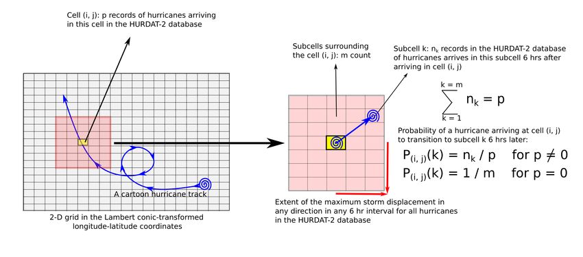
                                                                                                           Fig. 1. Schematic depicting the calculation of displacement probabilities associated with each cell
                                                                                                           in the grid domain.

                                                                                                               It is desirable for the input features to contain information associated with trends of past

                                                                                                                                                            5
______________________________________________________________________________________________________

                                                                                                           storm motion [11, 21]. Once such information is provided by appropriate feature engineer-
                                                                                                           ing, DL methods are well-equipped to excavate complex patterns or relations among input
                                                                                                           and output features that are otherwise intractable. So, storm displacement probabilities
                                                                                                           computed from the historical storms were also included as input features for the current
                                                                                                           model. A schematic depicting the calculation of displacement probabilities is shown in
                 This publication is available free of charge from: https://doi.org/10.6028/NIST.TN.2167

                                                                                                           Fig. 1. At first, the 2 − D domain bounded by the extents of the x− and y− coordinates
                                                                                                           (the extents are the maximum and minimum of each coordinate corresponding to any storm
                                                                                                           record in the considered database) was decomposed into rectangular computational cells.
                                                                                                           Consider all storms for which a record is contained in any one of those computational cells.
                                                                                                           For those storms, the maximum numbers of cells traversed by any storm in any 6 − hr in-
                                                                                                           terval, in the x− and y− directions, are mx and my , respectively. Therefore, associated with
                                                                                                           any given cell (i, j) (colored yellow in Fig. 1) is a set of m = (2mx + 1)(2my + 1) cells
                                                                                                           within which all 6 − hr displacements of any historical storm is contained. Such a set is
                                                                                                           colored red in Fig. 1. Assume there are p records of hurricanes that arrived at the (i, j) −th
                                                                                                           cell and then transitioned to the kth associated cell in the next 6 hours. If this leads to nk
                                                                                                           records being sampled at kth associated cell, ∑m    1 nk = p. Therefore, the displacement prob-
                                                                                                           ability of a storm arriving at the (i, j) − th cell transitioning to the kth associated cell in the
                                                                                                           next 6 hours is,
                                                                                                                                                           (
                                                                                                                                                             nk
                                                                                                                                                                , if p 6= 0
                                                                                                                                              p(i, j) (k) = 1p                                             (3)
                                                                                                                                                             m,    if p = 0
                                                                                                               It is clear that for a fine grid, the number of cells with p = 0 would be larger than for a
                                                                                                           coarse grid. On the other hand, if the grid is too coarse, storm motion trends reflected by
                                                                                                           the displacement probabilities could be obscured. However, for a finer grid (and/ or for a
                                                                                                           very thin upper tail of the distribution of V ), m would increase, and nk would decrease. In
                                                                                                           addition to increased number of features at each instant, displacement probabilities from
                                                                                                           a cell to adjacent cells could be more biased on a specific historical storm’s displacement,
                                                                                                           which is not desirable for the prediction of new storms.

                                                                                                           2.2   Statistics
                                                                                                           The computational domain containing the 1736 storms with at least seven records, includ-
                                                                                                           ing wm , covers intervals of φ ∈ [7.4◦ N, 81◦ N] and λ ∈ [109.5◦W, 63◦ E]. The storm transla-
                                                                                                           tion speeds, which does not exceed V = 40.5 ms−1 for any storm in the database, determines
                                                                                                           the number m of subcells associated with a given computational cell, as shown in Fig. 1.
                                                                                                                Histograms of φ , λ and V have been plotted in Fig. 2. It is evident that for all these
                                                                                                           quantities, the right tail of the distribution is very thin. Only for 33 of the 47880 time
                                                                                                           records was φ > 70◦ N, and only for 26 time records was λ > 10◦ E (to calculate V and
                                                                                                           include it as an input feature, the first time record of the 1736 storms was excluded from the
                                                                                                           dataset). Only 93 records of storm motion satisfied the condition, V > 25 ms−1 . Therefore,
                                                                                                           it is reasonable to exclude the 71 storms for which these limits were exceeded. Thus, 1665
                                                                                                           storms remain in the final database used for model training, validation and testing.

                                                                                                                                                           6
______________________________________________________________________________________________________

                                                                                                                                                                                   8000
                                                                                                                             6000
                                                                                                                                                                                   6000
                                                                                                                 Frequency

                                                                                                                                                                       Frequency
                                                                                                                             4000
                                                                                                                                                                                   4000
                 This publication is available free of charge from: https://doi.org/10.6028/NIST.TN.2167

                                                                                                                             2000                                                  2000

                                                                                                                                0                                                     0
                                                                                                                                    20     40                60   80                      100        50     0    50
                                                                                                                                         Latitude                                                    Longitude
                                                                                                                                                     12000
                                                                                                                                                     10000
                                                                                                                                         Frequency

                                                                                                                                                      8000
                                                                                                                                                      6000
                                                                                                                                                      4000
                                                                                                                                                      2000
                                                                                                                                                         0
                                                                                                                                                             0    10          20          30    40
                                                                                                                                                                               V
                                                                                                           Fig. 2. Histograms of latitude (φ ) and longitude (λ ) in degrees and storm translation speed (V ) in
                                                                                                           ms−1 . Positive values of φ and λ represent the northern and eastern hemispheres, respectively.
                                                                                                           1736 storms from the HURDAT 2 database are used (see text).

                                                                                                               Storm displacement probabilities were calculated based on the evolution of those 1665
                                                                                                           storms. 61 grid points were used in both x and y directions of the LCC projected coordi-
                                                                                                           nates, resulting in the whole 2-D domain being decomposed into 3600 computational cells.
                                                                                                           Despite application of the three above mentioned criteria, 1687 computational cells had
                                                                                                           no time records of an eye of a storm passing through those (i.e., for 1687 out of the 3600
                                                                                                           computational cells, sampled records p = 0). The maximum 6 − hr storm displacement
                                                                                                           in the 1665 storm-database could be captured within mx = my = 4. So, the displacement
                                                                                                           probability was calculated for m = 9 × 9 = 81 associated cells for each computational cell.
                                                                                                           Therefore, the number of input features for each time record was 86 (LCC transformed x
                                                                                                           and y coordinates, storm translation speed V and direction θ , maximum 1 −min wind speed
                                                                                                           at 10 m elevation wm , and historical 6 − hr displacement probabilities calculated at 81 cells
                                                                                                           associated to the cell containing x and y).

                                                                                                           2.3        Zonal data
                                                                                                           Inception locations of the 1665 storms considered for compilation of the database for model
                                                                                                           formulation have been plotted in Fig. 3. The Atlantic basin is generally split into five
                                                                                                           zones or sub-basins, namely, the Tropical Atlantic, the Caribbean sea, Gulf of Mexico,
                                                                                                           East Coast, and Sub-tropical Atlantic. Total storm inceptions in each of these sub-basins

                                                                                                                                                                       7
______________________________________________________________________________________________________

                                                                                                                            Storm inception distribution in each sub-basin
                                                                                                                                                 Sub-basin: Caribbean; St. count: 297;
                                                                                                                                                 Sub-basin: East Coast; St. count: 388;
                 This publication is available free of charge from: https://doi.org/10.6028/NIST.TN.2167

                                                                                                                   30°N                          Sub-basin: Gulf of Mexico; St. count: 279;        50°N
                                                                                                                                                 Sub-basin: Sub-Tropical Atlantic; St. count: 180;
                                                                                                                                                 Sub-basin: Tropical Atlantic; St. count: 521;
                                                                                                                                                                                                   40°N
                                                                                                                   20°N
                                                                                                                                                                                                    30°N
                                                                                                                   10°N
                                                                                                                                                                                                    20°N

                                                                                                                      0°                                                                            10°N

                                                                                                                                                                                                    0°
                                                                                                                      100°W      90°W     80°W     70°W 60°W 50°W 40°W 30°W                  20°W

                                                                                                           Fig. 3. Distribution of storm inception in each sub-basin of the 1665 (out of the 1893) storms from
                                                                                                           the HURDAT2 database used for modeling. Number of storms generated in each sub-basin are
                                                                                                           included.

                                                                                                           are also listed. Figure 4 shows the zonal probability for inception of the historical storms
                                                                                                           considered in Fig. 3. Most of the storm inceptions take place in the tropical region where
                                                                                                           sea-surface termperature is higher. The smallest number of storms are generated farther
                                                                                                           north of latitude 20◦ N in the Sub-Tropical Atlantic.
                                                                                                               Each historical storm’s path-line may be generated by plotting all records from its lifes-
                                                                                                           pan. Each 6 − hr motion of a storm may be approximated as a straight line connecting
                                                                                                           two consecutive records in a storm’s lifespan. In Fig. 5, path-lines of 50 randomly chosen
                                                                                                           storms emerging from each sub-basin are shown. The path-lines are a reasonable represen-
                                                                                                           tation of the underlying trend of storm motion. One might surmise that since the storms
                                                                                                           emerging from a particular sub-basin would be subjected to similar input conditions (e.g.,
                                                                                                           sea surface temperatures), the characterization of their evolution trajectories could be based
                                                                                                           on their inception zones. However, plots in Fig. 5 indicate that a storm’s evolution trend
                                                                                                           is characterized by its instantaneous location. Indeed, the storm tracks show a clear evo-
                                                                                                           lution trend. For example, the overall trend of storms generated in the tropical Atlantic
                                                                                                           sub-basin tend to initially move westward. Then these storms travel northward. Irrespec-
                                                                                                           tive of a storm’s inception zone, north of ≈ 20◦ N, the direction of a storm’s motion slowly

                                                                                                                                                            8
______________________________________________________________________________________________________

                                                                                                                                           0.30
                                                                                                                     St. inception prob.   0.25
                 This publication is available free of charge from: https://doi.org/10.6028/NIST.TN.2167

                                                                                                                                           0.20

                                                                                                                                           0.15

                                                                                                                                           0.10

                                                                                                                                           0.05

                                                                                                                                           0.00
                                                                                                                                                  Trop. At.   Caribbean Gulf of Mexico East Coast Subtrop. At.

                                                                                                           Fig. 4. Zonal storm (St.) inception probability distribution of the 1665 (out of the 1893) storms
                                                                                                           from the HURDAT2 database used for modeling.

                                                                                                           turns eastward. Also, a storm generally moves northward towards regions with colder sea-
                                                                                                           surface temperature. Therefore, training models based on inception sub-basin may not be
                                                                                                           fruitful. As suggested by the plots depicting the storm tracks, an instantaneous location-
                                                                                                           based evolution model that also learns historical storm trajectory trend might work well.
                                                                                                           This work has used DL models that feed on input features such as local coordinates and
                                                                                                           historical displacement probabilities.

                                                                                                                                                                             9
______________________________________________________________________________________________________

                                                                                                                               Sub-basin: Tropical Atlantic;                                          Sub-basin: Caribbean;
                                                                                                              30°N                                                            50°N30°N                                                       50°N

                                                                                                                                                                              40°N                                                           40°N
                                                                                                              20°N                                                                20°N
                 This publication is available free of charge from: https://doi.org/10.6028/NIST.TN.2167

                                                                                                                                                                              30°N                                                           30°N
                                                                                                              10°N                                                                10°N
                                                                                                                                                                              20°N                                                           20°N

                                                                                                                0°                                                            10°N 0°                                                        10°N

                                                                                                                                                                              0°                                                             0°
                                                                                                                100°W   90°W   80°W   70°W 60°W 50°W 40°W 30°W         20°W          100°W   90°W   80°W   70°W 60°W 50°W 40°W 30°W   20°W

                                                                                                                               Sub-basin: Gulf of Mexico;                                             Sub-basin: East Coast;
                                                                                                              30°N                                                            50°N30°N                                                       50°N

                                                                                                                                                                              40°N                                                           40°N
                                                                                                              20°N                                                                20°N
                                                                                                                                                                              30°N                                                           30°N
                                                                                                              10°N                                                                10°N
                                                                                                                                                                              20°N                                                           20°N

                                                                                                                0°                                                            10°N 0°                                                        10°N

                                                                                                                                                                              0°                                                             0°
                                                                                                                100°W   90°W   80°W   70°W 60°W 50°W 40°W 30°W         20°W          100°W   90°W   80°W   70°W 60°W 50°W 40°W 30°W   20°W

                                                                                                                                                              Sub-basin: Sub-Tropical Atlantic;
                                                                                                                                             30°N                                                                 50°N

                                                                                                                                                                                                                  40°N
                                                                                                                                             20°N
                                                                                                                                                                                                                  30°N
                                                                                                                                             10°N
                                                                                                                                                                                                                  20°N

                                                                                                                                               0°                                                                 10°N

                                                                                                                                                                                                                  0°
                                                                                                                                               100°W   90°W     80°W   70°W 60°W 50°W 40°W 30°W            20°W

                                                                                                           Fig. 5. 50 randomly selected historical storm tracks from HURDAT2 plotted based on their
                                                                                                           inception sub-basins. Trajectory between two consecutive records in 6 − hr intervals in a storm’s
                                                                                                           lifetime has been approximated as a straight line.

                                                                                                                                                                                   10
______________________________________________________________________________________________________

                                                                                                           3.     Model development

                                                                                                           Once a database was obtained, we proceeded to the model development. Both classifica-
                                                                                                           tion and regression problems may be formulated. In the current work, for either of these
                                                                                                           problems, we used the Long short-term memory (LSTM) [10] Recurrent Neural Networks
                 This publication is available free of charge from: https://doi.org/10.6028/NIST.TN.2167

                                                                                                           (RNN). This section considers the formulation of the current problem with the chosen RNN
                                                                                                           model and its implementation, including model training and model parameter tuning.

                                                                                                           3.1     Classification

                                                                                                                          Hurr. Andrew, 1992                                           Hurr. Ivan, 2004
                                                                                                                                Truth                                                      Truth
                                                                                                           30°N                 Interpolated; avg. err. 50.02 mi 50°N 30°N                 Interpolated; avg. err. 54.25 mi 50°N

                                                                                                                                                                40°N                                                       40°N
                                                                                                           20°N                                                        20°N
                                                                                                                                                                30°N                                                       30°N
                                                                                                           10°N                                                        10°N
                                                                                                                                                                20°N                                                       20°N
                                                                                                             0°                                                 10°N     0°                                                10°N

                                                                                                                                                         0°                                                          0°
                                                                                                            100°W 90°W 80°W 70°W 60°W 50°W 40°W 30°W 20°W               100°W 90°W 80°W 70°W 60°W 50°W 40°W 30°W 20°W
                                                                                                                           Hurr. Sandy, 2012                                          Hurr. Harvey, 2017
                                                                                                                                Truth                                                      Truth
                                                                                                           30°N                 Interpolated; avg. err. 51.65 mi 50°N 30°N                 Interpolated; avg. err. 52.68 mi 50°N

                                                                                                                                                                40°N                                                       40°N
                                                                                                           20°N                                                        20°N
                                                                                                                                                                30°N                                                       30°N
                                                                                                           10°N                                                        10°N
                                                                                                                                                                20°N                                                       20°N
                                                                                                             0°                                                 10°N     0°                                                10°N

                                                                                                                                                         0°                                                          0°
                                                                                                            100°W 90°W 80°W 70°W 60°W 50°W 40°W 30°W 20°W               100°W 90°W 80°W 70°W 60°W 50°W 40°W 30°W 20°W

                                                                                                           Fig. 6. Interpolation error of selected hurricane trajectories; actual trajectories are colored red, and
                                                                                                           the blue symbols represent the actual coordinates interpolated to the center of the 2 − D
                                                                                                           computational cell containing it. Error in miles averaged over the whole trajectory is given.

                                                                                                               A classification problem may be envisaged utilizing the structured computational grid
                                                                                                           for the calculation of 6 − hr storm displacement probabilities. Given a storm’s current
                                                                                                           location, translation velocity and 6 − hr displacement probabilities, the model could be
                                                                                                           trained on predicting the subcell number k in Fig. 1. In that case, the training and testing
                                                                                                           data targets would be the One-Hot encoded subcell number k, to which a storm eye located
                                                                                                           within a given computational cell at a given instant transitions in the next time instant.

                                                                                                                                                                       11
______________________________________________________________________________________________________

                                                                                                           Generally, DL algorithms are trained to assign a probability to each class in a classification
                                                                                                           problem. In the current problem, probabilities will be assigned to each of the m = 81
                                                                                                           subcells associated with a computational cell. From a computational cell (i, j), a storm
                                                                                                           moves to the subcell for which the assigned probability is maximum. The storm location at
                                                                                                           the next time instant is calculated from the k − th associated cell’s location relative to the
                 This publication is available free of charge from: https://doi.org/10.6028/NIST.TN.2167

                                                                                                           computational cell (i, j). The storm eye is interpolated to the center of the k −th associated
                                                                                                           cell containing it.
                                                                                                               Selected hurricane trajectories are shown in Fig. 6. In addition to the actual 6 − hr
                                                                                                           hurricane eye positions in the database (marked by red symbols), the positions obtained by
                                                                                                           interpolation to the center of the computational cells containing these are also shown. Er-
                                                                                                           ror in miles averaged over the whole trajectory of each hurricane have been reported. The
                                                                                                           computational grid (as in Fig. 1) used for this purpose contains 60 cells in each of longitude
                                                                                                           and latitude directions. The number of subcells associated with each computational cell is
                                                                                                           143 (13 × 11) and is used for displacement probability calculations as well as for predic-
                                                                                                           tion of classes for the classification problem on storm trajectory evolution. The averaged
                                                                                                           interpolation error in miles is ≈ 80.5 km (50 mi) for each location for all hurricanes. Due
                                                                                                           to the interpolation error alone, the predictions are likely to veer off the actual trajectories
                                                                                                           very quickly. As this error is more than the average forecasting error obtained from the
                                                                                                           regression problem, the classification approach was not pursued.

                                                                                                           3.2   Regression
                                                                                                           The supervised regression problem under consideration is relatively straightforward. The
                                                                                                           inputs to the model are the two LCC projected x– and y–coordinates, storm translation ve-
                                                                                                           locity (speed V and direction θ ), max. 1–min windspeed at a 10 m elevation wm , and 6–hr
                                                                                                           storm displacement probabilities associated with the storm’s position in the computational
                                                                                                           grid at the current and few previous timesteps (86 input features at each timestep × the
                                                                                                           number of timesteps). The model outputs are the storm position(s) x and y at 6 − hr in-
                                                                                                           tervals for the chosen number of output timesteps. The model performance, measured in
                                                                                                           the classification problem in terms of accuracy, is measured by the loss function defined as
                                                                                                           the mean squared error (m.s.e.) between the model predicted and the true position(s) of N
                                                                                                           samples.

                                                                                                                                     ∑N                               2
                                                                                                                                        i=1 (x predicted,i − xtrue,i ) + (y predicted,i − ytrue,i )
                                                                                                                                                                                                   2
                                                                                                                           m.s.e. =
                                                                                                                                                                     N
                                                                                                               Gradients of the m.s.e. are computed w.r.t. changes in parameters/ weights of the model.
                                                                                                           The model weights are updated so that the m.s.e. is minimized. V , θ and 6 − hr displace-
                                                                                                           ment probabilities associated with each timestep are computed from the storm’s position at
                                                                                                           the current and previous timesteps. These features are used as inputs in the next timestep.
                                                                                                           For the current purpose of predicting the storm trajectories, true values of wm are used at
                                                                                                           each timestep for model testing.

                                                                                                                                                         12
______________________________________________________________________________________________________

                                                                                                           3.3    Model: LSTM RNN
                                                                                                           Recurrent Neural Networks (RNN) were innovated to extract pattern and context from se-
                                                                                                           quences. RNNs are applied in a wide range of sequence related problems, including mod-
                                                                                                           eling and prediction of languages and sentiment, video tagging, a sequence prediction in
                 This publication is available free of charge from: https://doi.org/10.6028/NIST.TN.2167

                                                                                                           time. HURDAT2 is a sequence of time records. RNNs may therefore be expected to be
                                                                                                           useful for predicting evolving dynamical systems that depend on events of the past, such
                                                                                                           as hurricanes [7, 12]. Among all RNN algorithms, Long Short-Term Memory (RNN) algo-
                                                                                                           rithm was prescribed in [10] to tackle the vanishing gradient problem. Over long sequences,
                                                                                                           relevant past information may get lost or, equivalently, gradients may vanish while training
                                                                                                           a model using back propagation. In an LSTM unit, past information may be retained via a
                                                                                                           cell state that passes through all LSTM layers. Early use of LSTMs in weather forecasting
                                                                                                           is reported in [22].

                                                                                                                          Fig. 7. Different LST M RNN architectures used in the present study.

                                                                                                                 Schematics of the LSTM RNN models used in the present work have been shown in

                                                                                                                                                          13
______________________________________________________________________________________________________

                                                                                                           Fig. 7. In the figures, the vector represented by ~xi contains the input features at the ith time
                                                                                                           instant. The input layer is colored yellow. For Many-To-One algorithms (M2O) n–time
                                                                                                           records are fed to the model to obtain the output vector ~h in the output layer (green). One
                                                                                                           or several layers of LSTM-RNN units (blue) may be used. Increased depth of the net-
                                                                                                           works augments their ability to learn complex patterns. The M2O model results presented
                 This publication is available free of charge from: https://doi.org/10.6028/NIST.TN.2167

                                                                                                           here used 3 layers of LSTM units. Many-To-Many (M2M) prediction models used here
                                                                                                           output the same number of time records (~hi ’s) as the number of input time records (n in
                                                                                                           the diagram). Bi-Directional LSTM layers were used for the M2M LSTM model. Each
                                                                                                           bi-directional layer comprises two layers of LSTMs receiving the inputs separately in an
                                                                                                           ascending and a descending order in time, respectively. Some information from the future
                                                                                                           may thus be used to predict an earlier timestep.

                                                                                                           Fig. 8. A representative LSTM unit; the unit belongs to the qth layer of the model. Corresponding
                                                                                                           input time step is n, i.e., at the input layer (q = 1), h~0n = x~n input features at the nth timestep. The
                                                                                                           symbols × and + represent pointwise operation.

                                                                                                               An LSTM unit/ cell is shown in Fig. 8. The superscript in the vector variables indi-
                                                                                                           cates the layer number (this unit belongs to layer q of the model); the subscript denotes the
                                                                                                           corresponding input step n as in Fig. 7. A cell comprises four main components, the cell
                                                                                                           state (passing through the units, colored red), the forget gate (colored orange), the input
                                                                                                           gate (colored green) and the output gate (colored blue). The three gates basically apply the
                                                                                                           three activation functions (in the schematic, σ and tanh represent sigmoid and hyperbolic
                                                                                                           tangent activation functions, respectively), each of which has a specific role in informa-

                                                                                                                                                               14
______________________________________________________________________________________________________

                                                                                                                                                                    −−→
                                                                                                                                                                      (q)
                                                                                                           tion propagation through the model. The cell state (Cn ) is the unique component of an
                                                                                                           LSTM RNN. The cell state passes through all timesteps n = 1, 2, ... of a given layer, and is
                                                                                                           therefore able to preserve information from the past and also accumulate new information
                                                                                                           with increasing n [23]. The cell shown in the diagram receives an input from the previous
                                                                                                                                                    −−−→
                 This publication is available free of charge from: https://doi.org/10.6028/NIST.TN.2167

                                                                                                                                                     (q−1)
                                                                                                           layer belonging to the same time step hn        , and also from the previous time step in the
                                                                                                                         −−→
                                                                                                                           (q)
                                                                                                           same layer, hn−1 . Based on these inputs to the cell, the forget gate dictates the part of the
                                                                                                           cell state to be discarded at the current unit. On the basis of these same inputs, input gate
                                                                                                           dictates the information from the present inputs to be added (marked by +) to the cell state.
                                                                                                           Consequently, after these operations, the cell state gets modified in the current LSTM unit
                                                                                                            −−→ −−→
                                                                                                              (q)       (q)
                                                                                                           (Cn−1 → Cn ), which is the cell state received by the LSTM cell to the right, i.e., the next
                                                                                                           timestep in the same layer. The updated cell state also participates in obtaining the output
                                                                                                                                   −→
                                                                                                                                    (q)
                                                                                                           from the current cell (hn ) after the sigmoid activation is applied at the output gate.

                                                                                                           3.4              Model: Architecture & Implementation
                                                                                                           Models trained on varying numbers of input time records (n) can predict one or several time
                                                                                                           steps at once based on their architecture. Both Many-To-One (M2O) and Many-To-Many
                                                                                                           (M2M) type prediction algorithms have been used. As their nomenclature suggests, upon
                                                                                                           processing a time sequence with n time records, the M2O prediction models forecast the
                                                                                                           storm locations at only one time instant, while the M2M models used here output n number
                                                                                                           of time records. From here onwards, models are named as M2On or M2Mn to reflect their
                                                                                                           architecture. As each timestep in the training database ≡ 6 − hr, the M2On and M2Mn
                                                                                                           models forecast 6 and 6n hours at once, respectively.

                                                                                                                                            Model error reduction: Input time records 3                              Model error reduction: Input time records 3
                                                                                                                                   10   1
                                                                                                                                                                       No. of layers 1                                                          No. of layers 1
                                                                                                                                   10   2
                                                                                                                                                                       No. of layers 2                      10   2                              No. of layers 2
                                                                                                                                                                       No. of layers 3                                                          No. of layers 3
                                                                                                                 Training m.s.e.

                                                                                                                                                                                          Training m.s.e.

                                                                                                                                                                       No. of layers 4                      10   3
                                                                                                                                                                                                                                                No. of layers 4
                                                                                                                                   10   3
                                                                                                                                                                       No. of layers 5                                                          No. of layers 5
                                                                                                                                   10   4                                                                   10   4

                                                                                                                                   10   5                                                                   10   5

                                                                                                                                            100            101            102                                        100            101            102
                                                                                                                                                                 epochs                                                                   epochs
                                                                                                           Fig. 9. Training loss plotted against epochs for different number of hidden LSTM-RNN layers in
                                                                                                           the M2O prediction models with similar (different) number of trainable parmaters in each model
                                                                                                           shown in the left (right) frame.

                                                                                                           Hidden layers: The number of hidden layers is an important model parameter. Theoreti-
                                                                                                           cally, a model is able to capture more complex patterns in the underlying data with increase

                                                                                                                                                                                          15
______________________________________________________________________________________________________

                                                                                                           in number of hidden layers/ model depth. However, increasing the number of layers will
                                                                                                           increase the number of trainable parameters, possibly resulting in data overfitting. In a set
                                                                                                           of simulations with up to 5 hidden layers for the M2O LSTM-RNNs, the layer-to-layer
                                                                                                           output dimension was reduced with increasing depth in the model, so that the number of
                                                                                                           trainable parameters did not change significantly among the models with additional hidden
                 This publication is available free of charge from: https://doi.org/10.6028/NIST.TN.2167

                                                                                                           layers. In another set of simulations, the layer-to-layer output dimension was kept constant
                                                                                                           in the hidden LSTM layers, so that the number of trainable parameters was proportional to
                                                                                                           the number of hidden layers. The number of trainable parameters represents the degrees-
                                                                                                           of-freedom for a model. The number of input time records was also varied. In Fig. 9,
                                                                                                           reduction of the loss function defined as the mean-squared-error (m.s.e.) between the pre-
                                                                                                           dicted and true scaled LCC coordinates, is plotted against the number of epochs. The left
                                                                                                           frame shows the error reduction for models with similar numbers of trainable parameters;
                                                                                                           the right frame shows the same plot for models with various numbers of trainable parame-
                                                                                                           ters. For both sets of models the error level saturates at around the same value after about
                                                                                                           200 epochs. The performance of models after convergence does not improve with addi-
                                                                                                           tional LSTM layers in either plot. Similar performance was also obtained for models (not
                                                                                                           shown here) that feed on more or less than 3 input time records.
                                                                                                               Increasing hidden RNN layers may result in an increase in the number of trainable pa-
                                                                                                           rameters. To avoid overfitting the training data, approximately similar numbers of trainable
                                                                                                           parameters were used when checking for optimal numbers of layers for both M2O and
                                                                                                           M2M models. In addition to the input and output layers, three layers of LSTM-RNN cells
                                                                                                           were used for the final version of the M2O LSTM model. It was found that increasing
                                                                                                           the number of hidden LSTM layers while keeping the number of trainable parameters ap-
                                                                                                           proximately the same did not improve the results significantly. The numbers of neurons
                                                                                                           in the three hidden LSTM layers between the input and output layers were 128, 32 and 8,
                                                                                                           respectively.
                                                                                                               For the M2M models, two bi-directional LSTM layers were used at either side of a
                                                                                                           repeat-vector layer. This layer is required for the multi-step data transfers between two
                                                                                                           layers and does not contain any trainable parameter. Before the output layer, a time-
                                                                                                           distribution layer was required to output multiple time steps. Each of the LSTM cells
                                                                                                           in bi-directional layers had an input and output dimension of 64; a total of 128 neurons
                                                                                                           were used in each of these layers. The number of trainable parameters for all the tested
                                                                                                           models were between 3 to 6 times the numbers of data sequences/ samples obtained from
                                                                                                           the database.
                                                                                                           Dropout: To increase the robustness of NN models, a regularization parameter called
                                                                                                           dropout is used. This value indicates the number of randomly chosen neurons to be switched
                                                                                                           off in each layer. Dropping out neurons increases variance in model prediction while re-
                                                                                                           ducing the model’s bias towards the training data. For this reason the important dropout pa-
                                                                                                           rameter is widely used to avoid overfitting. We used a dropout value of 0.1 for each hidden
                                                                                                           layer, meaning that 10 % of the neurons were randomly dropped at each hidden layer
                                                                                                           when feeding the data forward from layer to layer. Special care was taken in considering
                                                                                                           the number of trainable parameters for each model. Tuning the dropout value to increase

                                                                                                                                                        16
______________________________________________________________________________________________________

                                                                                                           model robustness was deemed unnecessary.
                                                                                                           Optimization: The models were trained with the Adam optimization algorithm [24]. The
                                                                                                           algorithm updates the weights of the NNs via backpropagation based on the loss functions
                                                                                                           calculated in the current epoch or the optimization iteration loop. Finally, the models were
                                                                                                           implemented using the Keras API. Keras is a popular high-level NN framework written in
                 This publication is available free of charge from: https://doi.org/10.6028/NIST.TN.2167

                                                                                                           Python. It can use several lower-level APIs as chosen by the user. We used the Keras API
                                                                                                           with TensorFlow as the lower level backend library.

                                                                                                           3.5   Model: Training strategies
                                                                                                           Number of input time records (n): Several aspects of model training and validation war-
                                                                                                           rant discussion due to the complexity of the problem under consideration. An important
                                                                                                           consideration is the number of input time instants, n that could minimize the model pre-
                                                                                                           diction error. Intuitively, increase in n should make the model prediction more accurate.
                                                                                                           However, a high value of n implies that the predictions may only be obtained when the
                                                                                                           storm has significantly evolved. Consequently less time is available for preparation of a
                                                                                                           possible landfall, which is undesirable. This choice also dictates model training strategy.
                                                                                                           Number of input time records used in each input sequence implicitly determines the num-
                                                                                                           ber of data sequences that may be generated from the storm database for model training/
                                                                                                           validation/ testing. Additional preprocessing such as zero padding may be used at early
                                                                                                           stages of a storm’s life span (available time instants < n). To mitigate this issue, both
                                                                                                           M2On and M2Mn LSTM models were developed for a range of n, between 1 and up to 5
                                                                                                           time instants (nmax = 5 in Fig. 7).
                                                                                                           Data scaling: Scaling of the data fed to the neural networks is an important aspect of
                                                                                                           the present problem. NNs perform better when the input data is contained in the interval
                                                                                                           [0, 1]. Note that each storm in the database is an individual entity that may be totally
                                                                                                           uncorrelated with some or most other storms. Also, the total distance traveled by any storm
                                                                                                           in the database should be proportional to the number of available records for that storm.
                                                                                                           This has led other researchers [12] to use storm-based scaling, so that the features for any
                                                                                                           storm contains both upper (1) and lower (0) bounds. In this work data normalization for the
                                                                                                           whole database under consideration was performed using the Min-Max scaler. Each feature
                                                                                                                                   f − fmin
                                                                                                            f is scaled as, fs = fmax − fmin , so that scaled feature f s is contained in the interval [0, 1].
                                                                                                           This scaling is preferred over standardization, because the displacement probabilities also
                                                                                                           belong in this interval. Furthermore, to predict a new storm’s evolution using the trained
                                                                                                           model, scaling of the features is well defined as the maximum and minimum of a feature
                                                                                                           are taken from the database on which the model is trained and validated. The storm-wise
                                                                                                           data scaling method renders prediction of a new storm impossible, because the relevant
                                                                                                           scaling parameters such as the minimum, maximum or the mean and standard deviation of
                                                                                                           a feature for a new storm are unknown a priori.
                                                                                                           Sequence generation: Although whole database scaling was preferred over storm-wise
                                                                                                           data scaling, storms were segregated for the purpose of training, validation and testing.
                                                                                                           A few important historical storms were chosen for testing. The rest of the storms were

                                                                                                                                                           17
______________________________________________________________________________________________________

                                                                                                           chosen randomly from the database without replacement. Of the 1665 storms considered,
                                                                                                           1332 (i.e., ≈ 80%) were used for training the model while 15% storms were used for vali-
                                                                                                           dation. Data sequences for training, validation and testing were generated separately from
                                                                                                           the segregated lists of storms. The number of sequences used for training, validation and
                                                                                                           testing varied between specific training instances because of random sampling of storms
                 This publication is available free of charge from: https://doi.org/10.6028/NIST.TN.2167

                                                                                                           and also because lifespans of storms vary. The number of training data sequences was
                                                                                                           always ∼ 30, 000 or more. In some earlier works [11, 12], a portion of a given storm’s
                                                                                                           data was used for training. The model was tested on the remaining portion of the storm’s
                                                                                                           records. In our view, this provides an unfair test of the model performance, owing to bias
                                                                                                           associated with prediction on a storm, some portion of which has been already seen by
                                                                                                           the model. A trained model would not have this advantage for real-time forecasting of an
                                                                                                           entirely new storm absent in the database.

                                                                                                           3.6   Hyperparameter tuning
                                                                                                           While training a NN, several user defined parameters must be tuned to obtain best per-
                                                                                                           formance. These are often chosen manually and tuned by trial and error. The important
                                                                                                           hyperparameters chosen via tuning, the learning rate, the number of full optimization iter-
                                                                                                           ations/ epochs the model is subjected to and the batch size are discussed here.
                                                                                                           Learning rate & Epochs: The learning rate is a hyperparameter of the optimizer algo-
                                                                                                           rithm which indicates the rate of updating of weights w.r.t. the computed deviation of the
                                                                                                           loss function for small changes in weights. A high learning rate converges to the optimal
                                                                                                           weights faster while a small learning rate may require a large number of epochs to con-
                                                                                                           verge. However, a large learning rate may result in missing the optimal point. In Keras, the
                                                                                                           default learning rate for the Adam optimizer is set as 0.001. At this default value, the vali-
                                                                                                           dation loss was prone to sudden jumps in and around the optimal valley’s minimum. In our
                                                                                                           calculations, to smoothly converge to the optimal weights we used an initial learning rate
                                                                                                           of 0.0001 for the first 250 epochs. Each epoch represents a full model-weight optimization
                                                                                                           loop including a forward pass of calculating the predictions based on all the input sequences
                                                                                                           from the training data and a backpropagation step, in which the model weigths are updated
                                                                                                           based on the calculated loss function in the forward step. In the subsequent training itera-
                                                                                                           tions, models already trained were further trained by reducing the learning rate by an order
                                                                                                           of magnitude every 250 epochs (for example, for the second set of 250 epochs the learning
                                                                                                           rate was 0.00001). This is done until the models stop improving.
                                                                                                           Batch size: Another important hyperparameter for efficient model training is the batch size.
                                                                                                           In each epoch, all training time sequences are subjected to the forward model prediction
                                                                                                           pass once. However, for quicker model convergence, a smaller number of sequences may
                                                                                                           be used at a time for an optimization loop and model parameters/ weights may be updated.
                                                                                                           This can be done several times within an epoch. The smaller number of sequences used
                                                                                                           for updating the model weights one time in each of these sub-epochs is called the batch
                                                                                                           size. Too large batch size results in smooth gradients computed and averaged over all input
                                                                                                           sequences. On the other hand, small batch size results in chaotic gradient calculations as-

                                                                                                                                                        18
______________________________________________________________________________________________________

                                                                                                           sociated with properties of small chunks of training data sequences resulting in an irregular
                                                                                                           path to converged solutions. In our calculations, we used a batch size of 32 which signif-
                                                                                                           icantly quickened the training process, especially in the Graphic Processing Unit (GPU)
                                                                                                           clusters. A checking criterion/ checkpoint for model performance was used to check model
                                                                                                           performance after completion of each epoch. The model weigths were stored in case the
                 This publication is available free of charge from: https://doi.org/10.6028/NIST.TN.2167

                                                                                                           validation loss obtained with the updated model weights was lower than the validation loss
                                                                                                           obtained with the previously stored model weights. At the end of the entire training pro-
                                                                                                           cess, model weights were thus obtained that yielded the lowest loss function value defined
                                                                                                           by the m.s.e. between the predicted and the true LCC coordinates for the validation data
                                                                                                           sequences.

                                                                                                                                                        19
______________________________________________________________________________________________________

                                                                                                           4.    Results

                                                                                                           In the following discussion, models are named to reflect their prediction architecture. These
                                                                                                           models have been named M2On and M2Mn, where, n = 1, 2, 3, 4 and 5 represents the
                                                                                                           number of records a model takes in as input. As each timestep in the training database
                 This publication is available free of charge from: https://doi.org/10.6028/NIST.TN.2167

                                                                                                           ≡ 6 − hr, the M2On and M2Mn models forecast 6 and 6n hours at once, respectively.

                                                                                                           4.1      Mean forecast error
                                                                                                           A set of five historical storms were always included in the test dataset. These five storms
                                                                                                           were chosen on account of their destructiveness upon landfall and of the complexity of their
                                                                                                           trajectories. The other storms were randomly chosen without replacement for validation
                                                                                                           and testing. 15% of the storms from the eventual 1665–storm database were chosen for
                                                                                                           validation purposes and 5% as test storms. Once the models were trained, these were tested
                                                                                                           on both the validation and test storms. The average error in distance between the predicted
                                                                                                           and the true positions of a storm’s eye was computed at each prediction step.
                                                                                                                               (a)                                                           (b)
                                                                                                                              45                                         45                 45                                         45

                                                                                                                              40                               M2O       40                 40                               M2O       40
                                                                                                                                                               M2M                                                           M2M
                                                                                                                 error (km)

                                                                                                                                                                               error (km)

                                                                                                                              35                                         35                 35                                         35

                                                                                                                              30                                         30                 30                                         30

                                                                                                                              25                                         25                 25                                         25
                                                                                                                                   1   2         3         4         5                           1   2         3         4         5
                                                                                                                                       input time records (n)                                        input time records (n)

                                                                                                           Fig. 10. Average 6–hr forecasting error in distance for the M2O and M2M models computed on (a)
                                                                                                           validation and (b) test storms.

                                                                                                               Average 6 − hr forecast error in distance for all models is shown in Fig. 10. The plots in
                                                                                                           Fig. 10(a) and 10(b) show the average error computed on the validation and test sequences,
                                                                                                           respectively. Figure 10 demonstrates that the models have been optimally trained as the
                                                                                                           validation and test errors are very similar for all models. Overall, the M2M models are more
                                                                                                           accurate for all n. The M2M2 model performs best of all models for 6 − hr forecasting;
                                                                                                           mean error computed for the validation and test storms are 34.2 and 30 km, respectively.
                                                                                                           This is not surprising: authors in [19] noted a near linear statistical relationship between
                                                                                                           time-rate changes in translation variables at current and previous timesteps, meaning that
                                                                                                           storm velocity information from two previous instants is likely to produce a more accurate
                                                                                                           prediction. Although the number of trainable parameters for all models belong in a similar
                                                                                                           range, the M2On models improve with increase in n, and the M2Mn model predictions
                                                                                                           worsen slightly with increase in n > 2. This is because the M2M models predict several

                                                                                                                                                                              20
You can also read