A Walking Velocity Update Technique for Pedestrian Dead-Reckoning Applications
←
→
Page content transcription
If your browser does not render page correctly, please read the page content below
A Walking Velocity Update Technique for
             Pedestrian Dead-Reckoning Applications
                                 Chi-Chung Lo∗ , Chen-Pin Chiu∗ , Yu-Chee Tseng ∗ ,
                                         Sheng-An Chang†, and Lun-Chia Kuo†
             ∗ Department of Computer Science, National Chiao-Tung University, Hsin-Chu 300, Taiwan
                          † Industrial Technology Research Institute, Hsin-Chu 310, Taiwan

              Email: {ccluo, cpchiu, yctseng}@cs.nctu.edu.tw; {changshengan, jeremykuo}@itri.org.tw

   Abstract—Inertial sensors for pedestrian dead-reckoning            the user’s ankle. Empirical evidence supports the claim that
(PDR) have been attracting considerable attention recently. Since     angular rate data is more reliable than acceleration data. In
accelerometers are prone to the accumulation of errors, a “Zero       [14], regression analysis was used to detect walking frequency
Velocity Update” (Z-UPT) technique [1], [2] was proposed as a
means to calibrate the velocity of pedestrians. However, these        and the variance in signals from an accelerometer during a
inertial sensors must be mounted on the bottom of the foot,           single step, from which a conversion equation between stride
resulting in excessive vibration and errors when measuring            length and step duration was derived. Nonetheless, each of
speed or orientation. This paper proposes a self-calibrating PDR      these systems produce a high degree of error when users
solution using two inertial sensors in conjunction with a novel       deviate from their normal walking patterns.
concept called “Walking Velocity Update” (W-UPT). One inertial
sensor is mounted on the lower leg to identify a point suitable for      A fundamental issue in reducing measurement error in PDR
calibrating the walking velocity of the user (when its pitch value    systems is identifying the most effective method with which
becomes zero), while another sensor is mounted on the upper           to calibrate the system. This is primarily due to the fact
body to track the velocity and orientation. We have developed a       that accelerometers tend to accumulate a considerable number
working prototype and tested the proposed system using actual         of errors when data is converted to speed or displacement.
data.
                                                                      To overcome error drifting problems, a technique known as
Keywords: body sensing, inertial measurement unit, location
                                                                      Z-UPT (Zero Velocity Update) employing a foot-mounted
tracking, pedestrian dead-reckoning, wireless sensor network.
                                                                      inertial sensor was proposed [1], [2]. Readings taken by these
                                                                      sensors are reported to be very close to zero when the sole of
                       I. I NTRODUCTION
                                                                      the foot touches the ground. This event represents a suitable
   A large number of location-based services (LBS) [3], [4],          moment from which to calibrate the system, i.e., the velocity
such as navigation and tracking, have recently been proposed,         of the walker is reset to zero when the system detects the
and a central issue in all such applications is location tracking.    occurrence of such an event. The main drawback of Z-UPT
Currently, GPS remains the most widely used technology                is that the inertial sensor must be mounted on the bottom
for positioning in outdoor environments; however, due to              of the foot, leading to excessive vibration and error in the
shadowing effects, GPS is not always available or reliable.           measurement of orientation and displacement.
To overcome these limitations, considerable effort has been              Our objective in this study was to develop an approach to
dedicated to the development of alternative positioning tech-         eliminate both accumulated and orientation based errors. We
niques. These techniques can be classified into six categories:       propose a novel concept called “Walking Velocity Update”
AoA-based [5], ToA-based [6], TDoA-based [7], signal loss-            (W-UPT), using an inertial sensor mounted on the lower
based [8], pattern-matching [9], [10], [11], and pedestrian           leg and a second sensor on the upper body. The lower
dead-reckoning [1], [2], [12], [13], [14] techniques.                 sensor determines the timing aspect of walking velocity and
   This work focuses primarily on PDR systems that rely on            continuously forwards this information to the upper sensor.
inertial sensors, such as accelerometers, electronic compasses,       The upper sensor calculates the velocity of the user according
and gyro sensors mounted on the human body. These devices             to measurements of acceleration calibrated against data from
are used to measure acceleration, orientation, and angles of          the lower sensor. The upper sensor also provides information
rotation to track the location of users. The simplest PDR             related to the orientation of the user. Our results are based on
system is the pedometer, which counts steps; however, walking         the following observations concerning walking motion. First,
motion actually comprises of a series of strides, which are           the angular velocity of the lower leg with respect to the ground
far more effectively characterized by triaxial accelerometers         can be used to determine the walking velocity of an individual
and e-compass sensors. In [12], a pattern matching method             when the thigh and lower leg form a straight line. Second,
was used to derive strides from vertical accelerations. In [13],      when the aforementioned straight line is perpendicular to the
step events were detected through the cooperative efforts of          ground (i.e., its pitch value = 0), the angular speed can be
a vertical accelerometer and the angular rate at the axis of          accurately converted to body speed. Third, for the purpose of
Inertial Sensor
Hip joint
Ankle joint
{
Rigid Body
Walking Velocity v
Tangential Velocity v
L
Angular Velocity
Fig. 1. System model of of W-UPT.
(a)
Acceleration and Inertial Sensor
Orientation
Raw Data
Sb Walking
Processing
Velocity
v'
Update Location
Straight-line Tracking
Pitch Condition
Sl Raw Data 50°
Processing Stride
Stride
Detection
Event 0°
-50°
Fig. 2. Workflow of the W-UPT method.
(b)
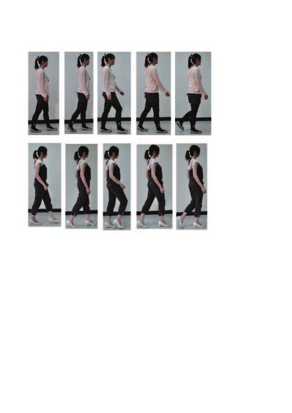
Fig. 3. (a) Five poses of a stride from two users and; (b) walking posture
trajectory tracking, mounting an inertial sensor on the upper versus pitch angles.
body incurs fewer positioning errors than mounting one on the
lower leg. A prototype was developed to verify these claims.
The remainder of this paper is organized as follows. A the thigh and lower leg gradually form a straight line, which
model of the proposed system is presented in Section II. we call the straight-line condition. When this condition is met,
A number of implementations and experimental results are the horizontal component of the tangential velocity over the
presented in Section III. Conclusions are drawn in Section IV. hip joint is equal to that of the body (because at this point they
merge into a single rigid entity). Let L be the length of the
II. S YSTEM M ODEL leg, v be the velocity of the upper body, v 0 be the tangential
An inherent limitation of most PDR solutions is the problem velocity of the hip joint, and ω be the angular velocity of the
of error drifting. Z-UPT deal with this problem by resetting lower leg. According to Newton’s Second Law, we assume that
the velocity of the user to zero, when it detects slippage of the following equality holds when the thigh and the lower leg
the sole on the floor. This approach requires that the sensor from a straight line:
be mounted on the bottom of the foot, which inevitably
v 0 = ω × L. (1)
leads to excessive vibration and error in the measurement
of orientation. To alleviate this problem, we propose a W- Note the tangential velocity and the angular velocity only refer
UPT solution, involving the use of two inertial sensors Sl to their magnitudes (i.e., no direction is involved). Because L
and Sb mounted on the lower leg and upper body of the is given and ω can be measured by Sl , it is possible to derive
user, respectively. Sb measures the velocity of the user and v 0 . The projection of v 0 on the ground is equal to v. It follows
is re-calibrated every stride according to the angular velocity that when the pitch value is zero, we have
measured by Sl .
v = v0 . (2)
Our system model is shown in Figure 1. Sensor Sb is
attached to the user’s upper body and sensor Sl attached to the Therefore, we use v 0 to calibrate the value of v measured by
user’s lower leg. In every stride, the sole touches the ground Sb when the pitch value of Sl is zero for every stride. (Note
for a short period of time. During this period, we observe that that v is indirectly derived by the accelerometer of Sb .)55 mm
Inertial sensor on
upper body
ZigBee
28 mm
ZigBee Inertial sensor on
13 mm low leg
Inertial Sensor
(a) (b)
Fig. 4. (a) Inertial sensor; (b) sensors mounted on the upper body and the lower leg.
Figure 2 shows the workflow of W-UPT. Sb comprises value of ω, a number of filtering techniques may be used. In
a triaxial accelerometer, a triaxial e-compass, and a triaxial this case, we adopted a Low-Pass filter [15] to achieve this
gyro sensor. Sl consists of a triaxial e-compass and a triaxial goal.
gyro sensor. The Raw Data Processing block for Sb extracts
information related to acceleration and orientation from the C. Location Tracking Block
sensing data of Sb . The Raw Data Processing block for Sl
extracts pitch and angular velocity ω from the sensing data When a stride event is reported to the Location Tracking
of Sl . The Stride Detection block uses pitch to identify two block, it begins computation of the length and direction of the
events: stride events and straight-line conditions. Upon the following stride, by integrating the acceleration and orientation
occurrence of a straight-line condition, the Walking Velocity of Sb during the current stride, until the next stride event is
Update block computes current v 0 and report this velocity to reported. Let at be the acceleration measured by Sb at time t,
the Location Tracking block. The Location Tracking block ti be the time when the ith stride is reported, and ti+1 be the
then calibrates its v as v 0 and computes the length and direction time when the (i + 1)th stride is reported. Then the walking
of the stride by integrating the acceleration sensed from Sb velocity vT of the user at time T , ti < T < ti+1 , on the x-axis
over time, until the next stride event is reported. At the end of can be derived by
this process, the sum of each stride length and its orientation Z T
(x) (x) (x)
is considered the trajectory of the user. vT = vti + at dt. (3)
ti
A. Stride Detection Block
Here we use superscript (x) to indicate the component on the
The most critical issue in W-UPT is the identification of x-axis. Note that vti is updated by the value of v 0 when the
a suitable point from which to calibrate the walking velocity ith stride is detected. The displacement dT of the user at time
of the user. Consider the snapshots of five postures in the T , ti < T < ti+1 , on the x-axis can be derived by
strides of two users in Figure 3(a). In both cases, during
the fifth posture, the pitch angle gradually decreases from a (x)
Z T
(x)
positive value to a negative value. At the point when this value dT = vT dt. (4)
ti
becomes zero, the straight-line condition becomes true. This
is also evidenced by our real measurements in Figure 3(b). Similarly, the walking velocity of the user at time T , ti <
(Note that reference [13] also describes how angular rates can T < ti+1 , on the y-axis can be derived by
more accurately capture strides than the use of accelerations.) Z T
When the straight-line condition is detected, a trigger is sent (y) (y)
vT = vti +
(y)
at dt. (5)
to both the Walking Velocity Update block and the Location ti
Tracking block.
The displacement dT of the user at time T , ti < T < ti+1 ,
B. Walking Velocity Update Block on the y-axis can be derived by
When a report of straight-line conditions is sent to the Z T
Walking Velocity Update block, the angular velocity ω of Sl is (y) (y)
dT = vT dt. (6)
used to determine v 0 by Eq. (1). Note that to obtain a smooth ti50
50
50
Start Start
End Start End
40 W-UPT End 40
40 W-UPT
Z-UPT W-UPT Z-UPT
Z-UPT
30 30
30
Y[m]
Y[m]
Y[m]
20 20
20
10 10
10
0 10 20 30 40 50
0 10 20 30 40 50 0 10 20 30 40 50
X[m]
X[m] X[m]
(a) (b) (c)
Fig. 5. The trajectories along the rectangular path from (a) user A, (b) user B, and (c) user C.
50 50
Start 50 Start
Start
End End End
W-UPT W-UPT W-UPT
Z-UPT Z-UPT Z-UPT
40 40 40
30 30 30
Y[m]
Y[m]
Y[m]
20 20 20
10 10 10
0 10 20 30 40 50 0 10 20 30 40 50 0 10 20 30 40 50
X[m] X[m] X[m]
(a) (b) (c)
Fig. 6. The trajectories along the circular path from (a) user A, (b) user B, and (c) user C.
For the (i + 1)th stride, its displacements on the x− and the where the rotation matrices are defined as
y-axis can be measured as
1 0 0
Rx (φ) = 0 cos φ − sin φ , (10)
(x) 0 sin φ cos φ
Dix = lim dT , (7)
T →ti+1
(y) cos θ 0 sin θ
Diy = lim dT . (8)
T →ti+1 Ry (θ) = 0 1 0 , (11)
− sin θ 0 cos θ
The sum of Pn displacement vectors is considered the user’s cos φ − sin φ 0
(x) P (y)
trajectory D
i=1..n i , i=1..n Di . Note that the accel- Rz (φ) = sin φ cos φ 0 .
(12)
erations measured by Sb can be decomposed into z (vertical) 0 0 1
and xy (horizontal) components. They are relative to the
sensor itself. Therefore, it is necessary to transform relative III. S YSTEM I MPLEMENTATION AND E XPERIMENTAL
accelerations into absolute accelerations. Let ψ, θ, and φ be the R ESULTS
yaw, pitch, and roll values, [ax , ay , az ] be the accelerations in A. Implementation of the System
the x, y, and z directions, and [an , ae , ad ] be the accelerations
in the north, east, and ground directions. We have the following In this study, users are equipped with two inertial sensors
relationship: fabricated in our laboratory, as shown in Figure 4(a). The
dimensions of the inertial sensors were 64 mm × 90 mm
× 25 mm, with a weight of 60 grams. The inertial sensors
provide triaxial accelerations in the range of ±5 g, the triaxial
magnetic fields are in the range of ±1.2 Gauss, and the rate of
an ax rotation is in the range of 300◦ per second. The sampling rate
ae = Rx (φ)Ry (θ)Rz (ψ) × ay , (9) of these readings was set no higher than 350 Hz. The sensors
ad az also provide orientation in Euler angle (pitch, roll, yaw) butUser A User B User C
W-UPT with the rectangular path 2.38 1.90 2.61
W-UPT with the circular path 3.57 2.85 5.95
Z-UPT with the rectangular path 6.67 6.19 3.54
Z-UPT with the circular path 1.78 2.14 3.09
TABLE I
E ND DISTANCE ERRORS IN METERS .
at a frequency not exceeding 100 Hz. The inertial sensors 98-2219-E-009-019, and 98-2219-E-009-005, 99-2218-E-009-
communicated with the handheld device via an RS-232 or RS- 005, by ITRI, Taiwan, by III, Taiwan, by CHT, Taiwan, by
485 interface. The optional communication speeds were 19.2, D-Link, and by Intel.
38.4 and 115.2 kBaud. The inertial sensors communicated
R EFERENCES
with each other via a UART interface and ZigBee protocol.
Figure 4(b) shows an inertial sensor mounted on the lower leg [1] E. Foxlin, “Pedestrian tracking with shoe-mounted inertial sensors,”
Computer Graphics and Applications, IEEE, vol. 25, no. 6, pp. 38 –
of the user and another sensor mounted on the upper body. 46, 2005.
[2] L. Ojeda and J. Borenstein, “Personal dead-reckoning system for gps-
B. Experimental Results denied environments,” in Safety, Security and Rescue Robotics, 2007.
SSRR 2007. IEEE International Workshop on, 2007, pp. 1 –6.
To verify our results, we performed several experiments in a [3] S.-P. Kuo, S.-C. Lin, B.-J. Wu, Y.-C. Tseng, and C.-C. Shen, “GeoAds:
sensing field 50m × 50m. In every case, the speed of the user A Middleware Architecture for Music Service with Location-Aware
Advertisement,” in IEEE Int’l Conf. on Mobile Ad-hoc and Sensor
was set around 1 m/sec. The first roaming path was a rectangle Systems (MASS), 2007.
28m in length and 15m in width. The second roaming path [4] C.-C. A. Lo, T.-C. Lin, Y.-C. Wang, Y.-C. Tseng, L.-C. Ko, , and L.-
was a circle with a diameter of 40m. Figure 5 and Figure 6 C. Kuo, “Using intelligent mobile devices for indoor wireless location
tracking, navigation, and mobile augmented reality,” in IEEE VTS Asia
show the trajectories of three users using the W-UPT and Z- Pacific Wireless Commun. Symposium (APWCS), 2010.
UPT methods. The dots indicate the initial positions and the [5] D. Niculescu and B. Nath, “Ad Hoc Positioning System (APS) Using
small squares indicate the end positions. The W-UPT method AOA,” in IEEE INFOCOM, vol. 3, 2003, pp. 1734–1743.
[6] M. Addlesee, R. Curwen, S. Hodges, J. Newman, P. Steggles, A. Ward,
was closer to the original shape than the Z-UPT method. and A. Hopper, “Implementing a Sentient Computing System,” Com-
Table I compares the total distance errors of W-UPT with those puter, vol. 34, no. 8, pp. 50–56, 2001.
of Z-UPT following various roaming paths. Although the end [7] A. Savvides, C.-C. Han, and M. B. Strivastava, “Dynamic Fine-Grained
Localization in Ad-Hoc Networks of Sensors,” in ACM/IEEE MOBI-
positions of Z-UPT method are closer to the initial position COM, 2001, pp. 166–179.
than W-UPT method in the circular path, the trajectories of [8] J. Zhou, K.-K. Chu, and J.-Y. Ng, “Providing location services within a
W-UPT method are closer to the original shape. radio cellular network using ellipse propagation model,” in Advanced
Information Networking and Applications, 2005. AINA 2005. 19th
International Conference on, vol. 1, march 2005, pp. 559 – 564 vol.1.
IV. C ONCLUSIONS [9] P. Bahl and V. N. Padmanabhan, “RADAR: An In-building RF-based
User Location and Tracking System,” in IEEE INFOCOM, vol. 2, 2000,
This paper proposed a self-calibrating approach to PDRs pp. 775–784.
using two inertial sensors mounted on a pedestrian. Sensor [10] J. J. Pan, J. T. Kwok, Q. Yang, and Y. Chen, “Multidimensional Vector
Sb is attached to the upper body and sensor Sl is attached Regression for Accurate and Low-Cost Location Estimation in Pervasive
Computing,” IEEE Trans. on Knowledge and Data Engineering, vol. 18,
to the lower leg. We also introduced a novel concept called no. 9, pp. 1181–1193, 2006.
“Walking Velocity Update”, in which sensor Sl is used to [11] S.-P. Kuo and Y.-C. Tseng, “A Scrambling Method for Fingerprint
determine a suitable point at which to calibrate the walking Positioning Based on Temporal Diversity and Spatial Dependency,”
IEEE Trans. on Knowledge and Data Engineering, vol. 20, no. 5, pp.
velocity of the user. The other sensor, Sb , tracks the velocity 678–684, 2008.
and orientation. For each stride, the W-UPT extracts pitch and [12] C.-M. Su, J.-W. Chou, C.-W. Yi, Y.-C. Tseng, and C.-H. Tsai,
angular velocity ω from the sensing data of Sl , using the pitch “Sensor-aided personal navigation systems for handheld devices,” in
Proceedings of the 2010 39th International Conference on Parallel
value to identify two events: stride events and straight-line Processing Workshops, ser. ICPPW ’10. Washington, DC, USA:
conditions. Upon the occurrence of the straight-line condition, IEEE Computer Society, 2010, pp. 533–541. [Online]. Available:
the W-UPT calibrates its walking velocity according to angular http://dx.doi.org/10.1109/ICPPW.2010.78
[13] X. Yun, E. Bachmann, H. Moore, and J. Calusdian, “Self-contained
velocity. It also computes the stride length and direction by position tracking of human movement using small inertial/magnetic
integrating the acceleration data from Sb to the point at which sensor modules,” in Robotics and Automation, 2007 IEEE International
the following stride event is reported. Finally, the sum of each Conference on, 2007, pp. 2526 –2533.
[14] S. Shin, C. Park, J. Kim, H. Hong, and J. Lee, “Adaptive step length
stride length and its orientation is considered the trajectory estimation algorithm using low-cost mems inertial sensors,” in Sensors
of the user. In our experiments, the W-UPT method proved Applications Symposium, 2007. SAS ’07. IEEE, 2007, pp. 1 –5.
superior to the Z-UPT method. [15] A. Jimenez, F. Seco, C. Prieto, and J. Guevara, “A comparison of
pedestrian dead-reckoning algorithms using a low-cost mems imu,” in
Intelligent Signal Processing, 2009. WISP 2009. IEEE International
ACKNOWLEDGEMENT Symposium on, aug. 2009, pp. 37 –42.
Y.-C. Tseng’s research is co-sponsored by MoE ATU Plan,
by NSC grants 97-3114-E-009-001, 97-2221-E-009-142-MY3,You can also read