Adaptive Direction-Guided Structure Tensor Total Variation

Adaptive Direction-Guided Structure Tensor Total Variation

 Ezgi Demircan-Tureyena,b,∗, Mustafa E. Kamasakb
 a Dept. of Computer Engineering, Istanbul Kultur University, Istanbul 34156, Turkey
 b Dept. of Computer Engineering, Istanbul Technical University, Istanbul 34390, Turkey

 Abstract
 Direction-guided structure tensor total variation (DSTV) is a recently proposed regularization term that aims at increasing the
 sensitivity of the structure tensor total variation (STV) to the changes towards a predetermined direction. Despite of the plausible
 results obtained on the uni-directional images, the DSTV model is not applicable to the multi-directional images of real-world. In
 this study, we build a two-stage framework that brings adaptivity to DSTV. We design an alternative to STV, which encodes the
arXiv:2001.05717v1 [eess.IV] 16 Jan 2020

 first-order information within a local neighborhood under the guidance of spatially varying directional descriptors (i.e., orientation
 and the dose of anisotropy). In order to estimate those descriptors, we propose an efficient preprocessor that captures the local
 geometry based on the structure tensor. Through the extensive experiments, we demonstrate how beneficial the involvement of the
 directional information in STV is, by comparing the proposed method with the state-of-the-art analysis-based denoising models,
 both in terms of restoration quality and computational efficiency.
 Keywords: variational models, image restoration, directional total variation, structure tensor, orientation field estimation, inverse
 problems

 1. Introduction given rise to a diverse range of TV inspired regularizers. Many
 of these regularizers extend TV to stretch its PWC assumption,
 Restoration of an image from its noisy linear transformations by bring anisotropicity on the TV-term to better catch angled
 is an active field of research in imaging science. This field in- boundaries (e.g., [3, 4, 5]), and/or by incorporating the higher
 volves a variety of linear inverse problems; such as denoising, order information to promote piecewise smoothness (e.g., total
 deblurring, inpainting, and super-resolution. Among them, the generalized variation – TGV [6], and the other notable works
 denoising problem is extensively studied; not only due to hav- [2, 7, 8]).
 ing a wide spectrum of application fields, but also because it
 serves as a building block for the other, more complex prob- There are also TV extensions that steer anisotropicity by a
 lems. The fundamental drawback of denoising (and the others) desired direction. Directional total variation (DTV) [9] is such
 is ill-posedness. The knowledge deduced from the observed im- a regularizer that aims at penalizing the local changes along a
 age is often insufficient and requires to take some prior know- single dominant direction more than the others. For this pur-
 ledge on the latent image into account. When such a problem pose, it employs rotated and scaled gradients. Even though it
 is handled from a variational perspective, its reinterpretation in performs well on the uni-directional images, DTV model fails
 the form of an optimization problem involves a regularization to restore arbitrary, real-world images. It is applicable only
 term (i.e., regularizer), which is responsible for encoding that when the image to be restored exhibits a single directional dom-
 prior knowledge. inance. In [10], the authors suggested an edge-adaptive DTV
 A lot of effort has been dedicated to design good regular- (EADTV) to make DTV handle several dominant directions.
 izers, which can characterize the unknown image well and in an They proposed a two-stage approach: (1) extracting the tangen-
 efficiently solvable way. Rudin-Osher-Fatemi’s total variation tial directions of the edges, (2) feeding them into the EADTV
 (TV) [1] has been considered to be a good regularizer, due to model. However, the noise heavily affects the edges and mostly
 its well-characterization of the images (as piecewise constant the wrong directions are penalized. A very recent work [11]
 signals up to the edge regions), and its convex definition. Inev- proposed an extended DTV model that follows a similar two-
 itably, TV’s piecewise constancy (PWC) assumption does not stage approach. Distinctively, to extract directions, they em-
 always hold. The real-world images may be piecewise smooth ployed a more sophisticated orientation field estimation (OFE)
 rather than constant, and when this is the case, TV yields arti- method used for fingerprint identification in [12]. They also
 ficial edges, known as staircase artifacts [2]. As being the ini- made use of the mixed ` p − `2 norm, where p ∈ (0, 1), while
 tiator of the notion of edge-preserving regularization, TV has p = 1 in DTV.
 The direction-guided regularizers mentioned above requires
 ∗ Correspondingauthor
 a preprocessor that provides the directions to them. So, the
 Email addresses: e.demircan@iku.edu.tr (Ezgi erroneous outputs of the preprocessor mislead the succeeding
 Demircan-Tureyen), kamasak@itu.edu.tr (Mustafa E. Kamasak) inversion process. In [13], anisotropic TV filtering (ATV) was
 17th January 2020

proposed as a combination of TV and anisotropic diffusion. It 2. Problem Formulation
embodies the diffusion tensor designed according to the struc-
ture tensor. It intrinsically depends on the underlying image, We deal with the recovery of an underlying function f :
rather than the observation. The downsides of ATV are its non- Ω 7→ RC from an observation g : Ω 7→ RC , where the for-
convexity and heuristic design. The objective function mostly ward corruption is modeled as: g(x) = f (x) + η(x), where
has multiple local or global minimizers, and it may result in a η : Ω 7→ RC referring to the additive noise. Here, C denotes
suboptimal solution. The recent structure tensor total variation the number of channels, which is more than one for the vector-
(STV) [14], which forms the basis of this study in collabora- valued images, and x ∈ Ω, where the domain Ω ⊆ R2 is a
tion with DTV [9], proposed a convex objective by following 2-dimensional image space. The noise at each pixel is modeled
the same idea behind ATV. It suggests to penalize the rooted ei- as an i.i.d. random variable that follows Gaussian distribution
genvalues of the structure tensor. In this way, it can capture the with η(x) ∼ N(0, σ2η ).
variations within a local neighborhood in contrast to TV and its The variational models combine a data fidelity term with a
localized extensions. In [14], its superiority has been shown regularization term R( f ) in the form of an optimization prob-
over vectorial TV (VTV) [15], which extends TV to handle lem. For the Gaussian denoising, the fidelity term is nothing
vector-valued images, and TGV [6]. but the least squares fitting term to stick by the observed data,
 Above mentioned regularizers are all local, except ATV and thus, one has the objective function of the form:
STV, which are classified as semi-local. There are also vari- 1
ational models that benefit from the non-local (NL) self simil- E( f ) = kg − f k22 + τR( f ) (1)
 2
arity by adopting the idea of [16] (e.g., NLTV [17], NLSTV
[18]). They usually perform better than their local or semi- to be minimized with respect to f . Here, τ is the regularization
local counterparts. Moreover, the regularizers mentioned here parameter that is used to tune the contribution of R( f ) to the
are all categorized as analysis-based priors, where the regular- cost. Note that, there are studies in the literature that makes τ
ization directly runs on the image. Contrary to this, there are adaptive to give rise to spatially dependent regularization (e.g.,
also synthesis-based priors that perform the regularization in a [23], [24], [25]).
sparsifying transform domain (e.g., wavelet [19, 20], shearlets
[21]). Also there is a recent paper [22] that proposes a semi- 2.1. Notation
local regularizer along with its non-local version. Their prior Throughout the paper, both of the scalar-valued grayscale im-
depends on a new paradigm: It employs sparsity of the corners ages (C = 1) and the vector-valued RGB images (C = 3) will be
rather than the the edges. They showed that their method our concern. We will only focus on the discrete domain, where
(Noble’s Corner Detector based Regularization – NCDR) is su- f is a discrete-space function, thus we switch the notation from
perior to STV (and NLSTV for the non-local versions) in terms f (x) to f [i], for i ∈ {1, 2, · · · , N} referring to the index of a
of restoration quality, apart from the fact that it is non-convex, certain pixel, where N is the number of pixels in a single chan-
works heuristically and slow. nel. Note that, we treat the images as being lexicographically
 stacked into vectors ( f ∈ RNC ).
1.1. Contributions kXk stands for either the mixed ` p − `q norm defined as
 PN p,q p 1/p
 Our intention is proposing a variational denoising framework ( i=1 kX[i]kq ) , or the mixed ` p −Sq norm when X is a matrix.
which produces physically satisfying and statistically meaning- Here Sq refers to the Schatten norm of order q1 . The symbols
ful results that are superior to the state-of-the-art analysis-based and ◦ are used to denote entrywise product and entrywise power,
variational methods. In this respect, our contributions are listed respectively; while h·i refers to the inner product. Furthermore,
below: the vectors/matrices are denoted by using lowercase/uppercase
 1. We design an adaptive direction-guided penalty term by bold letters thereafter.
 extending STV.
 3. Background
 2. We propose a preprocessing method that estimates the
 parameters required by our regularizer. The analysis-based regularizers can generically be defined as
 3. We develop an efficient algorithm based on the proximal follows:
 map of the proposed regularizer in order to solve the intro- R(f) = kφ((Γf)[i])k p (2)
 duced convex optimization problem. TV seminorm is nothing but the `1 norm of the gradient mag-
 4. We assessed the performance of our framework by com- nitude, i.e., according to Eq. (2), Γ = ∇, φ = k · k2 , and p = 1,
 paring the results with those obtained by TV, EADTV where ∇ denotes the gradient operator. As mentioned in Sect. 1,
 [9, 10], STV [14], and NCDR [22]. many alternatives to this native isotropic TV have been pro-
 posed, e.g., φ = k · k1 in [3], φ = k · kq and q ∈ (0, 1) in [4],
Note that, we only focus on extending the semi-local STV to φ = w1 k · k1 + w2 k · k2 in [5], where Γ = ∇ and p = 1 were kept
semi-local adaptive DSTV; thus, we won’t consider designing a for all.
non-local counterpart of our regularizer, which can straightfor-
wardly be accomplished by exploiting NLSTV [18]. It would 1 Schatten norm of a matrix X is ` norm of the vector σ(X), where σ returns
 q
surely boosts the restoration quality. the singular values, i.e., kXkSq = kσ(X)kq [26]

 2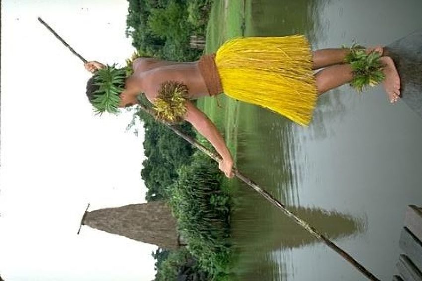

3.1. Directional Total Variation (DTV) tensor at the point i, i.e., (λf)[i] = [λ+ ((S K f)[i]), λ− ((S K f)[i])]T .
 DTV [9] is a local analysis-based regularizer that simply STV also considers a more general case by using φ = k · kq
changes the TV’s rotation invariant ∇ in
 # Eq. (2) with Γ =# (q > 1). Since this design of STV is nonlinear and Eq. (4)
 cos θ − sin θ α 0
 " "
 involves a convolution kernel, the authors of [14] reformulated
Λα R−θ ∇, where Rθ = and Λα =
 sin θ cos θ 0 1 (S K f)[i] in terms of another operator that they named as patch-
with θ ∈ [0, π) corresponding to the dominant direction based Jacobian JK : RN×C 7→ RN×LC×2 , which embodies the
(cos θ, sin θ), and α that is used to tune the dose of the penaliz- convolution kernel of size L, and enables to express the STV
ation. In this way, it penalizes the magnitudes of the scaled and functional such that it can be decomposed into linear function-
rotated gradients, towards a predetermined direction. As men- als. (JK f)[i] is defined as:
tioned earlier, DTV can only be applied to the uni-directional
images. EADTV [10] is its adaptive extension that suggests to (JK f)[i] = (∇f
  ˜ 1 ˜ C )[i]T
 ˜ 2 )[i] · · · (∇f
 )[i], (∇f (6)
use spatially varying angles θ[i]. Even it is trivial to estimate
 where (∇f ˜ c )[i] = (T1 ∇fc )[i], (T2 ∇fc )[i], · · · , (TL ∇fc )[i]. Each
 
a scalar θ from an observed uni-directional image, when θ rep-
resents an orientation field, it becomes a challenging problem. l-th entity applies
 p shifting and weighting on the gradient as
EADTV simply computes each θ[i] such that, (Tl ∇fc )[i] = Kσ [pl ](∇fc )[xi − pl ], where xi denotes the ac-
 tual 2D coordinates of the i-th pixel, and for L = (2LK + 1)2 ,
 (cos θ[i], sin θ[i]) ⊥ (∇gσ )[i] (3) pl ∈ {−LK , · · · , LK }2 is the shift amount. That way, the structure
 tensor in terms of the patch-based Jacobian is:
where the subscript σ indicates that the image g is pre-
smoothed by a Gaussian filter of standard deviation σ. How- (S K f)[i] = (JK f)[i](JK )f)[i]T (7)
ever, the gradient is not a convenient descriptor under extens-
ive amount of noise. The estimation of the gradient is mostly Now, the rooted eigenvalues of (S K f)[i] coincide with the singu-
misguided, and since DTV is sensitive along the angles θ[i], lar values of (JK f)[i], and by employing Sq matrix norm, STV
the structure is destroyed by the incorrect estimates. Moreover, is redefined as:
rippled values of the angles cause unstable output. N
 X
 By recalling Eq. (2), the recent paper [11] plugs Γ = S T V(f) = k(JK f)[i]kSq (8)
Λα (g)R−θ(g) ∇, φ = k · k2 , and p ∈ (0, 1) where Λα and θ are i=1
both functions of g. Except the preference of the outer norm,
 This redefinition allows one to find an efficient numerical solu-
this definition differs from the EADTV in the sense that it better
 tion to STV regularized problems, by using convex optimiza-
recognizes the local edge orientations due to the more complex
 tion tools.
OFE method that it employs, and uses an adaptive stretching
matrix weighted according to the first-order local edge inform-
ation. 4. Proposed Method

3.2. Structure Tensor Total Variation (STV) Let us first point out the relation between the DTV and STV
 measures. By expanding the DTV measure, one can draw the
 The structure tensor of an image f at a point i is a 2 × 2
 following conclusion:
symmetric positive semi-definite (PSD) matrix of the form:
 αDθ f
 " #
 (S K f)[i] = Kσ̂ ∗ ((Jf)[i](Jf)[i]T ) (4) DT V(f) , kΛα R−θ ∇fk1,2 = (9)
 Dθ ⊥ f 1,2
where Kσ̂ is a Gaussian kernel of standard deviation σ̂ centered
at the i-th pixel, and J denotes the Jacobian operator that ex- where Dθ denotes the directional derivative of f in the direction
tends the gradient for vector-valued images, i.e., characterized by θ, and θ⊥ = θ ± π/2. Eq. (9) shows that DTV
 actually works by increasing the dose of penalization (with the
 (Jf)[i] = (∇f1 )[i] (∇f2 )[i] · · · (∇fC )[i] weight α) in the direction that it presumes the variation is min-
  
 (5)
 imum. The penalty dose in the direction of maximum variation,
The superscripted f’s are denoting the channels, and for scalar- which is orthogonal to that of the minimum, is only determined
valued images, J(·) = ∇(·). This semi-local descriptor can sum- by the regularization parameter τ. This idea of penalizing the
marize all the gradients within the patch supported by Kσ̂ , thus maximum and minimum directional variations coincides with
provides a better way of characterizing the variations, when the STV. However, instead of making assumptions, STV codi-
compared to the local differential operators. The eigenvectors fies the maximum and the minimum directional variations with
of it correspond to the directions of maximum and minimum the maximum and the minimum eigenvectors √ and√the square
vectorial variations, and the rooted eigenvalues serve as a meas- roots of the corresponding eigenvalues ( λ+ and λ− ) of the
ure of variations towards the respective directions. At this point, structure tensor. In other words, it deduces the directional vari-
the STV prior [14] presents an innovatory way of describing the ation from a summary of all derivatives within a local neighbor-
total amount
 √ of variations. It replaces the TV’s ∇ in Eq. (2) with hood. " √
 λ+ (S f)
 #
Γ = λ(·), where (λf)[i] is a 2D vector composed of the max- √ − K
 S T V(f) , (10)
imum λ+ (·) and the minimum λ− (·) eigenvalues of the structure λ (S K f) 1,q
 3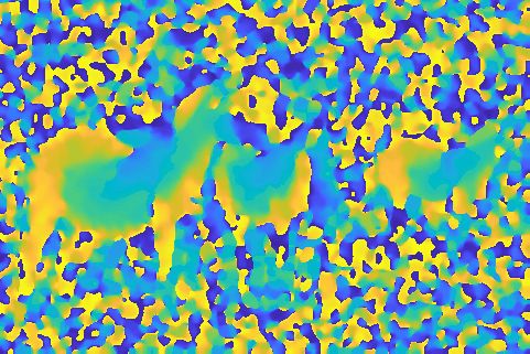

From this point of view, the question that motivated us to design in the regions with isotropic structures, where the correspond-
a direction-guided STV was: Can STV more accurately deduce ing values of α[i] are small. To compensate it, we suggest to use
the directional variation if the summarized derivatives are dir- a scaling matrix Λ̃(α+ ,α- [i]) with two parameters, one of which is
ectional in a pre-determined direction? coming from a spatially varying field of α- : Ω 7→ [1, α+ ]C , i.e.,
 " +
 α
 #
 0
4.1. Direction-Guided STV (DSTV) Λ̃(α+ ,α- [i]) = (13)
 0 α- [i]
 While it has been shown that the STV produces the state-
of-the-art results among the other analysis-based local regular- While at a point i within a highly directional region, α- [i] = 1;
izers; under excessive amount of noise, it may not distinguish in a flat region, it switches to isotropic behavior: α- [i] = α+ .
the edges and may smooth out them. At this point, the DSTV When it comes to the values between these two end points, as
[27] comes into play. It aims at incorporating the prior know- they get closer to one, the sensitivity to the changes towards θ[i]
ledge on the underlying image’s local geometry into STV. Un- increases.
der the inspiration of DTV, DSTV employs directional derivat-
 As a consequence, the directional patch-based Jacobian op-
ives by applying the operator Π(α,θ) that can act on the gradient
at each image point as (Π(α,θ) ∇ f c )[i] = Λα R−θ (∇ f c )[i], while erator given in Eq. (11) is extended to its adaptive version
gathering the neighboring gradients to constitute the patch- (which will be denoted as J˜K(α,θ) ) that employs (Π̃(α,θ) ∇fc )[i] =
based Jacobian as: Λ̃(α+ ,α- [i]) R−θ[i] (∇fc )[i] to perform directional derivation. There-
 fore, our ADSTV regularizer is defined as follows:
(JK(α,θ) f )[i] =
 N
  (T1 Π(α,θ) ∇ f 1 )[i] (T2 Π(α,θ) ∇ f 1 )[i] ··· (TL Π(α,θ) ∇ f 1 )[i] 
   X
  (T1 Π(α,θ) ∇ f 2 )[i] (T2 Π(α,θ) ∇ f 2 )[i] ··· (TL Π(α,θ) ∇ f )[i] 
 2  ADS T V(f) , k( J˜K(α,θ) f)[i]kSq = k J˜K(α,θ) fk1,q (14)
 .. .. .. .. i=1
  
 . . . .
  
  
 
 (T1 Π(α,θ) ∇ f c )[i] (T2 Π(α,θ) ∇ f c )[i] ··· (TL Π(α,θ) ∇ f )[i]
 c 4.3. Parameter Estimation
 (11) Estimation of the parameters α− and θ is not a trivial task.
 In a noisy image, line-like structures are often interrupted by
JK(α,θ) is named as directional patch-based Jacobian [27], and involved the noise, which results in deviations from the correct direc-
by the DSTV functional, i.e., tion. When the conventional smoothing filters are applied to
 N
 X suppress noise, the same line-like structures get thicker, and the
 DS T V(f) = k(JK(α,θ) f)[i]kSq (12) edges are dislocated. The reconnection of the interrupted lines
 i=1 is concerned in many studies, such as the ones that employ the
 morphological operators for the curvilinear structures in bio-
 By means of Eq. (12), one has the chance of leading the STV
 medical images [28, 29], or for the ridges in fingerprint images
machinery in favor of a predetermined direction. It has been ex-
 [30]. Their principle goal is detection rather than restoration.
perimentally shown on uni-directional images in [27] that this
 In the proposed method, we focus finding a layout for the ori-
incorporation produces prominently better results. Also, since
 entations rather than a precise field of them. By means of that,
the convexity is preserved in DSTV, the same convex optimiz-
 the preprocessor does not put much computational overhead.
ation tools used to solve STV can be applied to DSTV based
 In our preprocessor, we employ eigenvectors and eigenvalues
problems.
 of the structure tensor to extract the knowledge about the ori-
 entations and the dose of anisotropy, in semi-local fashion, in
4.2. Adaptive DSTV (ADSTV) contrast to EADTV. We also employ isotropic TV regulariza-
 In natural images, the dominant directions vary in different tion to circumvent the problem of interrupted lines and to ignore
regions, which makes DSTV inapplicable. In order to handle the insignificant deviations. Below, we explain our parameter
arbitrary natural images, we employ the same way that EADTV estimation procedure, which we will refer to as directional para-
employed when bringing adaptivity to DTV. We consider θ as a meter estimator (DPE), step by step in detail. Note that our pre-
spatially varying field of orientation, i.e., θ : Ω 7→ [0, π)C , and processor employs Sobel operator as the discretization scheme
this changes the rotation matrix to R−θ[i] . used for the gradient. Also note that, our parameter estimator
 Furthermore, in natural images, the anisotropic structures uses the luminance information of the input image (gL ), there-
are not homogeneously distributed. Also among the aniso- fore for the vector-valued images, each channel of the θ will
tropic structures, their degrees of anisotropy spatially change. be a copy of each other, i.e., θ1 = θ2 = · · · = θC ). The same
DSTV’s stretching matrix Λα uses a constant factor α for the applies to α− .
entire image. Just as done to the rotation parameter, one may As a measure of anisotropy, we equip a field of coherence
employ a field of spatially changing stretching factors, so that measures c : Ω 7→ [0, 1] computed at each image point as fol-
the dose of penalization at a point can be tuned. However, since lows:
 λ+ [ j] − λ− [ j]
the regularization parameter τ is a constant scalar, with vary- cσ [ j] = σ + σ (15)
ing stretching factor the total amount of regularization changes λσ [ j]
from region to region. The fittest value of τ for a directional re- where λ±σ [ j] = λ± ((S K gLσ )[ j]) and j = {1, 2, · · · , N}. Note
gion that requires larger values of α[i] may produce poor results that in this section, the variables subscripted by σ denote the
 4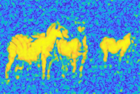

pre-smoothed version of gL not only with the Gaussian ker- α− [ j].
nel of standard deviation σ, but also with the support σ2 × σ2 .
Moreover, the kernel Kσ̄ embodied by the structure tensor that α+ − 1
 α− [ j] = (max(φ) − φ[ j]) + 1 (19)
we employ here operates σ̄ larger than σ̂, again with the sup- max(φ) − min(φ)
port σ̄2 × σ̄2 . Eq. (15) is nothing but a measure of the contrast
 When it comes to the estimation of θ, we first consider the
between the directions of the highest and lowest fluctuations.
 eigendirections of the structure tensor, computed at a scale with
For a pure local orientation (λ+σ > 0, λ−σ = 0) the coherence is
 the highest response to Eq. (17), i.e.,
one, while for an isotropic structure (λ+σ = λ−σ > 0) it is zero.
After computing cσ , by treating it as a corrupted image, we ap- ϑ[ j] = ∠ v−σ̂k [ j], σ̂k = argmax κ̂σk [ j] (20)
ply TV-based regularization. This way, the fluctuating intens- σ1

(a) c(1) (b) φ(1) (c) α− (d) θ

Figure 1: Exemplary outputs of the DPE procedure. The colormaps respectively show (a) the coherence field of unsmoothed gL , (b) its TV regularized version, (c)
the final weights, and (d) the final directions for the noise level ση = 0.15.

 where s = (c − 1)L + l and t = (c − 1)N + n with 1 ≤ n ≤ N and
 1 ≤ c ≤ C. Tl∗ corresponds to the adjoint of Tl , which scans the
 
 X[i, s] in column-wise manner, where X[i, s] ∈ R2 is the s-th
 row of the i-th submatrix of an arbitrary X ∈ RN×LC×2 . Also, the
 operator div is discrete divergence, applied by using backward
 differences, since the gradient is discretized using forward dif-
 ferences, ∗as in [14]. From this point of view, in order to define
 α+
 our J˜K(α,θ) : RN×LC×2 7→ RNC , one should only change the di-
 α-[j] vergence operator in Eq. (25) with the directional divergence
 operator divf (α[i],θ[i]) , i.e.,

 L
 X
 ∗
 Figure 2: A rough illustration of the DPE procedure vs. ADSTV denoiser.
 ( J˜K(α,θ) X)[t] = f (α[i],θ[i]) (T ∗ X[i, s])
 −div l (26)
 l=1

where C is a set corresponding to an additional constraint whose definition is given below:
(C = RNC in unconstrained case). The solution to this f (α[i],θ[i]) (·) , div Π̃T 

 div (α[i],θ[i]) (·)
problem corresponds to the proximal map of ADS T V(f), i.e., (27)
 = div Rθ[i] Λ̃(α+ ,α- [i]) (·)
 

proxτADS T V (g). In [27], proxτDS T V (g) was solved through the
derivation of dual problem in detail. Having ADSTV instead
of DSTV does not change the primal problem, hence the way
that we derive dual will remain same. However, DSTV was
 Let us call the objective function in Eq. (24) as L(f, Ψ).
only considering Frobenius norm (q = 2). We define ADSTV
 It is convex w.r.t. f and concave w.r.t. Ψ. By following the
in more general form, considering q ≥ 1, as a direct extention
 fast gradient projection (FGP) method [32], which combines
of STV. In this respect, to come up with a concise derivation,
 the dual approach introduced in [33] to solve TV-based denois-
using the fact that the dual of the norm k · kSq is k · kS p , where
 ing, and the fast iterative shrinkage-thresholding (FISTA) [34]
q + p = 1, one can redefine ADSTV in terms of the support
1 1
 to accelerate convergence, one can swap min and max, i.e.,
function of the form:
 min max L(f, Ψ) = L(f̂, Ψ̂) = max min L(f, Ψ) (28)
 ADS T V(f) = sup h J˜K(α,θ) f, Ψi (23) f∈C Ψ[i]∈BS p Ψ[i]∈BS p f∈C
 Ψ[i]∈BS p
 since the common saddle point is not affected. Maximization of
by introducing a variable Ψ ∈ RN×LC×2 , and the set BS p = {X ∈ the dual problem d(Ψ) = minf∈C L(f, Ψ) at the right-hand side
RLC×2 : kXkS p ≤ 1}. Here Ψ[i] refers to the i-th submatrix of is same with the minimization of the primal problem P(f) =
Ψ. This paves the way for rewriting the problem in Eq. (22) as maxΨ[i]∈BS p L(f, Ψ) at the left-hand side. Therefore, finding the
a minimax problem: maximizer Ψ̂ of d(Ψ) serves to find the minimizer f̂ of P(Ψ).
 1 ∗
 One can rewrite f̂ in terms of Ψ, as:
 min max kg − fk22 + τhf, J˜K(α,θ) Ψi (24) ∗
 f∈C Ψ[i]∈BS p 2 f̂ = argmin kf − (g − τ J˜K(α,θ) Ψ)k22 − M (29)
 f∈C
 ∗
where J˜K(α,θ) arising after we leave f alone in the second term
denotes the adjoint. The adjoint of the patch-based Jacobian by expanding L(f, Ψ) and collecting the constants under the
JK∗ : RN×LC×2 7→ RNC was defined in [14] with its derivation: term M. The solution to Eq. (29) is:
 ∗
 L
 X f̂ = PC (g − τ J˜K(α,θ) Ψ) (30)
 (JK∗ X)[t] = −div(Tl∗ X[i, s]) (25)
 l=1
 where PC is the orthogonal projection onto the set C. Then we
 6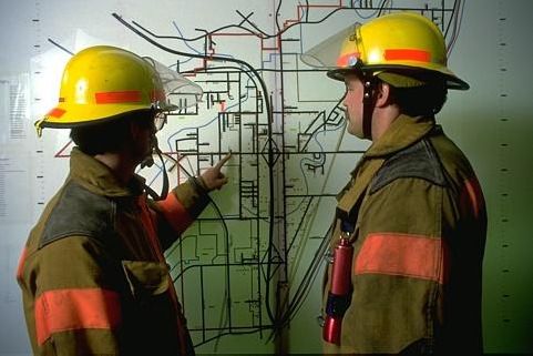

Algorithm 1 Algorithm for ADSTV-based denoising 5. Experiments
 +
 INPUT: g, α > 1, τ > 0, p > 1, PC
 INIT: Ψ(0) = 0 ∈ RN×LC×2 , t(1) = 1, i = 1 In this section, we assess qualitative and quantitative per-
 (θ, α− ) ← DPE(g, α+ ) [Section 4.3] formances of the proposed variational denoising framework.
 √
 L ← 8 2τ (α+ )2 + (α− )◦2 We compare it with the other related analysis-based regular-
 


 while stopping criterion is not satisfied do izers: TV (as a baseline), EADTV (as a representative of previ-
 ∗
 z ← PC (g − τ J˜K(α,θ) Ψ(i−1) ) ous attempts to make DTV [9] adaptive), STV [14] (as a prede-
 

 Ψ(i) ← PBS p Ψ(i−1) + L◦−1 J˜K(α,θ) z cessor of ADSTV), and NCDR [22] (as a recent analysis-based
 (Ψ(i+1) , t(i+1) ) ← FISTA (t(i) , Ψ(i) , Ψ(i−1) ) regularization scheme depending on a new paradigm). We don’t
 i←i+1 include TGV [6] in the competing algorithms since, STV’s su-
 end while periority over it has already been demonstrated in [14]. Ow-
 ∗
 return PC (g(k) − τ J˜K(α,θ) Ψ( j) ) ing to the fact that TV, EADTV, and NCDR are only applic-
 able to the scalar-valued images, they are only involved in the
 function FISTA√(t, f(cur) , f(prev) ) [34] grayscale environment. Thus, the experiments on the vector-
 t(next) ← (1 + 1 + 4t2 ) 2 valued images merely compare STV and DSTV regularizers.
 

 f (next)
 ←f (cur)
 + ( t(next) )(f(cur) − f(prev) )
 t−1 The source codes of STV 2 and NCDR 3 that we use were made
 return (f ,t
 (next) (next)
 ) publicly available by the authors on GitHub. Our ADSTV is
 end implemented on top of STV, while TV and EADTV are written
 from scratch. All methods were written in MATLAB by only
 making use of the CPU. The runtimes were computed on a com-
 puter equipped with Intel Core Processor i7-7500U (2.70-GHz)
 with 16 GB of memory.
 To assess the quantitative performances of the methods, we
proceed by plugging f̂ in L(f, Ψ) to get d(Ψ) = L(f̂, Ψ), i.e., use peak signal-to-noise ratio (PSNR) in dB and structural sim-
 1 1 ilarity index (SSIM). The experiments are performed on the im-
 d(Ψ) = kw − PC (w)k22 + (kgk22 − kwk22 ) (31) ages shown in Figure 3. The first row shows the thumbnails of
 2 2
 seven classical grayscale test images of sizes 256 × 256 (Mon-
 ∗
where w = g − τ J˜K(α,θ) Ψ. Dual problem is smooth with a well- arch, Shells, and Feather) and 512 × 512 (the others). In the
defined gradient computed: other two rows, we have RGB color images. Plant, Spiral, Rope
 ∗
 and Corns of sizes 256 × 256 are more textural with different
 ∇d(Ψ) = τ J˜K(α,θ) PC (g − τ J˜K(α,θ) Ψ) (32) directional characteristics. Rope and Corns are taken from the
 popular Berkeley Segmentation Dataset (BSD) [31], while the
based on the derivation in Lemma 4.1 of [32]. Therefore, in others are public domain images. The rest of the color images
order to find the maximizer Ψ̂ of d(Ψ), one can employ the are natural images taken from BSD. They have either no or lim-
projected gradients [33]. It performs decoupled sequences of ited amount of directional parts. Note that, the intensities of all
gradient descent/ascent and projection onto a set. For the gradi- test images have been normalized to the range [0, 1].
ent ascent in our case, an appropriate step size that ensures the The algorithms under consideration are all aiming to minim-
convergence needs to be selected. For the gradient in Eq. (32), ize Eq. (1). Therefore, the critical regularization parameter τ
a LC × 2 matrix filled by a constant step size 1/L[i] can be used is in common, and should be chosen precisely. For a fair com-
for each image point, where L ∈ RN×LC×2 is a multidimensional parison, we fine-tuned τ such that it leads to the best PSNR
array of Lipschitz
 √ constants each of 
which having the upper in all experiments. For STV, ADSTV, and NCDR priors; one
bound L[i] ≤ 8 2τ2 (α+ )2 + (α− [i])2 . One can see Appendix should also choose the convolution kernel. We used a Gaussian
A for the derivation. kernel of support 3 × 3 for all three algorithms. The standard
 deviations (σ) were set to 0.5 for STV and DSTV, while σ = 1
 When it comes to the projection, as an efficient way, the was used for NCDR, as suggested in the algorithms’ respective
authors of [14] reduced the projection of each Ψ[i] onto BS p papers: [14] and [22]. Both STV and ADSTV use the nuclear
to the projection of the singular values onto the ` p unit ball norm of the patch-based Jacobian, since it was chosen as the
B p = {σ ∈ R2+ : kσk p ≤ 1}. Therefore, for the SVD best performing norm. Similar to the convolution kernel, all the
Ψ[i] = UΣVT and Σ = diag(σ), where σ = [σ1 , σ2 ], the pro- other parameters of NCDR were kept same as they were used
jection was defined as: in [22]. The EADTV’s α is fine-tuned by changing it from 2
 (since it reduces to TV when α = 1) to 30 with 1-unit inter-
 PBS p (Ψ[i]) = Ψ[i]VΣ+ Σp VT (33) vals. This is also the case for the ADSTV’s α+ , unless other-
 wise stated. DSTV requires an additional convolution kernel
where Σ+ is pseudoinverse of Σ and Σ p = diag(σ p ) for σ p are
the projected singular values of Σ. The readers are referred to
[14] for the details about the derivation and the realization. As 2 https://github.com/cig-skoltech/Structure Tensor Total Variation
a consequence, the overall algorithm is shown in Algorithm 1. 3 https://github.com/HUST-Tan/NCDR

 7

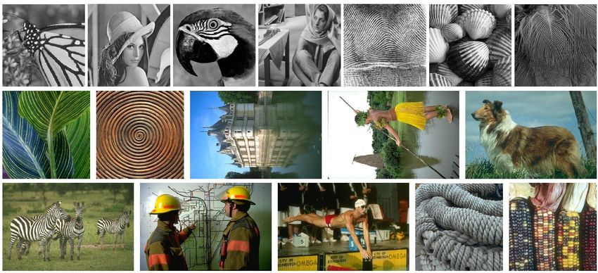
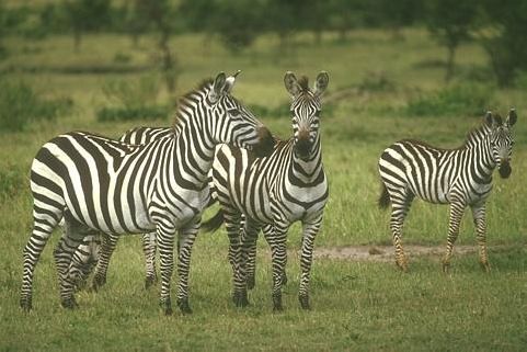
Figure 3: Thumbnails of the grayscale and color images used in the experiments. From left to right and top to bottom: Monarch, Lena, Parrot, Barbara, Fingerprint,
Shells, Feather, Plant, Spiral, Chateau, Indigenous, Dog, Zebra, Workers, Swimmer, Rope, and Corns.

too, to be used by the preprocessor DPE. We fixed it as a Gaus- and Shell. However, as one may see in the last column, these
sian kernel with variance and support σ̄2 = 7 for 256 × 256 results are obtained at the cost of computational load. The av-
images, while σ̄2 = 11 for 963 × 481 natural images from BSD, erage runtimes of NCDR at all noise levels are pretty high. On
and σ̄2 = 15 for 512 × 512 images. For the optimization of all the other hand, when the quality is measured by SSIM, our AD-
TV-based algorithms, the stopping criterion was either having STV systematically outperformed NCDR (and the others). Fig-
a relative normed difference between two successive estimates ure 4 is provided for the visual judgement. It can be inferred
that reaches a threshold of 10−5 , or fulfilling a number of iter- that NCDR smooths the structural regions better than ADSTV
ations, equals to 100 in our case. When it comes to NCDR, at the risk of loss of details (See (d)-(e), (i)-(j), and the scarf
since it uses gradient descent to solve its non-convex optimiza- of Barbara in (s)-(t)). NCDR also causes artifacts in the junc-
tion problem, it is quite hard to ensure that whether a reported tions more apperant than those of ADSTV (e.g., (d)-(e)). Also
result is due to a local or a global minimum. The number of the ADSTV is better at smoothing flat region as one can see on
iterations for NCDR was experimentally set to 500. Lena’s face in (n)-(o). These may clarify why the SSIM values
 We consider additive i.i.d. Gaussian noise with five noise obtained by ADSTV are higher.
levels of ση = { 0.05, 0.1, 0.15, 0.2, 0.25}. In Table 1, we re- Table 2 on the other side, shows PSNR/SSIM values obtained
port PSNR and SSIM measures obtained by using TV, EADTV, by the application of STV and ADSTV to vector-valued images.
STV, NCDR, and ADSTV priors applied to the grayscale im- According to the results, ADSTV systematically outperformed
ages. From the results, we observe that the EADTV does not STV in terms of PSNR and SSIM measures, even in the images
offer significant improvements over TV in the images with less that do not exhibit directional dominance. However, in terms
directional patches such as Lena and Parrot. But, it even per- of the runtimes that are reported in the last row, ADSTV seems
forms worse than TV for Barbara and Feather images, in which to bring almost twice as much load to the computation. Again
highly directional parts present, as the noise level increases. in Figure 5, we demonstrate exemplary detail patches cropped
This is due to the fact that, those directional parts involve very from the original images (first column), noisy versions (second
high frequency components. Thus, even small deviations in the column), and the restored versions by STV (third column) and
direction estimation extremely affects the result. In almost all ADSTV (last column). The results obtained by STV have oil-
of the experiments, EADTV preferred to use α = 2 (except painting-like artifacts, whereas this effect is far less visible in
Fingerprint for which larger α values are selected), and this is ADSTV’s results. With the incorporation of the directional
also due to the need of compensating the sheer amount of mis- information, the edges became more apparent, (see Rope and
takes made by its direction estimator. STV produced signific- Chateau), more smoothing towards the desired direction (see
antly better results when compared to TV and EADTV for all Spiral), and the gaps between closely parallel lines could better
cases and images, except Fingerprint, where for all the noise be distinguished (e.g. the feather in Dog image, the details of
levels ση > 0.1, EADTV outperformed STV. When it comes the leaves in Corns image, and skirt in Indigenous image).
to NCDR, it yielded superior PSNR results to all competing al- One of the ADSTV’s disadvantages is introducing an ex-
gorithms including ADSTV, except the experiments on Parrot tra free parameter α+ that needs to be tuned. In Figure 6, we
 8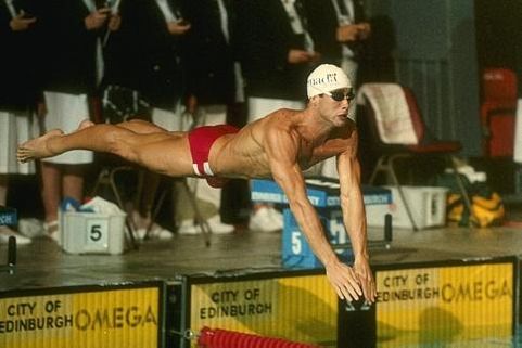

Table 1: PSNR/SSIM Comparison of TV, EADTV, STV, NCDR, and ADSTV on grayscale images. Last column shows the average runtimes.

 Monarch Lena Parrot Barbara Fingerp. Shell Feather Avg. t (sec.)
 TV 31.54/0.91 32.88/0.87 33.17/0.88 29.48/0.84 29.14/0.93 28.69/0.89 26.79/0.93 30.24/0.89 1.51
ση = 0.05

 EADTV 31.91/0.92 33.09/0.87 33.16/0.88 29.59/0.83 29.73/0.94 28.81/0.89 26.86/0.93 30.45/0.89 1.82
 STV 32.32/0.93 33.59/0.88 33.56/0.90 30.19/0.88 30.11/0.94 29.01/0.89 27.16/0.94 30.85/0.91 17.41
 NCDR 32.66/0.93 34.26/0.89 33.40/0.90 31.44/0.89 30.08/0.94 29.24/0.89 28.47/0.94 31.36/0.91 276.98
 ADSTV 32.61/0.93 34.03/0.89 33.77/0.91 31.09/0.89 30.09/0.94 29.36/0.90 27.89/0.95 31.25/0.92 38.24
 TV 27.88/0.85 29.86/0.81 29.74/0.82 25.57/0.71 25.33/0.86 24.94/0.77 21.95/0.81 26.47/0.80 2.08
 EADTV 28.31/0.84 30.07/0.81 29.81/0.81 25.51/0.70 25.83/0.87 24.45/0.76 21.65/0.81 26.52/0.80 2.77
ση = 0.1

 STV 28.65/0.87 30.54/0.83 30.22/0.84 26.45/0.77 26.21/0.87 25.34/0.79 22.40/0.83 27.12/0.83 16.92
 NCDR 29.29/0.88 31.36/0.84 30.31/0.85 27.56/0.80 26.54/0.88 25.74/0.79 24.32/0.84 27.88/0.84 256.77
 ADSTV 29.07/0.88 31.15/0.84 30.47/0.85 27.34/0.81 26.48/0.88 25.83/0.81 23.60/0.86 27.70/0.85 34.59
 TV 25.84/0.80 28.23/0.77 27.91/0.77 23.88/0.64 23.30/0.79 23.06/0.68 19.58/0.67 24.54/0.73 2.28
ση = 0.15

 EADTV 26.24/0.80 28.38/0.77 28.02/0.77 23.78/0.63 24.22/0.82 23.22/0.69 19.03/0.67 24.70/0.74 3.07
 STV 26.58/0.82 28.85/0.79 28.43/0.79 24.47/0.69 24.20/0.81 23.48/0.71 20.04/0.70 25.15/0.76 16.77
 NCDR 27.34/0.84 29.61/0.80 28.69/0.80 25.47/0.72 24.64/0.82 24.00/0.70 22.00/0.72 25.96/0.77 270.70
 ADSTV 27.02/0.84 29.45/0.81 28.73/0.81 25.40/0.74 24.46/0.81 24.04/0.73 21.30/0.76 25.76/0.79 31.63
 TV 24.43/0.75 27.14/0.74 26.68/0.73 23.04/0.61 21.94/0.72 21.87/0.61 18.21/0.54 23.33/0.67 2.78
 EADTV 24.78/0.76 27.22/0.74 26.77/0.73 22.96/0.60 22.80/0.77 22.00/0.62 18.12/0.54 23.50/0.68 2.58
ση = 0.2

 STV 25.13/0.78 27.69/0.76 27.22/0.76 23.45/0.65 22.68/0.76 22.27/0.64 18.65/0.58 23.87/0.70 16.21
 NCDR 25.92/0.80 28.35/0.78 27.56/0.77 24.21/0.66 23.28/0.77 22.81/0.63 20.35/0.60 24.64/0.72 269.34
 ADSTV 25.61/0.80 28.29/0.78 27.59/0.78 23.98/0.67 23.12/0.77 22.79/0.66 19.66/0.65 24.43/0.73 36.77
 TV 23.35/0.72 26.33/0.71 25.75/0.71 22.52/0.58 20.93/0.67 21.02/0.55 17.38/0.42 22.47/0.62 2.76
ση = 0.25

 EADTV 23.64/0.72 26.35/0.72 25.82/0.71 22.48/0.58 21.68/0.72 21.13/0.57 17.23/0.41 22.62/0.63 2.82
 STV 24.01/0.75 26.82/0.74 26.30/0.74 22.90/0.61 21.58/0.70 21.40/0.59 17.75/0.47 22.97/0.66 16.60
 NCDR 24.80/0.77 27.37/0.75 26.65/0.75 23.33/0.62 22.16/0.71 21.88/0.57 19.11/0.48 23.61/0.66 274.48
 ADSTV 24.53/0.77 27.37/0.76 26.78/0.76 23.22/0.63 22.11/0.71 21.90/0.61 18.54/0.54 23.49/0.68 36.70

 Table 2: PSNR/SSIM Comparison of STV and ADSTV on color image denoising. Last row shows the average runtimes.

 ση = 0.05 ση = 0.1 ση = 0.15 ση = 0.2 ση = 0.25
 STV ADSTV STV ADSTV STV ADSTV STV ADSTV STV ADSTV
 Plant 29.23/0.96 30.32/0.97 25.27/0.90 26.63/0.93 23.28/0.85 24.60/0.89 22.05/0.80 23.24/0.85 21.21/0.76 22.27/0.81
 Spiral 27.82/0.97 28.39/0.98 24.02/0.93 24.76/0.94 22.04/0.89 23.06/0.91 20.73/0.86 21.95/0.89 19.74/0.83 21.08/0.87
 Chateau 32.43/0.95 32.74/0.96 28.83/0.91 29.39/0.92 26.93/0.87 27.63/0.89 25.75/0.85 26.46/0.87 24.88/0.83 25.51/0.85
 Indigenous 32.70/0.95 33.04/0.96 29.33/0.90 29.74/0.92 27.71/0.88 28.07/0.89 26.70/0.85 26.99/0.87 25.99/0.84 26.25/0.85
 Dog 32.19/0.95 32.53/0.96 29.00/0.90 29.40/0.91 27.44/0.87 27.80/0.88 26.46/0.84 26.76/0.85 25.78/0.82 26.05/0.83
 Zebra 30.70/0.97 30.87/0.97 26.86/0.93 27.46/0.94 24.84/0.90 25.58/0.91 23.46/0.86 24.26/0.89 22.47/0.84 23.34/0.87
 Workers 31.92/0.95 32.41/0.96 28.06/0.90 28.77/0.92 25.96/0.85 26.77/0.89 24.57/0.81 25.39/0.85 23.56/0.77 24.37/0.82
 Swimmer 33.63/0.97 33.92/0.98 30.17/0.95 30.57/0.95 28.29/0.92 28.73/0.93 27.03/0.90 27.43/0.92 26.09/0.88 26.50/0.90
 Rope 28.37/0.91 28.53/0.91 24.68/0.80 24.96/0.81 22.87/0.70 23.18/0.72 21.73/0.61 22.06/0.63 20.93/0.55 21.23/0.58
 Corns 29.74/0.95 29.90/0.95 25.94/0.89 26.16/0.90 23.92/0.83 24.06/0.84 22.59/0.78 22.74/0.79 21.63/0.74 21.77/0.74
 Avg. 30.87/0.95 31.27/0.96 27.22/0.90 27.78/0.91 25.33/0.86 25.95/0.88 24.11/0.82 24.73/0.84 23.23/0.79 23.84/0.81
 t (sec.) 20.62 40.18 21.32 33.81 18.97 33.39 21.12 36.27 22.50 35.54

present two graphs to show how sensitive the gain over STV by 6. Discussion
using our method with respect to α+ is. Figure 6 (a) serves the
purpose by testing varying α+ values on five different grayscale In the previous section, we compared the proposed denoising
and color images at the noise level ση = 0.15, while Figure framework with TV [1], EADTV [9, 10], STV [14], and NCDR
6 (b) examines them on Barbara image at five different noise [22] based denoising models. STV was holding the state-of-the-
levels. As one can infer from the results, even for the incorrect art records among the other TV-related local analysis-based pri-
selections of α+ , the gain has almost always been above zero, ors. NCDR came up with a new paradigm regarding the sparsity
which shows the robustness of our approach. Yet a relevant of the corner points, in 2018. Although the NCDR puts plaus-
research question here might be if it is possible to calculate α+ ible results out, its non-convexity and heuristic nature make it
automatically, as a function of an estimated noise level by using disadvantageous. Moreover, it’s only applicable to the scalar-
variance estimators and coherence. valued images. The qualitative results and SSIM measurements
 show the effectiveness of our ADSTV over NCDR in terms of
 9

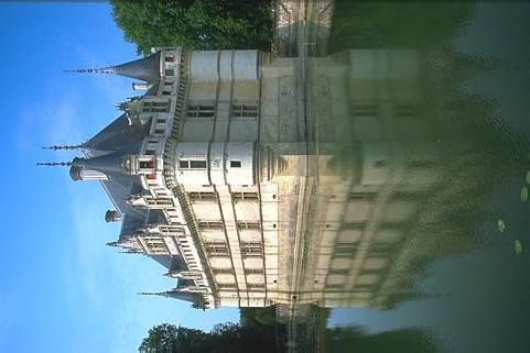
Figure 4: The detail patches showing grayscale image denoising results. The noisy Barbara (ση = 0.1), Feather, Lena (ση = 0.15), and Fingerprint (ση = 0.2)
images are restored by using TV (col-1), EADTV (col-2), STV (col-3), NCDR (col-4), and ADSTV (col-5) regularizers. The quantity pairs shown at the bottom of
each image are corresponding to the (PSNR, SSIM) values.

restoration quality, while NCDR results in better PSNR. But We think this difference is due to the incorporation of structure
when we consider the computational performances, NCDR ma- tensor.
chinery is around 7 times slower than ADSTV. We believe that Finally, in order not to finish discussion without referring to
our framework provides a good balance between the restoration today’s learning based approaches on restoration, we want to
quality and the computational performance. touch upon briefly how close our results to those obtained by
 On the other hand, as mentioned in Sect. 1 and Sect. 3.1, the popular feed-forward denoising convolutional neural net-
a closely related paper [11] was published as prepress (to be works (DnCNN) [35]. On the same Parrot, Lena, and Barbara
published in 2020) at the moment that we were studying on this images of the range [0, 255], the authors of DnCNN experi-
paper. That work couldn’t be involved in our experiments but, mented three noise levels {15, 25, 50} and reported the PSNR
due to the common experiment performed on the same Lena scores. When we perform the same experiments on the Par-
image, we think it is worth talking over it here. The authors re- rot image, we observed that the results of ADSTV were almost
ported that the restored versions of Lena contaminated by Gaus- 1 dB better than DnCNN. However on Lena and Barbara im-
sian noise with σ = {0.05, 0.1, 0.15} has the signal to noise ra- ages it was not the case, and DnCNN performed around 1 dB
tio (SNR) around 17.5, 15 and, 13, respectively; whereas the and 1.5 dB better than ADSTV, respectively, as might be ex-
corresponding results of ADSTV are 19.77, 16.84, and 15.07. pected. Similar to the classification tasks, data-driven meth-
 10

Figure 5: The detail patches showing color image denoising results. The noisy Indigenous, Dog (ση = 0.15), and Rope, Spiral, Corns, Chateau, Indigenous (ση =
0.2) images (col-2) are restored by using STV (col-3) and ADSTV (col-4) regularizers. The quantity pairs shown at the bottom of each image are corresponding to
the (PSNR, SSIM) values.

ods seems to predominate the model-driven ones in restoration be used for training purpose, difficulty of incorporating prior
tasks. They can themselves capture the underlying geometry domain knowledge, and the strong dependency to the imaging
within the data. Moreover, they can run very fast once trained. parameters (e.g. noise level) of the training data. To tackle
However, beside those advantages, they also have limitations with these limitations, new efforts try to involve the variational
such as the lack of the suitable ground truth images that would models in the learning-based methods [22, 36, 37]. Also as

 11

1.4 1.2
 Lena = 0.05
 Parrot
 1.2 1 = 0.1
 Feather
 Workers = 0.15
 Swimmer = 0.2
 1 0.8
 = 0.25
 PSNR Gain

 PSNR Gain
 0.8 0.6

 0.6 0.4

 0.4 0.2

 0.2 0

 0 -0.2
 0 5 10 15 20 25 30 0 2 4 6 8 10 12 14 16 18 20
 + +

 (a) ση = 0.15 (b) Barbara

 Figure 6: PSNR gain over STV with respect to α+ .

remarked in [38], the learning-based approaches comprise the a source for the parameters). We plan to pursue this issue as
variational approaches as special cases. These facts and the future work.
non-negligible drawbacks motivate the researchers to produce
in both fields with the hope that their achievements might fur-
 Appendix A
ther be combined.
 In order to find an upper bound for Lipschitz constants, we
 follow the derivation in [32] and adapt it to our formulation.
7. Conclusion
 ∗ ∗
 k∇d(u) − ∇d(v)k = τk J˜K(α,θ) PC (g − τ J˜K(α,θ) u) − J˜K(α,θ) PC (g − τ J˜K(α,θ) v))k
 In this study, we’ve described a two-stage variational frame- ∗ ∗
 ≤ τk J˜K(α,θ) kkPC (g − τ J˜K(α,θ) u) − PC (g − τ J˜K(α,θ) v))k
work for denoising scalar- and vector-valued images. First ∗
stage is the preprocessor that estimates some directional para- ≤ τk J˜K(α,θ) kkτ J˜K(α,θ) (u − v)k
meters that will guide to the second stage, and the second stage ≤ τ2 kΠ̃(α,θ) k2 kJK k2 ku − vk
is the one that performs denoising. Our preprocessor attempts ≤ τ2 kΠ̃(α,θ) k2 k∇k2 kT k2 ku − vk
to circumvent the chicken-and-egg problem of capturing local (34)
geometry from a noisy image to be used while denoise it, by
 where T = l=1
 PL
employing the eigenvalues and the orthogonal eigenvectors of (Tl∗ Tl ). Knowing from [32] that k∇k2 ≤ 8,
the structure tensor, and making assumptions on the piecewise- √
 from [14] that kT k2 ≤ 2, and further showing that kΠ̃(α,θ) k2 ≤
constancy of the underlying directional parameters. When it (α+ )2 + (α− )◦2 , we √
 come up with the spatially varying Lipschitz
comes to the denoising stage, it encodes the problem as a con- constants L[i] ≤ 8 2τ2 ((α+ )2 + (α− [i])2 ).
vex optimization problem that involves the proposed adaptive
direction-guided structure tensor total variation (ADSTV) as
regularizer. Our ADSTV is designed by extending the structure Acknowledgements
tensor total variation (STV), so that it works biased in a cer-
 The authors would like to thank the anonymous reviewers for
tain direction varying at each point in the image domain. This
 their valuable comments and suggestions. This work was sup-
approach results in improved restoration quality that has been
 ported by The Scientific and Technological Research Council
verified by extensive experiments. We compared our method
 of Turkey (TUBITAK) under 115R285.
with the related denoising models involving various analysis-
based priors.
 We believe that the ADSTV regularizer can be used in a large References
spectrum of inverse imaging problems, even though the effect-
 [1] L. I. Rudin, S. Osher, E. Fatemi, Nonlinear total variation based noise
iveness of our preprocessor may change from problem to prob- removal algorithms, Physica D: nonlinear phenomena 60 (1992) 259–
lem. Furthermore, there might be appropriate application fields 268.
where the source image that is used to estimate the directional [2] T. Chan, A. Marquina, P. Mulet, High-order total variation-based image
 restoration, SIAM Journal on Scientific Computing 22 (2000) 503–516.
parameters differs from the target image to be restored (e.g., [3] S. Esedoglu, S. J. Osher, Decomposition of images by the anisotropic
video restoration where the source and target frames are differ- rudin-osher-fatemi model, Communications on pure and applied math-
ent, pansharpening where the chromatic image can be used as ematics 57 (2004) 1609–1626.

 12

[4] R. Chartrand, Exact reconstruction of sparse signals via nonconvex min- logical tools for reconnecting broken ridges in fingerprint images, Pattern
 imization, IEEE Signal Processing Letters 14 (2007) 707–710. Recognition 41 (2008) 367–377.
 [5] Y. Lou, T. Zeng, S. Osher, J. Xin, A weighted difference of anisotropic [31] P. Arbelaez, M. Maire, C. Fowlkes, J. Malik, Contour detection and hier-
 and isotropic total variation model for image processing, SIAM Journal archical image segmentation, IEEE Trans. Pattern Anal. Mach. Intell.
 on Imaging Sciences 8 (2015) 1798–1823. 33 (2011) 898–916. URL: http://dx.doi.org/10.1109/TPAMI.2010.161.
 [6] K. Bredies, K. Kunisch, T. Pock, Total generalized variation, SIAM doi:10.1109/TPAMI.2010.161.
 Journal on Imaging Sciences 3 (2010) 492–526. [32] A. Beck, M. Teboulle, Fast gradient-based algorithms for constrained
 [7] S. Lefkimmiatis, J. P. Ward, M. Unser, Hessian schatten-norm regulariz- total variation image denoising and deblurring problems, IEEE Transac-
 ation for linear inverse problems, IEEE transactions on image processing tions on Image Processing 18 (2009) 2419–2434.
 22 (2013) 1873–1888. [33] A. Chambolle, An algorithm for total variation minimization and applic-
 [8] K. Papafitsoros, C.-B. Schönlieb, A combined first and second order vari- ations, Journal of Mathematical imaging and vision 20 (2004) 89–97.
 ational approach for image reconstruction, Journal of mathematical ima- [34] A. Beck, M. Teboulle, A fast iterative shrinkage-thresholding algorithm
 ging and vision 48 (2014) 308–338. for linear inverse problems, SIAM journal on imaging sciences 2 (2009)
 [9] I. Bayram, M. E. Kamasak, Directional total variation, IEEE Signal 183–202.
 Processing Letters 19 (2012) 781–784. [35] K. Zhang, W. Zuo, Y. Chen, D. Meng, L. Zhang, Beyond a gaussian de-
[10] H. Zhang, Y. Wang, Edge adaptive directional total variation, The Journal noiser: Residual learning of deep cnn for image denoising, IEEE Trans-
 of Engineering 2013 (2013) 61–62. actions on Image Processing 26 (2017) 3142–3155.
[11] Z.-F. Pang, H.-L. Zhang, S. Luo, T. Zeng, Image denoising based on [36] S. Lefkimmiatis, Universal denoising networks: A novel cnn architec-
 the adaptive weighted tvp regularization, Signal Processing 167 (2020) ture for image denoising, in: Proceedings of the IEEE Conference on
 107325. Computer Vision and Pattern Recognition, 2018, pp. 3204–3213.
[12] L. Hong, Y. Wan, A. Jain, Fingerprint image enhancement: algorithm [37] D. Ulyanov, A. Vedaldi, V. Lempitsky, Deep image prior, in: Proceedings
 and performance evaluation, IEEE transactions on pattern analysis and of the IEEE Conference on Computer Vision and Pattern Recognition,
 machine intelligence 20 (1998) 777–789. 2018, pp. 9446–9454.
[13] M. Grasmair, F. Lenzen, Anisotropic total variation filtering, Applied [38] M. T. McCann, K. H. Jin, M. Unser, Convolutional neural networks for in-
 Mathematics & Optimization 62 (2010) 323–339. verse problems in imaging: A review, IEEE Signal Processing Magazine
[14] S. Lefkimmiatis, A. Roussos, P. Maragos, M. Unser, Structure tensor total 34 (2017) 85–95.
 variation, SIAM Journal on Imaging Sciences 8 (2015) 1090–1122.
[15] P. Blomgren, T. F. Chan, Color tv: total variation methods for restoration
 of vector-valued images, IEEE transactions on image processing 7 (1998)
 304–309.
[16] A. Buades, B. Coll, J.-M. Morel, Non-local means denoising, Image
 Processing On Line 1 (2011) 208–212.
[17] G. Gilboa, S. Osher, Nonlocal operators with applications to image pro-
 cessing, Multiscale Modeling & Simulation 7 (2008) 1005–1028.
[18] S. Lefkimmiatis, S. Osher, Nonlocal structure tensor functionals for
 image regularization, IEEE Transactions on Computational Imaging 1
 (2015) 16–29.
[19] A. Chambolle, R. A. De Vore, N.-Y. Lee, B. J. Lucier, Nonlinear wavelet
 image processing: variational problems, compression, and noise removal
 through wavelet shrinkage, IEEE Transactions on Image Processing 7
 (1998) 319–335.
[20] M. A. Figueiredo, J. M. Bioucas-Dias, R. D. Nowak, Majorization–
 minimization algorithms for wavelet-based image restoration, IEEE
 Transactions on Image processing 16 (2007) 2980–2991.
[21] G. Kutyniok, M. Shahram, X. Zhuang, Shearlab: A rational design of a
 digital parabolic scaling algorithm, SIAM Journal on Imaging Sciences 5
 (2012) 1291–1332.
[22] H. Liu, S. Tan, Image regularizations based on the sparsity of corner
 points, IEEE Transactions on Image Processing 28 (2018) 72–87.
[23] G. Gilboa, N. Sochen, Y. Y. Zeevi, Variational denoising of partly textured
 images by spatially varying constraints, IEEE Transactions on Image
 Processing 15 (2006) 2281–2289.
[24] M. Grasmair, Locally adaptive total variation regularization, in: Interna-
 tional Conference on Scale Space and Variational Methods in Computer
 Vision, Springer, 2009, pp. 331–342.
[25] Y. Dong, M. Hintermüller, Multi-scale total variation with automated reg-
 ularization parameter selection for color image restoration, in: Interna-
 tional Conference on Scale Space and Variational Methods in Computer
 Vision, Springer, 2009, pp. 271–281.
[26] R. Bhatia, Matrix analysis, volume 169, Springer Science & Business
 Media, 2013.
[27] E. Demircan-Tureyen, M. E. Kamasak, On the direction guidance in
 structure tensor total variation based denoising, in: Iberian Conference
 on Pattern Recognition and Image Analysis, Springer, 2019, pp. 89–100.
[28] O. Merveille, B. Naegel, H. Talbot, L. Najman, N. Passat, 2d filtering of
 curvilinear structures by ranking the orientation responses of path operat-
 ors (rorpo) (2017).
[29] O. Merveille, H. Talbot, L. Najman, N. Passat, Curvilinear structure ana-
 lysis by ranking the orientation responses of path operators, IEEE trans-
 actions on pattern analysis and machine intelligence 40 (2017) 304–317.
[30] M. A. Oliveira, N. J. Leite, A multiscale directional operator and morpho-

 13