Adaptive Sparse Domain Selection for Weather Radar Superresolution
←
→
Page content transcription
If your browser does not render page correctly, please read the page content below
Hindawi
Scientific Programming
Volume 2022, Article ID 9685831, 12 pages
https://doi.org/10.1155/2022/9685831

Research Article
Adaptive Sparse Domain Selection for Weather
Radar Superresolution

 Haoxuan Yuan ,1,2 Qiangyu Zeng ,1,2 and Jianxin He1,2
 1
 College of Electronic Engineering, Chengdu University of Information Technology, Chengdu 610225, China
 2
 CMA Key Laboratory of Atmospheric Sounding, Chengdu 610225, China

 Correspondence should be addressed to Qiangyu Zeng; zqy@cuit.edu.cn

 Received 26 October 2021; Revised 8 December 2021; Accepted 22 December 2021; Published 11 January 2022

 Academic Editor: Shujaat Hussain Kausar

 Copyright © 2022 Haoxuan Yuan et al. This is an open access article distributed under the Creative Commons Attribution License,
 which permits unrestricted use, distribution, and reproduction in any medium, provided the original work is properly cited.
 Accurate and high-resolution weather radar data reflecting detailed structure information of radar echo plays an important role in
 analysis and forecast of extreme weather. Typically, this is done using interpolation schemes, which only use several neighboring
 data values for computational approximation to get the estimated, resulting the loss of intense echo information. Focus on this
 limitation, a superresolution reconstruction algorithm of weather radar data based on adaptive sparse domain selection (ASDS) is
 proposed in this article. First, the ASDS algorithm gets a compact dictionary by learning the precollected data of model weather
 radar echo patches. Second, the most relevant subdictionaries are adaptively select for each low-resolution echo patches during the
 spare coding. Third, two adaptive regularization terms are introduced to further improve the reconstruction effect of the edge and
 intense echo information of the radar echo. Experimental results show that the ASDS algorithm substantially outperforms
 interpolation methods for ×2 and ×4 reconstruction in terms of both visual quality and quantitative evaluation metrics.

1. Introduction under a high signal-to-noise ratio and equals or exceeds the
 performance of digital matched filter under a low signal-to-
China Next Generation Weather Radar (CINRAD) have noise ratio. Experiments on the WSR-88D (KOUN) radar
been widely applied in operational research and forecast on show that under the same condition, applying adaptive
medium-scale and short-duration strong weather phe- pseudo whitening to the range oversampled signal can re-
nomena. Many of the advantages of the CINRAD are as- duce the standard deviation of the differential reflectivity
sociated with its high temporal (approx. 6 minutes) and estimate to 0.25 dB. Multiscale statistical characteristics of
spatial (approx. 1° × 1 km) resolution. However, the radar reflectivity data in small-scale intense precipitation
problem related to the weak detection capability at long condition are determined.
distances also deserve attention [1, 2]. As shown in Fig- Due to the light computation, interpolation methods are
ure 1, the radar beam width increases with the increase of widely applied in increasing the resolution of radar data to
detection distance, resulting in the accuracy of radar obtain detailed echo structure information. Conventional
products susceptible to beam broadening and ground interpolation methods based on low-pass filtering such as
clutter. bilinear, bicubic, and Cressman interpolation [6, 7] are
 Focusing on IQ data, more high-resolution information featured by easy implementation and high speed of oper-
can be obtained by oversampling the IQ signal in range and ation. However, one of the major limitations is that these
azimuth; next, combine whitening filtering and distance methods mainly use several neighboring data values for
oversampling techniques to obtain better parameter esti- computational approximation to get the estimation and fail
mates [3, 4]. In article [5], authors proposed an operative to exploit the large-scale context information, which leads to
adaptive pseudo whitening technique for single polarization the deficiency in recovering edge and high-frequency in-
radar, which sustains the performance of pure whitening formation of weather radar echo.
2 Scientific Programming

 Storm: Actual 60 dBZ
 core

 “B”
 =6 0 dB
 Z

 “A” < 60 dBZ

 Radar “A” is farther away from the
 storm, so it has a widen beam when
 Radar “B” is closer to the storm,
 detecting the 60 dBZ core
 so it has a narrow beam when
 detecting the 60 dBZ core, which
 Radar “A” completely fills the beam... Radar “B”

 Figure 1: The effect of beam broadening.

 Accurate and fine-grained estimation of high-resolution 2. Literature Review
information benefits from regularization constraints based
on the characteristic of weather radar data. In this article, we This section describes the research work done so far in the
propose an adaptive sparse domain selection (ASDS) al- subject area.
gorithm for superresolution reconstruction of weather radar Torres and Curtis [5] proposed an iterated functions
data, which learn a compact dictionary from a precollected systems (IFS) interpolation method on the basis of bilinear
dataset of example weather radar echo patches by using the interpolation, which effectively utilize the fractal law of
principal component analysis (PCA) algorithm, then the precipitation to downscale satellite remote sensing precip-
most pertinent subdictionaries are adaptively selected for itation products and improved the resolution of input
each low-resolution echo patches during the sparse coding. variables of hydrological model. Fast Fourier transform is
Besides the sparse regularization, autoregressive (AR) and also applied to temporal interpolation of weather radar data,
nonlocal (NL) adaptive regularization are also incorporated which achieve accurate and efficient performance by win-
based on the local and nonlocal spatial characteristic of dowing the input data [8]. The research article [9] proposed a
weather radar data. spline interpolation method to generate satellite precipita-
 Key contributions of the proposed research are as tion estimates with more refined resolution, which slightly
follows: outperformed the methods based on linear regression and
 artificial neural network. The research article [10] proposed
 (1) An efficient superresolution reconstruction algo- an interpolation method to improve the resolution of radar
 rithm of weather radar data based on adaptive sparse reflectivity data, which effectively uses the hidden Markov
 domain selection (ASDS) is proposed in this article tree (HMT) model as a priori information to well capture the
 (2) Two adaptive regularization terms are introduced to multiscale statistical characteristics of radar reflectivity data
 improve the reconstruction effect of the edge and in small-scale strong precipitation condition.
 intense echo information of the radar echo The regularization-based downscaling methods trans-
 form the downscaling problem into a constrained optimi-
 (3) The proposed ASDS algorithm substantially out-
 zation problem by setting up a priori model of the radar echo
 performs interpolation methods for ×2 and ×4 re-
 data. Based on the non-Gaussian distribution of precipita-
 construction in terms of both visual quality and
 tion reflectivity data [11, 12], recast downscaling problem
 quantitative evaluation metrics
 into ill-posed inverse problem to generate high-resolution
 The remaining part of the article proceeds as follows. information by adding regularization constraint based on
Section 2 describes the existing work in the subject area, and Gaussian-scale mixtures model. The research article [13] is
Section 3 discusses the methodology, starting from the brief also selected to solve the inverse problem by exploiting the
introduction of the preliminaries of the article. The proposed statistical properties of spatial precipitation data [8]. Based
ASDS algorithm and its details are provided in Section 4. The on the sparsity of precipitation fields in wavelet domain,
implementation details of ASDS are described in Section 5. sparse-regularization method [14] is applied to obtain high-
Several experimental results and discussions are presented to resolution estimation in an optimal sense. Inspired by the
validate the effectiveness of ASDS in Section 6. Section 7 sparsity and rich amount of nonlocal redundancies in
concludes the article. weather radar data, [15] further incorporate the nonlocal
Scientific Programming 3

regularization on the basis of sparse representation, which optimization problem [20, 21]. Equation (1) can be expressed
achieve promising performance in recovering detail echo as
information. The research article [16] proposed a dictionary
based for downscaling short-duration precipitation events. a � arg min ‖y − DΦa‖22 + λ · ‖a‖1 . (2)
 a
Similarly, in the research article [17], adaptive regularized
sparse representation for weather radar echo super- In equation (2), the l1 norm is the local sparsity con-
resolution reconstruction is discussed. straint to ensure that the sparse coding vector x is sufficiently
 sparse. A number of algorithms, such as iterative threshold
3. Methodology algorithm [22] and Bregman splitting algorithm [23, 24],
 have been proposed to solve equation (2); the reconstructed
This section describes the research methodology proposed high-resolution echo x � Φ a.
for the subject title. In addition,
 √� it√is� assumed that xi is a radar echo patch
 with size of n × n extracted from high-resolution echo x,
3.1. Weather Radar Data: Sparse Representation. In this i.e., xi � Ri x, where Ri represents the window function
section, we present the characteristic of weather radar data extracted from the upper left to the lower right patch with
and give a brief introduction to the sparse representation overlap for x. Using over complete dictionary
related to this article. Φki ∈ Rn×M , n ≪ M the sparse coding vector is obtained by
 minimizing the following equation:
3.2. Characteristic of Weather Radar Data. The level-II data �� ��2 �� ��
 a i � arg min ���yi − DΦki ai ��� + λ · ��ai ��1 . (3)
products used in this article come from S-band China Next ai
 2
Generation Weather Radar (CINRAD-SA). For reflectivity
data, each elevation cut has 360 radials and each radial has Each weather radar echo patch can be sparsely expressed
460 range bins. For radial velocity data, each elevation cut as follows: x i � Φki a i so a series of sparse coding vectors a i
has 360 radials and each radial has 920 range bins. The range and reconstructed high-resolution radar echo patches x i can
resolution of reflectivity and radial velocity data are 1 km be obtained. By averaging all the reconstructed radar echo
and 0.25 km, respectively. The weather radar data include a patches, the whole reconstructed high-resolution radar echo
large number of missing-data values that exceed the coding can be obtained by
threshold or the corresponding range bin is in a region of the
 −1
atmosphere where weather phenomena do not exist N N
[15, 18, 19]. The missing-data statistics of the first elevation x ≈ Φ ∘ a i � ⎡⎣ RTi Ri ⎤⎦ ⎣⎡ RTi x i ⎤⎦, (4)
cut under large- and small-scale weather system and i�1 i�1

cloudless condition is shown in Figure 2, from which we can where N is the number of radar echo patches and equation
see that missing-data has a high percentage of weather radar (2) can be formulated as follows:
data, especially in cloudless condition. Due to the presence
of large amounts of invalid data, weather radar data are a � arg min ‖y − DΦ ∘ a‖22 + λ · ‖a‖1 . (5)
 a
typically featured by high sparsity. Inspired by the sparsity of
weather radar data, it is feasible to apply sparse represen- Rest of the details of the methodology are explained in a
tation for resolution enhancement. separate section 3, discussing the Adaptive Sparse Domain
 Selection Model in its subsequent sections.
3.3. Sparse Representation. The basic idea of sparse repre-
sentation is that a signal x ∈ RN (N is the size of weather 4. Adaptive Sparse Domain Selection Model
radar echo) can be expressed as a linear combination of basis
vectors (dictionary elements); x � Φa and On the basis of sparse representation, the adaptive sparse
Φ ∈ RN×M , N ≪ M are over complete dictionaries, and the domain selection (ASDS) model proposed in this includes
coefficient a satisfies a certain sparse constraint, which can the following: subdictionaries learning and adaptive selec-
be expressed as ‖a‖o ≪ M and ‖•‖0 denotes the l0 norm. tion of the subdictionary and adaptive regularization. An
Using sparse prior, to reconstruct from y to x the sparse adaptive sparse domain selection (ASDS) scheme is a model
coefficient of x in dictionary Φ can be obtained by which learns a series of compact subdictionaries and allo-
 cates adaptively each local patch a subdictionary as the
 a � arg min ‖y − DΦa‖22 + λ · ‖a‖0 , (1) sparse domain.
 a

where parameter λ is the trade-off between sparse repre-
sentation and reconstruction error, and l0 norm is used to 4.1. Subdictionaries Learning. Dictionary learning is a key
calculate the number of nonzero elements in coefficient problem in the sparse representation model.
vector a. However, l0 norm is nonconvex, and its optimi- p � [p1 , p2 , . . . , pm ] is used to represent the set of radar echo
zation is a NP hard problem, which is usually replaced by l1 patches of the dictionary used for training.
norm or weighted l1 norm. The minimization of the ph � [ph1 , ph2 , . . . , phm ] is obtained through a high-pass filter.
aforementioned equation can be transformed into a convex ph is divided into K clusters C1 , C2 , . . . , CK by K-Means
4 Scientific Programming

 1

 0.9

 0.8

 0.7
 Proportion % of Invalid Data

 0.6

 0.5

 0.4

 0.3

 0.2

 0.1

 0
 Large- Weather Small- Weather Cloudless
 scale System scale System

 Reflectivity
 Radial Velocity
 Figure 2: Missing-data statistics for different weather condition.

algorithm, which belongs to hard clustering. The Euclidean By calculating the covariance matrix Ωk of Ck . The
distance and the sum of squares of errors are taken as the orthogonal transformation matrix Tk is obtained by the PCA
similarity and minimum optimization objective, respec- method. According to the theory of PCA, the following
tively. The remaining problem is to learn a dictionary for equation can be deduced:
each cluster Ck {k � 1, 2, . . . , K}, and the objective function �� � � �
 ��Ck − Tk TT Ck ���2 � ���Ck − Tk Zk ���2 � 0, (7)
of the design dictionary can be formulated by k 2 2
 ⌢ ⌢ �� ��2 �� ��
 Φk , Λk � arg min ��Ck − Φk Λk ��2 + λ · ��Λk ��1 , where Zk denotes the representation coefficient. If the first r
 (6) main eigenvectors in Tk are selected to construct the dic-
 Φk ,{Λk }
 tionary Φr � [t1 , t2 , . . . , tr ], the representation coefficient is
where Λk denotes the coefficient representation matrix of Ck Λr � ΦTr Ck . To get a better balance between the recon-
relative to dictionary Φk . Equation (6) is a joint optimization struction error and the sparsity ‖Λr ‖1 of the coefficients, the
problem of Λk and Φk , which can be solved by the K-means optimal solution of r can be obtained by
singular value decomposition (K-SVD) algorithm with al- �� ��2 �� ��
ternating optimization [24]. However, the l1 − l2 norm joint r0 � arg min ��Ck − Φr Λr ��2 + λ · ��Λr ��1 . (8)
 r
minimization problem in equation (6) consumes a lot of
computing resources. Since the number of elements in Finally, the subdictionary Φr � [t1 , t2 , . . . , tr0 ] of sub-
subdataset Ck obtained through K-means is limited and the dictionaries for sparse coding. While obtaining the dictio-
elements often support similar modes, it is unnecessary to nary, calculate each the centroid μk of the cluster Ck , so pairs
learn over-complete dictionary Φk from subdataset. In ad- Φk , μk can be obtained.
dition, a compact dictionary will greatly reduce the com-
putational cost of sparse coding for a given radar echo patch.
Based on the aforementioned considerations, we use prin- 4.2. Adaptive Selection of Subdictionary. Taking wavelet base
cipal component analysis (PCA) algorithm to learn a as the dictionary, the initial estimation of x can be calculated
compact dictionary. by solving equation (5) using the iterative shrinkage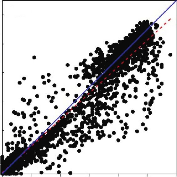
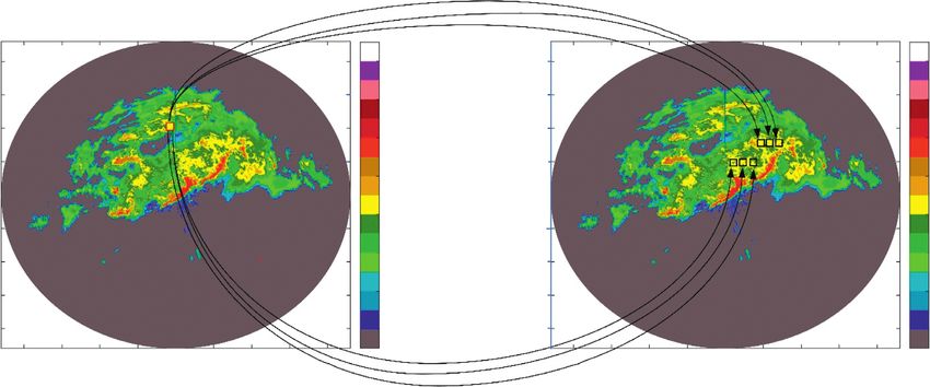
Scientific Programming 5

algorithm [25]. Denote by x the estimation of x and denote ai , if xi is an element of ηi , ai ∈ aki ,
by x i a local patch of x . For each x i , a subdictionary will be A(i, j) � (12)
 0, otherwise.
selected from dictionary set for reconstruction, which can be
completed in the subspace of U � [μ1 , μ2 . . . , μK ]. Apply Therefore, equation (11) can be rewritten as follows:
SVD to the covariance matrix of U including all the cen-
troids to get the PCA transformation matrix of U. Let Φc be a � arg min ‖y − DΦ ∘ a‖22 + λ · ‖a‖1 + ε · ‖(I − A)x‖22 .
 a
the projection matrix composed by the first several most
significant eigenvectors, the distance between μk and x i can (13)
be calculated in the subspace of Φc .
 �� ��
 ki � arg min ��Φc x i − Φc μk ��2. (9) 4.4. Adaptive Nonlocal Regularization. Statistics show that
 k
 the weather radar echo contains many repetitive structures
 By solving equation (9), subdictionary Φki is adaptively and shapes. As shown in Figure 3, the red box in the left
selected and assigned to echo patch x i , so we can update the plane position indicator (PPI) and the black box in the right
estimation ( x � Φ ∘ a) of x by minimizing equation (5). PPI indicate the given radar echo patch and the radar echo
 patches, that is, nonlocally similar to it, respectively; many
 similar and repetitive structures can be observed between
4.3. Adaptive Autoregressive Regularization. To ensure the two echo patches (for example, the reflectivity data of the
local stability of radar echo during the reconstruction first layer elevation angle of CINRAD-SA radar (10 : 36 (BJT)
process, we use spatial autoregressive (AR) regularization to on June 23, 2016). This has 360 radials, and each radial has
constrain the optimal solution of sparse coefficients and 460 range bins; this nonlocal redundant information has the
realizes the parameter adjustment of superresolution local effect of enhancing the sparse decomposition stability of
reconstruction. For each cluster Ck , an AR model can be weather radar echoes, improving the quality of weather
obtained by training the sample echo patches in the cluster. radar echo reconstruction. Therefore, this paper introduces
In the construction of the training model, too high an order the regularization constraint based on nonlocal (NL) sim-
may lead to data over fitting. Therefore, this article uses a ilarity to further improve the reconstruction effect.
window of 3 × 3, and the training order is 8. By solving the For each weather radar echo patch xi , search for similar
least square problem in the following formula, the AR model patches xli in the whole echo x. The criteria for screening xi
parameter vector of the Kth cluster can be calculated by are as follows:
 �� ��2
 ak � arg min pi − aT di , eli � ���xi − xli ��� ≤ t, (14)
 a
 (10) 2
 pi ∈Ck
 where t is the preset threshold and the linear representation
where pi is the center value of the weather radar echo patch coefficient is obtained by
pi and di is the column vector composed of eight sur- l
rounding data values. A series of AR model parameter −ei /h
 bli � exp . (15)
vectors a1 , a2 , . . . , aK can be obtained by equation (10). ci
 For each radar echo patch, an AR model is adaptively
selected from a1 , a2 , . . . , aK for reconstruction. The specific In equation (15), ci � l exp(−eli /h) is the normalization
selection scheme is the same as that of the subdictionary; let factor, h is the control term of weight, and the expected error
ki � arg min ‖Φc x i − Φc μk ‖2, then the ki AR model will be term is calculated by
 �� ��2
assignedk to patch xi . The autoregressive regularization �� � �� ��2
 � l l�
constraint is to solve the minimum error between the actual ���xi − bi xi ��� � ��xi − bTi βi ��2
 �
 xi ∈x � �2 xi ∈x (16)
value and the estimated value aTki ηi of the center of the radar l

echo patch xi , which is equivalent to minimizing
 2
 � ‖(I − B)x‖22 ,
‖xi − aTki ηi ‖2 and ηi denotes the column vector composed of 8
data values around xi . By adding the autoregressive regu- where xi denotes the central value of xi , xli denotes the
larization term as a local constraint to the solution process of central value of xli , and I is the identity matrix, and
the sparsity coefficient, the sparse vector is obtained by ⎨ bl ,
 ⎧ if xli is an element of ηi , bli ∈ bi
solving the following minimization problem: B(i, l) � ⎩ i (17)
 0, otherwise.
 ⎪
 ⎧
 ⎨ �� �⎫ ⎪
 a � arg min⎪‖y − DΦ ∘ a‖22 + λ · ‖a‖1 + ε · ��x − aT η ���2 ⎬ , Therefore, by incorporating the expected error term,
 ⎩ � i ki i �2 ⎪
 ⎭
 a x ∈xi i equation (5) can be improved as follows:
 (11) a � arg min ‖y − DΦ ∘ a‖22 + λ · ‖a‖1 +δ · ‖(I − B)x‖22 ,
 a
where ε is a constant that balances the constraint of AR (18)
regularization term. For convenience of expression, we re-
 2
write the third term xi ∈xi ‖xi − aTki ηi ‖2 as ‖(I − A)x‖22 , where where δ is a constant that balances the constraint of the NL
I is an identity matrix and regularization term.
6 Scientific Programming

 Reflectivity PPI (dBZ) Reflectivity PPI (dBZ)

 400 70 400 70
 300 60 300 60
 200 200
 50 50
 Distance (km)

 Distance (km)
 100 100
 40 40
 0 0
 30 30
 -100 -100
 20 20
 -200 -200
 -300 10 -300 10

 -400 0 -400 0
 -400 -300 -200 -100 0 100 200 300 400 -400 -300 -200 -100 0 100 200 300 400
 Distance (km) Distance (km)
 Figure 3: Example of a nonlocally similar echo patches.

4.5. Algorithm of ASDS. By combining local autoregressive (3) Parameter Settings: in the experiment, the original
(AR) regularization constraint and nonlocal (NL) self- echo data are used as the high-resolution (HR) radar
similar regularization constraint into equation (5), we obtain echo; the low-resolution radar echo can be obtained
a final sparse representation algorithm based on ASDS to through blurring, subsampling, and noise process-
reconstruct weather radar echo, which can be described as ing, where fuzzy kernel is a Gaussian kernel with size
 of 7 × 7 and standard deviation of 1.5, the sub-
 a � arg min ‖y − DΦ ∘ a‖22 + ε · ‖(I − A)Φ ∘ a‖22 +δ · sampling factors are 2 and 4, and the additive noise is
 a
 , (19) white noise. In addition, the initialization of the
 ‖(I − B)Φ ∘ a‖22 + λ · ‖a‖1 parameters in the ASDS algorithm is as follows: the
 number of subdictionaries obtained through K-PCA
where the second l2 norm is an adaptive regularization term is K � 200, and the regularization parameters of the
based on the local AR model, which ensures that the esti- sparse coefficient term, AR term, and NL term are
mated weather radar echo is locally stationary, and the third λ � 5, ε � 0.06, δ � 0.25, respectively. In dictionary
l2 norm is a nonlocal similar regularization term, which uses learning processes, the total amount of echo patches
nonlocal redundancy to enhance each local echo patch. The with a size of 7 × 7 is 16000. To find the optimal
algorithm flow of ASDS is shown in Algorithm 1. number of iterations, we calculated the PSNR values
 of the reflectivity data for different weather condi-
5. Implementation Details tions and down-sampling scales. As shown in Fig-
 (1) Data: the dictionary learning and performance ure 4, the optimal number of iterations is
 evaluation of the proposed ASDS algorithm is car- Max_Iter � 720 , and the iteration error is e � 2 ×
 ried out using the reflectivity data from S-band 10− 6 and P � 150.
 China’s new generation weather radar (CINRAD- (4) Evaluation metrics: to evaluate the effectiveness of
 SA), which include the precipitation experimental the proposed ASDS algorithm, we compare ASDS
 data of South China in Guangdong on May to June with bicubic and IFS interpolation in terms of visual
 2016, the tornado and hail data of Yancheng in quality and quantitative results. The peak-signal-to-
 Jiangsu on May 27, 2008, the tornado data of noise ratio (PSNR) (dB) and structural similarity
 Yancheng in Jiangsu on June 23, 2016, Nantong in (SSIM) [26] are used to quantitatively evaluate the
 Jiangsu on July 06, 2016, and the typhoon data of reconstruction effect.
 Xuzhou in Jiangsu in August 2018.
 (2) Degradation method: the weather radar echo deg- 6. Experimental Results and Analysis
 radation process includes three processes: blurring, In this section, we compare ASDS with bicubic and IFS in-
 down-sampling, and system noise. Degradation terpolation in terms of visual quality and quantitative results.
 process can be formulated by
 y � Dx + n, (20) 6.1. Visual Quality Comparison. The reflectivity data of the
 first elevation cut under precipitation (Heyuan, Guangdong,
 where D represents the degradation operation (e.g., China, 12 : 06, June 15, 2016) and typhoon (Xuzhou, Jiangsu,
 blurring kernel, down-sampling operation) and n China, 11 : 00, August 18, 2018) condition are selected to test
 represents the weather radar receiver noise, which the performance of ASDS under large-scale weather system
 obeys the zero-mean Gaussian distribution. and to compare it with bicubic and IFS interpolation.
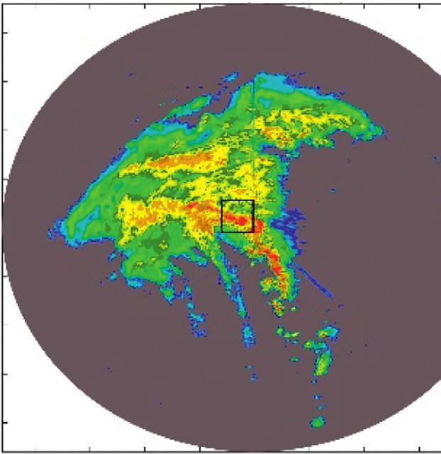
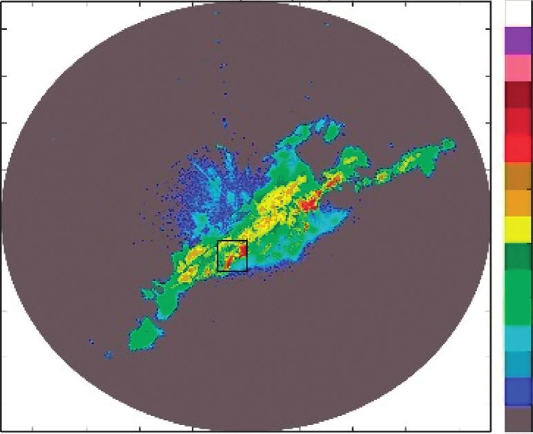
Scientific Programming 7

 38 35 33

 37.8 34.8 32.8

 ×4 PSNR(dB) of Small-scale Weather System

 ×4 PSNR(dB) of Large-scale Weather System
 ×4 PSNR(dB) of Cloudless

 37.6 34.6 32.6

 37.4 34.4 32.4

 37.2 34.2 32.2

 37 34 32
 0 120 240 360 480 600 720 840 960
 Number of Iterations
 Large-scale Weather System
 Small-scale Weather System
 Cloudless
 Figure 4: PSNR value of reconstructed reflectivity data under different weather conditions for ×4 downsampling.

 Require:
 Set the initial estimation x by using wavelet domain and the iterative threshold algorithm [25].
 Preset ε, δ, P, e and the maximal iteration number, denoted by Max_Iter and set k � 0
 2
 Ensure: Iterate on k until ‖ x(k) − x (k+1) ‖2 ≤ e or k ≥ Max_Iter
 (1) Select subdictionary Φki and AR model ai for each x i through equation (9) and calculate the nonlocal weight bi for each x i
 (2) Calculate A and B with the selected AR models and the non-local weights
 (3) Compute a(k+1)i through equation (19), which can be calculated by using iterative threshold algorithm. Then, we can get
 x i (k+1) � Φki a(k+1)
 i
 (4) Calculate x (k+1) by averaging all the reconstructed echo patches, which can be completed by equation (4)
 (5) If mod(k, P) � 0 update the adaptive sparse domain of and the matrices A and B using x (k+1) .

 ALGORITHM 1: Adaptive sparse domain selection (ASDS) algorithm.

 Intense precipitation convective cells are often embedded recovering intense echo information, it has lack in rebuilding
in a lower intensity region, which shows high aggregation and echo with more fine-grained structure. Compared with
sparse correlation. Therefore, capturing as much detailed bicubic and IFS interpolation, ASDS algorithm has better
information as possible about the intense echo can help in ability in recovering more of the fine-grained structure and is
operational research and forecast on intense precipitation. As notably better at preserving sharp edges associated with the
shown in the black box of Figure 5, it can be seen that under large-scale features. Under ×4 reconstruction, compared with
×2 reconstruction, the bicubic reconstructed radar echo lose the terrible performance of bicubic and IFS interpolation in
most of the intense echo information, resulting in overly recovering the detail information of radar echo, ASDS al-
smooth radar echo, which indicate that the simple interpo- gorithm is capable of recovering the edge and highlighting the
lation method using several neighboring data values for location of intense echo. As shown in the black box of Fig-
computational approximation to get the estimated value is not ure 6, the ASDS reconstructed echo is most similar to the
capable of being applied in intense precipitation condition. original echo and achieve the best subjective quality under
Although IFS interpolation performs better than bicubic in typhoon condition.
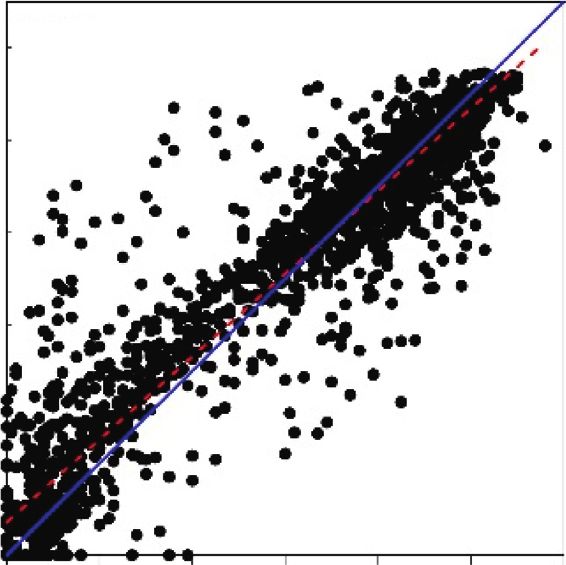
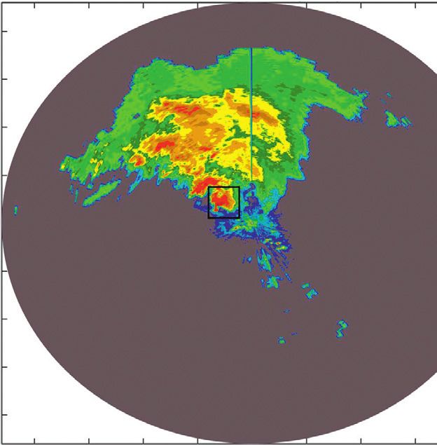
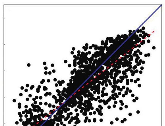
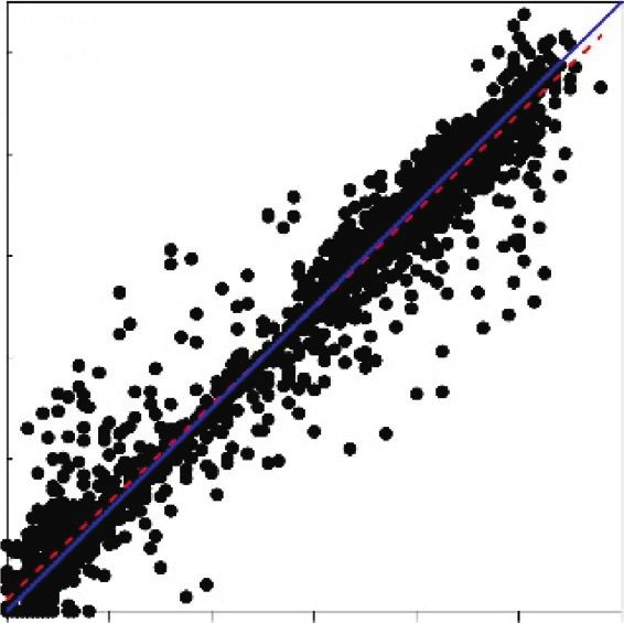
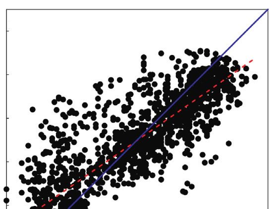
8 Scientific Programming

 Reflectivity PPI (dBZ)

 400 70

 300 60
 200
 50
 Distance (km)

 100
 40
 0 Ground truth ×2 Bicubic ×2 IFS ×2 ASDS
 30
 -100
 20
 -200

 -300 10

 -400 0

 -400 -300 -200 -100 0 100 200 300 400 Ground truth ×4 Bicubic ×4 IFS ×4 ASDS
 Distance (km)

 Figure 5: Visual comparison of superresolution reconstruction results of intense precipitation data.

 Reflectivity PPI (dBZ)

 400 70

 300 60
 200
 50
 Distance (km)

 100
 40
 0 Ground truth ×2 Bicubic ×2 IFS ×2 ASDS
 30
 -100

 -200 20

 -300 10

 -400 0
 -400 -300 -200 -100 0 100 200 300 400 Ground truth ×4 Bicubic ×4 IFS ×4 ASDS
 Distance (km)

 Figure 6: Visual comparison of superresolution reconstruction results of typhoon data.

 Tornado is an intense unstable weather condition of 6.2. Quantitative Results Comparison. Figure 8 shows the
small-scale convective vorticity, with a central wind speed of direct comparison between the estimated values and the
up to 100–200 m/s. A tornado cycle is short, usually only for a ground truth data in the cases corresponding to the ones
few minutes, with the longest not being more than a few showing in Figures 5–7. In Figure 8, the bicubic and IFS
hours, so tornado detection and early warning forecast are scatters are heavily distributed above the 1 : 1 diagonal in the
very difficult. Most of the tornadoes, especially, those above weak echo region (10–30/dBZ), that is, underestimation, and
EF-2 (Enhanced fujita) mainly occur in supercell storms heavily distributed above the 1 : 1 diagonal in the intense
[27, 28]. Hook echo is the area where tornadoes may occur in echo (40–60/dBZ) region, that is, overestimation. The scatter
supercell thunderstorms. Therefore, recovering as much de- of ASDS are mostly distributed near the 1 : 1 diagonal, which
tailed information as possible about the hook echo from indicates that the estimation of ASDS is better consistent
degraded weather radar echo can help in tornado detection with the ground truth, especially in the intense echo region.
and forecast. As shown in the black box of Figure 7, although Statistically speaking, ASDS has the better performance for
both the IFS interpolation and the ASDS algorithm can re- coefficient of determination (R2) than bicubic and IFS. To
cover most of the hook echo detail information under ×2 further validate the effectiveness of ASDS under different
reconstruction, the hook echo reconstructed by the ASDS weather condition (e.g., large- and small-scale weather
algorithm is closer to the ground truth. Under ×4 recon- system, cloudless), the statistical comparison is made in
struction, although all methods fail to recover the fine-grained terms of quantitative evaluation metrics (PSNR, SSIM). All
structure of hook echo, the ASDS algorithm has the better the results on ×2 and ×4 reconstruction are shown in Table 1,
performance in highlighting the location of intense echo. from which we can see that ASDS shows the best PSNR and
Scientific Programming 9

 Reflectivity PPI (dBZ)

 400 70

 300 60
 200
 50
 Distance (km)

 100
 40
 0 Ground truth ×2 Bicubic ×2 IFS ×2 ASDS
 30
 -100
 20
 -200

 -300 10

 -400 0

 -400 -300 -200 -100 0 100 200 300 400 Ground truth ×4 Bicubic ×4 IFS ×4 ASDS
 Distance (km)

 Figure 7: Visual comparison of superresolution reconstruction results of tornado data.

 60 60 60
 R2 = 0.89 R2 = 0.93 R2 = 0.97
 50 50 50

 40
 40 40
 ×2 IFS/dBZ
 ×2 Bicubic/dBZ

 ×2 ASDS/dBZ
 30
 30 30
 20
 20 20
 10
 10 10
 0
 0 0
 0 10 20 30 40 50 60 0 10 20 30 40 50 60 0 10 20 30 40 50 60
 Ground truth/dBZ Ground truth/dBZ Ground truth/dBZ

 60 60 60
 R2 = 0.73 R2 = 0.76 R2 = 0.88
 50 50 50

 40 40 40
 ×4 Bicubic/dBZ

 ×4 ASDS/dBZ
 ×4 IFS/dBZ

 30 30 30

 20 20 20

 10 10 10

 0 0 0
 0 10 20 30 40 50 60 0 10 20 30 40 50 60 0 10 20 30 40 50 60
 Ground truth/dBZ Ground truth/dBZ Ground truth/dBZ

 (a)
 Figure 8: Continued.
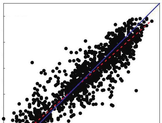
10 Scientific Programming

 60 60 60
 2
 R = 0.88 R2 = 0.89 R2 = 0.93
 50 50 50

 40 40 40
 ×2 Bicubic/dBZ

 ×2 ASDS/dBZ
 ×2 IFS/dBZ
 30 30 30

 20 20 20

 10 10 10

 0 0 0
 0 10 20 30 40 50 60 0 10 20 30 40 50 60 0 10 20 30 40 50 60
 Ground truth/dBZ Ground truth/dBZ Ground truth/dBZ

 60 60 60
 2
 R = 0.79 R2 = 0.72 R2 = 0.84
 50 50 50

 40 40 40
 ×4 Bicubic/dBZ

 ×4 ASDS/dBZ
 ×4 IFS/dBZ

 30 30 30

 20 20 20

 10 10 10

 0 0 0
 0 10 20 30 40 50 60 0 10 20 30 40 50 60 0 10 20 30 40 50 60
 Ground truth/dBZ Ground truth/dBZ Ground truth/dBZ

 (b)
 60 60 60
 R2 = 0.95 R2 = 0.96 R2 = 0.99
 50 50 50

 40 40 40
 ×2 Bicubic/dBZ

 ×2 ASDS/dBZ
 ×2 IFS/dBZ

 30 30 30

 20 20 20

 10 10 10

 0 0 0
 0 10 20 30 40 50 60 0 10 20 30 40 50 60 0 10 20 30 40 50 60
 Ground truth/dBZ Ground truth/dBZ Ground truth/dBZ

 60 60 60
 2
 R = 0.87 R2 = 0.90 R2 = 0.96
 50 50 50

 40 40 40
 ×4 Bicubic/dBZ

 ×4 ASDS/dBZ
 ×4 IFS/dBZ

 30 30 30

 20 20 20

 10 10 10

 0 0 0
 0 10 20 30 40 50 60 0 10 20 30 40 50 60 0 10 20 30 40 50 60
 Ground truth/dBZ Ground truth/dBZ Ground truth/dBZ

 (c)

Figure 8: Scatter plot and fitted curve corresponding to the cases showing in Figures 5–7. The X-axis denotes the ground truth, and Y-axis
denotes the estimation by different methods. (a) Intense precipitation. (b) Typhoon. (c) Tornado.
Scientific Programming 11

 Table 1: Quantitative results of the compared methods on different weather condition.
 ASDS
 Bicubic IFS ASDS (AR) ASDS (NL)
Weather condition Scale (AR + NL)
 PSNR SSIM PSNR SSIM PSNR SSIM PSNR SSIM PSNR SSIM
Large-scale weather system ×2 31.59 0.9102 34.23 0.9225 35.21 0.9239 35.46 0.9215 35.61 0.9382
Small-scale weather system ×2 33.07 0.9215 35.85 0.9391 36.87 0.9425 36.98 0.9431 37.34 0.9437
Cloudless ×2 34.94 0.9287 36.91 0.9446 38.56 0.9518 38.74 0.9527 39.21 0.9613
Large-scale weather system ×4 28.81 0.8428 31.25 0.8792 32.66 0.8945 32.87 0.8967 33.11 0.9021
Small-scale weather system ×4 30.16 0.9122 32.97 0.9098 34.63 0.9012 34.78 0.9085 34.92 0.9146
Cloudless ×4 32.18 0.9082 34.87 0.9121 35.86 0.9318 36.12 0.9269 36.22 0.9328
The best results are in bold.

SSIM in all weather conditions, with PSNR is even more than References
2 dB higher than bicubic interpolation. We can also see that
ASDS with NL regularization produces subjectively superior [1] D. B. McRoberts and J. W. Nielsen-Gammon, “Detecting
results than with AR regularization, indicating promising beam blockage in radar-based precipitation estimates,”
 Journal of Atmospheric and Oceanic Technology, vol. 34, no. 7,
performance of exploiting nonlocal correlation information
 pp. 1407–1422, 2017.
of weather radar echo. [2] J. M. Schmidt, P. J. Flatau, P. R. Harasti et al., “Radar detection
 of individual raindrops,” Bulletin of the American Meteoro-
7. Conclusion logical Society, vol. 100, no. 12, pp. 2433–2450, 2019.
 [3] C. D. Curtis and S. M. Torres, “Adaptive range oversampling
Different from the interpolation methods, this method only to improve estimates of polarimetric variables on weather
utilizes the neighboring information. In this article, we radars,” Journal of Atmospheric and Oceanic Technology,
propose the ASDS algorithm for superresolution recon- vol. 31, no. 9, pp. 1853–1866, 2014.
struction of weather radar data, which effectively exploit the [4] S. M. Torres and C. D. Curtis, “The impact of range-over-
sparsity and local and nonlocal characteristics of weather sampling processing on tornado velocity signatures obtained
radar data by introducing sparse, local, and nonlocal reg- from WSR-88D superresolution data,” Journal of Atmospheric
 and Oceanic Technology, vol. 32, no. 9, pp. 1581–1592, 2015.
ularization. Experimental results show that the ASDS al-
 [5] S. M. Torres and C. D. Curtis, “Revisiting the optimum re-
gorithm substantially outperforms interpolation methods ceiver filter bandwidth for range-oversampling processing,”
for ×2 and ×4 rebuilding in terms of both visual quality and Journal of Atmospheric and Oceanic Technology, vol. 37, no. 3,
quantitative evaluation metrics. Although we use the K-PCA pp. 507–515, 2020.
algorithm to obtain the compact dictionary from the [6] W. T. Freeman, T. R. Jones, and E. C. Pasztor, “Example-
training set in advance instead of updating the dictionary based super-resolution,” IEEE Computer graphics and Ap-
during each iteration, which can greatly reduce the time plications, vol. 22, no. 2, pp. 56–65, 2002.
required for superresolution reconstruction, the ASDS al- [7] S. S. Weygandt, A. Shapiro, and K. K. Droegemeier, “Retrieval
gorithm still has a large amount of computation. With the of model initial fields from single-Doppler observations of a
increasing demand for extreme weather warning and supercell thunderstorm. part i: single-Doppler velocity re-
forecast, the ASDS algorithm still has a lot of room for trieval,” Monthly Weather Review, vol. 130, no. 3, pp. 433–453,
optimization. 2002.
 [8] E. Ruzanski and V. Chandrasekar, “Weather radar data in-
 terpolation using a kernel-based Lagrangian nowcasting
Data Availability technique,” IEEE Transactions on Geoscience and Remote
 Sensing, vol. 53, pp. 3073–3083, 2014.
The datasets used during the current study are available from [9] E. Sharifi, B. Saghafian, and R. Steinacker, “Downscaling
the corresponding author on reasonable request. satellite precipitation estimates with multiple linear regres-
 sion, artificial neural networks, and spline interpolation
Conflicts of Interest techniques,” Journal of Geophysical Research: Atmospheres,
 vol. 124, no. 2, pp. 789–805, 2019.
The authors declare that there are no conflicts of interest. [10] L. Kou, Y. Jiang, A. Chen, and Z. Wang, “Statistical modeling
 with a hidden Markov tree and high-resolution interpolation
 for spaceborne radar reflectivity in the wavelet domain,”
Acknowledgments Advances in Atmospheric Sciences, vol. 37, no. 12, pp. 1359–
 1374, 2020.
This work was supported by the National Key R&D Program [11] M. Ebtehaj and E. Foufoula-Georgiou, “Statistics of precipi-
of China (2018YFC01506100), the http://dxNational Natural tation reflectivity images and cascade of Gaussian-scale
Science Foundation of China (U20B2061), and the http:// mixtures in the wavelet domain: a formalism for reproducing
dxDepartment of Science and Technology of Sichuan extremes and coherent multiscale structures,” Journal of
Province (2020ZYD051). Geophysical Research: Atmospheres, vol. 116, 2011.
12 Scientific Programming

[12] E. Foufoula-Georgiou, A. M. Ebtehaj, S. Q. Zhang, and [28] A. K. Anderson-Frey, Y. P. Richardson, A. R. Dean,
 A. Y. Hou, “Downscaling satellite precipitation with emphasis R. L. Thompson, and B. T. Smith, “Characteristics of tornado
 on extremes: a variational ℓ1-norm regularization in the events and warnings in the southeastern United States,”
 derivative domain,” The Earth’s Hydrological Cycle, vol. 35, Weather and Forecasting, vol. 34, no. 4, pp. 1017–1034, 2019.
 pp. 765–783, 2013.
[13] A. M. Ebtehaj and E. Foufoula-Georgiou, “On variational
 downscaling, fusion, and assimilation of hydrometeorological
 states: a unified framework via regularization,” Water Re-
 sources Research, vol. 49, no. 9, pp. 5944–5963, 2013.
[14] A. M. Ebtehaj, E. Foufoula-Georgiou, and G. Lerman, “Sparse
 regularization for precipitation downscaling,” Journal of
 Geophysical Research: Atmospheres, vol. 117, 2012.
[15] X. Zhang, J. He, Q. Zeng, and Z. Shi, “Weather radar echo
 super-resolution reconstruction based on nonlocal self-sim-
 ilarity sparse representation,” Atmosphere, vol. 10, no. 5,
 p. 254, 2019.
[16] M. Xu, Q. Liu, D. Sha et al., “Precipatch: a dictionary-based
 precipitation downscaling method,” Remote Sensing, vol. 12,
 no. 6, p. 1030, 2020.
[17] H. Yuan, Q. Zeng, and J. He, “Adaptive regularized sparse
 representation for weather radar echo super-resolution re-
 construction,” in Proceedings of the 2021 International Con-
 ference on Electronic Information Engineering and Computer
 Science (EIECS), pp. 33–38, Changchun, China, 2021
 September.
[18] S. McCarroll, M. Yeary, D. Hougen, V. Lakshmanan, and
 S. Smith, “Approaches for compression of super-resolution
 WSR-88D data,” IEEE Geoscience and Remote Sensing Letters,
 vol. 8, pp. 191–195, 2010.
[19] Q. Zeng, J. He, Z. Shi, and X. Li, “Weather radar data
 compression based on spatial and temporal prediction,” At-
 mosphere, vol. 9, no. 3, p. 96, 2018.
[20] T. Wang, R. Jobredeaux, M. Pantel, P.-L. Garoche, E. Feron,
 and D. Henrion, “Credible autocoding of convex optimization
 algorithms,” Optimization and Engineering, vol. 17, no. 4,
 pp. 781–812, 2016.
[21] E. Nozari, P. Tallapragada, and J. Cortés, “Differentially
 private distributed convex optimization via functional per-
 turbation,” IEEE Transactions on Control of Network Systems,
 vol. 5, pp. 395–408, 2016.
[22] T. Huang, W. Dong, X. Xie, G. Shi, and X. Bai, “Mixed noise
 removal via Laplacian scale mixture modeling and nonlocal
 low-rank approximation,” IEEE Transactions on Image Pro-
 cessing, vol. 26, no. 7, pp. 3171–3186, 2017.
[23] D. Li, X. Tian, Q. Jin, and K. Hirasawa, “Adaptive fractional-
 order total variation image restoration with split Bregman
 iteration,” ISA Transactions, vol. 82, pp. 210–222, 2018.
[24] B. Shi, Z.-F. Pang, and J. Wu, “Alternating split Bregman
 method for the bilaterally constrained image deblurring
 problem,” Applied Mathematics and Computation, vol. 250,
 pp. 402–414, 2015.
[25] N. Zarmehi and F. Marvasti, “Sparse and low-rank recovery
 using adaptive thresholding,” Digital Signal Processing,
 vol. 73, pp. 145–152, 2018.
[26] Z. Wang, A. C. Bovik, H. R. Sheikh, and E. P. Simoncelli,
 “Image quality assessment: from error visibility to structural
 similarity,” IEEE Transactions on Image Processing, vol. 13,
 no. 4, pp. 600–612, 2004.
[27] R. S. Schumacher, D. T. Lindsey, A. B. Schumacher, J. Braun,
 S. D. Miller, and J. L. Demuth, “Multidisciplinary analysis of
 an unusual tornado: meteorology, climatology, and the
 communication and interpretation of warnings∗,” Weather
 and Forecasting, vol. 25, no. 5, pp. 1412–1429, 2010.
You can also read