Global field reconstruction from sparse sensors with Voronoi tessellation-assisted deep learning
←
→
Page content transcription
If your browser does not render page correctly, please read the page content below
Global field reconstruction from sparse sensors with
                                                   Voronoi tessellation-assisted deep learning
                                                   Kai Fukami1,2,* , Romit Maulik3 , Nesar Ramachandra4 ,
                                                   Koji Fukagata2 , and Kunihiko Taira1
                                                   1 Department of Mechanical and Aerospace Engineering, University of California, Los Angeles
                                                   2 Department of Mechanical Engineering, Keio University
                                                   3 Argonne Leadership Computing Facility, Argonne National Laboratory
arXiv:2101.00554v2 [physics.flu-dyn] 22 Jul 2021

                                                   4 High Energy Physics Division, Argonne National Laboratory
                                                   * kfukami1@g.ucla.edu

                                                   ABSTRACT

                                                   Achieving accurate and robust global situational awareness of a complex time-evolving field from a limited number of sensors
                                                   has been a longstanding challenge. This reconstruction problem is especially difficult when sensors are sparsely positioned in
                                                   a seemingly random or unorganized manner, which is often encountered in a range of scientific and engineering problems.
                                                   Moreover, these sensors can be in motion and can become online or offline over time. The key leverage in addressing this
                                                   scientific issue is the wealth of data accumulated from the sensors. As a solution to this problem, we propose a data-driven
                                                   spatial field recovery technique founded on a structured grid-based deep-learning approach for arbitrary positioned sensors
                                                   of any numbers. It should be noted that the naïve use of machine learning becomes prohibitively expensive for global field
                                                   reconstruction and is furthermore not adaptable to an arbitrary number of sensors. In the present work, we consider the use of
                                                   Voronoi tessellation to obtain a structured-grid representation from sensor locations enabling the computationally tractable use
                                                   of convolutional neural networks. One of the central features of the present method is its compatibility with deep-learning based
                                                   super-resolution reconstruction techniques for structured sensor data that are established for image processing. The proposed
                                                   reconstruction technique is demonstrated for unsteady wake flow, geophysical data, and three-dimensional turbulence. The
                                                   current framework is able to handle an arbitrary number of moving sensors, and thereby overcomes a major limitation with
                                                   existing reconstruction methods. The presented technique opens a new pathway towards the practical use of neural networks
                                                   for real-time global field estimation.

                                                   1 Introduction
                                                   Spatial field reconstruction from limited local sensor information is a major challenge in the analysis, estimation, control, and
                                                   design of high-dimensional complex physical systems. For complex physics including geophysics1 , astrophysics2 , atmospheric
                                                   science3, 4 , and fluid dynamics5 , traditional linear theory-based tools, including Galerkin transforms6, 7 , linear stochastic
                                                   estimation8, 9 and Gappy proper orthogonal decomposition10 , have faced challenges in reconstructing global fields from a
                                                   limited number of sensors. Neural networks have emerged as hopeful nonlinear alternatives to reconstruct chaotic data from
                                                   sparse measurements in an efficient manner11, 12 . However, there are key limitations associated with neural networks for field
                                                   reconstruction. One of the biggest difficulties is the applicability of neural network-based methods to unstructured grid data.
                                                   Almost all practical experimental measurements or numerical simulations rely on unstructured grids or non-uniform/random
                                                   sensor placements. These grids are not compatible with convolutional neural network (CNN)-based methods which are founded
                                                   on training data being structured and uniformly arranged13, 14 . While a multi-layer perceptron (MLP)15 can handle unstructured
                                                   data, its use is sometimes impractical due to their globally connected network structure. Moreover, MLPs cannot handle sensors
                                                   that may go offline or move in space. On the other hand, graph convolutional networks (GCNs) have been utilized to perform
                                                   convolutions on unstructured data16 . However, GCNs are also known to scale poorly and their state-of-the-art applications have
                                                   been limited to the order of 105 degrees of freedom17 . Even such applications of GCNs have required distributed learning on
                                                   several hardware accelerators. This restricts their utilities for practical field reconstructions. A greater limitation stems from
                                                   the fact that all methods fail to handle spatially moving sensors. This implies that applications of these conventional tools
                                                   are limited to a fixed sensor arrangement as that used in a training process. This limitation is a major hindrance to practical
                                                   use of these reconstruction techniques, since experimental sensor locations commonly evolve over time. The framework that
                                                   integrates convolutional architectures with time-varying unstructured data is crucial for bridging the gap between structured
                                                   field reconstructions and practical problems18 .
                                                       In response to the aforementioned challenges, we propose a method that incorporates sparse sensor data into a CNN by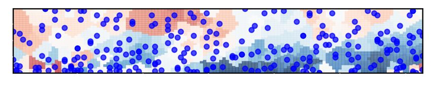
Voronoi image construction                                     Deep learning based global field reconstruction
            s8
            …

      s3                                                                 Convolutional neural network
  s2                                        Mask image
 s1

                                 t

                                                                                                            …
                                                                              …

                                                                                           …
                 s3             s7
            s2             s6
                  s4
       s1                 s5    s8                                                                …
                                          Voronoi image

Figure 1. Voronoi tessellation aided global data recovery from discrete sensor locations for a two-dimensional cylinder wake.
Input Voronoi image is constructed from 8 sensors. The Voronoi image is then fed into a convolutional neural network with the
mask image. In the mask image, a grid having a sensor (blue circle) has 1 while otherwise 0.

approximating the local information onto a structured representation, while retaining the information of spatial sensor locations.
This is achieved by constructing a Voronoi tessellation of the unstructured data set and adding the input data field corresponding
to spatial sensor locations through a mask. Voronoi tessellation projects local sensor information onto the structured-grid
field based on the Euclidean distance. The currently technique achieves accurate field reconstructions from arbitrary sensor
locations and varying numbers of sensors with existing CNN architectures. The present formulation will impact a wide range of
research fields that rely on fusing information from discrete sensors, e.g, buoy-based sensors and tracers in particle tracking
velocimetry19 .

2 Problem setup and approach
Our objective is to reconstruct a two-dimensional global field variable q ∈ Rnx ×ny from local sensor measurements s ∈ Rn at
locations x s i ∈ R2 , i = 1, . . . , n. Here, nx and ny respectively denote the number of grid points in the horizontal and vertical
directions on a high-resolution field, and n indicates the number of local sensor measurements. The challenge here is to handle
arbitrary numbers of sensors at any locations over the field. The number of sensors can be changed in time and the sensors can
be moving. The reconstruction process should be performed with only a single machine learning model to avoid retraining
when sensors move or change their numbers.
    To achieve the goal of the present study, we utilize two input data files (images) for the CNN:
      1. Local sensor measurements projected on Voronoi tessellation sV = sV (ss) ∈ Rnx ×ny .
      2. Mask image sm = sm ({xxs i }ni=1 ) ∈ Rnx ×ny which contains the local sensors positions, defined as
                                   (
                           n        1 if x = x s i for any i,
              s m ({xxs i }i=1 ) =
                                    0 otherwise.

The two input images above are provided to a machine learning model F such that q = F (ssV , s m ) ∈ Rnx ×ny , where q is the
desired high-resolution field. With these two input vectors holding magnitude and position information of the sensors, the
present idea can deal with arbitrary sensor locations and arbitrary numbers of sensors. It should be noted that reconstruction
cannot be achieved with conventional methods, including MLPs and CNNs due to their structural constraints. In what follows,
we introduce Voronoi tessellation and machine learning framework, which are the two key components in the present approach.1

2.1 Voronoi tessellation
To use a machine learning framework, the sensor data needs to be projected into an image file in an appropriate manner.
Voronoi tessellation20 is a simple and spatially optimal projection of local sensor measurements onto the spatial domain. This
tessellation approach optimally partitions a given space E into n regions G = {g1 , g2 , ..., gn } using boundaries determined by
distances d among n number of sensors s21 . Using a distance function d, Voronoi tessellation can be expressed as
             gi = {si ∈ E|d(si , gi ) < d(si , g j ), j 6= i}.                                                                   (1)
      1 Sample   codes are available on https://github.com/kfukami/Voronoi-CNN.

                                                                                                                                2/10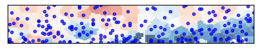
Hence, for a Euclidean domain, the Voronoi boundaries between sensors are their bisectors.
    Voronoi tessellation has two important characteristics which provide the foundation for the present approximation con-
structed with local sensor measurements21 . One is that each area in a Voronoi tessellation is convex. This property enables us
to establish a Voronoi tessellation using bisections in a simple manner. The other is that a Voronoi tessellation does not include
other sensors inside it when a circle centered at the vertex of a Voronoi region g passes neighboring sensors (Empty-circle
property). This implies that each Voronoi region g is optimal for each sensor s in a Voronoi tessellation. Note that the Voronoi
discretization is influenced by the computational domain size. Experimental setups are also influenced in analogous manner
with their finite fields of view. Additional details on the mathematical theory of Voronoi tessellation can be seen in the study of
Aurenhammer21 .
    The spatial domains to be discretized by Voronoi tessellation and the high-resolution data are taken to be the same size. All
grid points in each portion of the Voronoi image have its representative sensor value. Since Voronoi tessellation provides a
structured-grid representation of measurements from arbitrary placed sensors, the present approach enables us to use existing
CNNs devised for structured grid data. Note that a Voronoi tessellation needs to be performed solely once if sensors are
stationary. If the number of sensors change over time, only local regions in direct vicinity of added or removed sensors need to
undergo tessellation in an adaptive manner.

2.2 Convolutional neural network
The aforementioned Voronoi tessellation enables the use of deep learning through a structured-grid CNN13, 14, 22 . Our CNN
design is composed of convolutional layers as shown in figure 1. The convolutional layer extracts key features of input data
through filtering operations,
                                                     !
                   K−1 H−1 H−1
        (l)                        (l−1)
      qi jm = ψ    ∑ ∑ ∑ qi+p−C, j+c−C,k h pckm + bm          ,                                                                     (2)
                   k=0 p=0 c=0

                           (l−1)           (l)
where C = floor(H/2), qi jm and qi jm are the input and output data at layer l, respectively; h pckm represents a filter of size of
(H × H × K) and bm is the bias. In this study, the number of channels K is set to 1. The number of layers lmax , the size of filter
H, and the number of filter m are set to 9, 7, and 48, respectively, for the present study. The output of each filter operation is
passed through an activation function ψ which is chosen to be the rectified linear unit (ReLU) ψ(z) = max(0, z)23 . Moreover,
the ADAM optimizer24 is utilized with an early stopping criterion25 for the training process, which undergoes a three-fold
cross validation26 . Error are assessed using the L2 norm and ensemble evaluations. The present idea can also be extended to
three-dimensional problems without difficulty.
    For the input to F , we provide the Voronoi tessellation sV ∈ Rnx ×ny for sensor readings, with a mask image for input sensor
placements sm ∈ Rnx ×ny , i.e., q(0) = {ssv , sm } ∈ Rnx ×ny ×2 . The output from the CNN is a high-resolution flow field q ∈ Rnx ×ny ×1
that corresponds to the global field. In summary, the learning process of the present CNN can mathematically be formulated as
      w = argminw ||qq − F ({ssV , sm }; w)||2 ,                                                                                    (3)

where w denotes weights (filters) of CNN. We are now able to take measurements and locations by projecting them onto
Voronoi tessellation sV and the mask image sm , and reconstruct the global field variable q with deep learning F .

3 Applications
We demonstrate the use of the present Voronoi-based CNN for global fluid flow reconstruction. Our examples include laminar
cylinder wake, geophysical data, and three-dimensional wall-bounded turbulence, which contain strong nonlinear dynamics
over a wide range of spatio-temporal scales.

3.1 Example 1: two-dimensional cylinder wake
We first consider the Voronoi-based fluid flow reconstruction for a two-dimensional unsteady laminar cylinder wake at a
diameter-based Reynolds number ReD = 100. The training data set is prepared with a direct numerical simulation (DNS)27, 28
which numerically solves the incompressible Navier–Stokes equations. In this study, we consider the flow field data around a
cylinder body for the training and demonstration, i.e., ((x/D)∗ , (y/D)∗ ) = [−0.7, 15] × [−5, 5] and (Nx , Ny ) = (192, 112). The
vorticity field is used for both input and output attributes to the CNN model in this case. The training data spans approximately
4 vortex shedding periods. We examine the dependence of the reconstruction on the amount of training data. The number of
sensors nsensor is set to 8 and 16 with fixed input sensor locations for both training and testing.
    The reconstructed fields are shown in figure 2. The reconstructed vorticity fields are in excellent agreement comparing
to the reference vorticity field ω and in terms of the L2 error norm ε = ||ωref − ωML ||2 /||ωref ||2 , where ωref and ωML denote

                                                                                                                                  3/10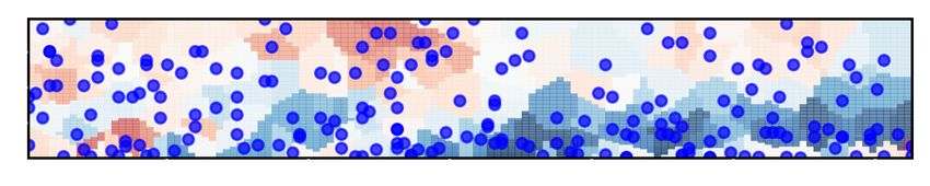
Voronoi input Mask (a)
(a)
(c)
nsensor = 8
Reference
(b)
-1.0 -0.5 0 0.5 1.0
(b)
nsensor = 16
(d)
(c)
(d)
nsnapshot
Figure 2. Voronoi-tessellation aided spatial data recovery of a two-dimensional cylinder wake with nsensor = 8 and 16. The
input Voronoi image, input mask image holding sensor locations, and the reconstructed vorticity field are shown. Dependence
of the reconstruction ability on the number of training snapshots is also shown. (a) {nsensor , nsnapshot } = {8, 50},
(b) {nsensor , nsnapshot } = {16, 50}, (c) {nsensor , nsnapshot } = {8, 5000}, and (d) {nsensor , nsnapshot } = {16, 5000}.
the reference and the reconstructed vorticity fields, respectively. It can be seen from the reconstructed vorticity field that the
vortices and shear layers in the near and far wakes are provided by the present deep learning technique with great accuracy and
detail. The vorticity field for nsensor = 8 shows some low-level reconstruction error due to the low number of sensors. When
nsensor is doubled to 16, we observe the error in the reconstruction is reduced by half with accurate recovery of the global flow
field. Furthermore, reasonable data recovery can be achieved with nsensor = 16 using as few as 50 training snapshots.
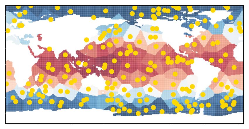
3.2 Example 2: NOAA sea surface temperature
Next, let us consider the NOAA sea surface temperature data collected from satellite and ship-based observations (http:
//www.esrl.noaa.gov/psd/). The data is comprised of weekly observations of the sea surface temperature with
a spatial resolution of 360 × 180. We use 1040 snapshots spanning from 1981 to 2001, while the test snapshots are taken
from 2001 to 2018. For this example, we take the sensors to be placed randomly over the water. The number of sensors for
training is set to nsensor,train = {10, 20, 30, 50, 100} with 5 different arrangements of sensor locations, amounting to 25 cases.
The sensor locations are randomly provided for each snapshot. For the test data, we also consider unseen cases with 70 and 200
sensors such that nsensor,test = {10, 20, 30, 50, 70, 100, 200}. These numbers of sensors for the test data correspond to {0.0154%,
0.0309%, 0.0463%, 0.0772%, 0.108%, 0.154%, 0.309%} against the number of grid points over the field. Both seen and unseen
sensor locations for all numbers of sensors are considered for the present test demonstrations. We emphasize that only a single
machine learning model is trained and used for all combinations of sensor numbers and sensor placements.
Let us demonstrate the global sea surface temperature reconstruction in figure 3. As a test case, we use a low nsensor = 30.
The reconstructed global temperature field by the present model shows great agreement with the reference data. This figure
also reports the L2 error norm ε = ||Tref − TML ||2 /||Tref ||2 , where Tref and TML are respectively the reference and reconstructed
temperature fields. We here also compare our results to standard linear and cubic interpolation. Since those are simple methods,
fine structures cannot be recovered and the L2 errors are larger than that of the present method. These trends are noticeable from
comparing the zoomed-in temperature contours. The interpolation schemes are unable to reconstruct the fine-grained features of
the temperature fields accurately. However, the proposed technique performs very well. In addition to enhanced reconstruction,
the present method is able to recover the whole field, while classical interpolation methods cannot extrapolate beyond the
convex hull covered by the sensors, as evident from figure 3. This observation also speaks to the significant advantage of the
present model.
Reference ML reconstruction Linear interpolation Cubic interpolation
Error: 0.0617 Error: 0.252 Error: 0.245
0 5 10 15 20 25 30
(℃)
Figure 3. Comparison of spatial data recovery for NOAA sea surface temperature with nsensor = 30.
4/10
Trained placement                     Unseen placement                          Unseen number of sensors
               Input
    nsensor= 100

                                              nsensor= 100

                                                                                        nsensor= 70
 CNN

                                                                                        nsensor= 200
Figure 4. Voronoi based spatial data recovery of NOAA sea surface temperature. We show the representative reconstructed
fields with nsensor = 100 which corresponds to the number of sensors contained in the training data and nsensor = {70, 200}
which correspond to cases not available in the training data set.

    Next, let us assess how the current approach performs when the number of sensors are changed and when the sensors are in
motion. We present the results for these cases in figure 4. With nsensor = 100 being the number of sensors observed during
training, the reconstructed sea surface temperature field is in agreement with the reference field for both trained (left) and
unseen sensor (middle) placements. Cases of unseen placements correspond to instances of sensors coming online or offline
during development and being in motion. Despite that the input Voronoi tessellation being significantly modified with the
displaced sensors, the reconstruction is still successful. This highlights the effective use of the mask image holding information
on sensor locations. What is also noteworthy is that successful reconstructions can be achieved with nsensor = 70 and 200,
which are numbers of sensors unseen during training. This corresponds to situations where sensors may come online or go
offline during deployment.
    The relationship between the number of input sensors and the L2 error norm is also investigated. The error level of the
test data with unseen placements (orange curve) is higher than that with trained placements (blue curve) as shown in figure 4.
However, the present model achieves a reasonable estimation with an L2 error being less than 0.1, even when the number of
unseen sensors reaches 200. This result suggests that the present approach employing the Voronoi input and the mask image
is robust for data sets where the number of sensors and the sensor placements vary considerably. It also demonstrates the
advantage of the present idea that a single trained model alone can handle the global field reconstruction for arbitrary number
of sensors and time-varying positions.

3.3 Example 3: turbulent channel flow
The above two problems contain strong periodicity in time, appearing as periodic vortex shedding and seasonal periodicity.
To further challenge the present approach, let us consider a chaotic and dynamically rich phenomenon of turbulent channel
flow. The flow field data is obtained by a direct numerical simulation of incompressible flow in a channel at a friction Reynolds
number of Reτ = 180. Here, x, y, and z directions are taken to be the streamwise, wall-normal, and spanwise directions. The size

                                                                                                                                  5/10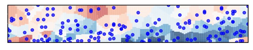
Reference

                              -4     -2     0      2     4
                                   Trained placement                                  Unseen placement
                                       nsensor = 200                                      nsensor = 200
                Input
                CNN

                                                        Unseen number of sensors
                                       nsensor = 150                                      nsensor = 250
                Input
                CNN

Figure 5. Voronoi tessellation-aided data recovery of turbulent channel flow. Considered are x − y cross sections of
streamwise velocity fluctuation u0 reconstructed with nsensor = 200 (trained number of sensors) and nsensor = {150, 250}
(untrained number of sensors). The error convergence over nsensor is also shown.

of the computational domain and the number of grid points are (Lx , Ly , Lz ) = (4πδ , 2δ , 2πδ ) and (Nx , Ny , Nz ) = (256, 96, 256),
respectively, where δ is the half width of the channel. Details of the simulation can be found in Fukagata et al.29 . For the
present study, x − y section of a subspace is used for the training process, i.e., x, y ∈ [0, 2πδ ] × [0, δ ] with (Nx∗ , Ny∗ ) = (128, 48).
The extracted subdomain maintains the same turbulent characteristics of the channel flow over the original domain, due to the
symmetry of statistics in the y direction and homogeneity in the x direction22 . We consider here the fluctuating component
of an x − y sectional streamwise velocity u0 as the variable of interest. For training, we use nsnapshot = 10 000. The numbers
of sensors for training data are chosen to be nsensor,train = {50, 100, 200} with 5 different cases of sensor placements. For
the test data, we also consider the use of 150 and 250 sensors with both trained and untrained sensor placements such that
nsensor,test = {50, 100, 150, 200, 250}. This setting allows us to assess the robustness of our approach for varied numbers of
sensor inputs analogous to Example 2, with consideration of both seen and unseen sensor locations for all numbers of sensors.
    The performance of Voronoi-assisted CNN-based spatial data recovery for turbulent channel flow is summarized in figure 5
for nsensor = {150, 200, 250}. These numbers of sensors amount to 2.44%, 3.26%, and 4.07% with respect to the number
of grid points over the field. We observe that finer flow features can be accurately reconstructed from just 200 sensors
indicating a remarkable degree of sparsity in measurement. Although error levels for unseen placement (i.e., the same number
of sensors but at different locations) is higher than that for trained sensor placement, similar trends are obtained. Notably,
reasonable reconstruction for both unseen number of sensors and unseen input sensor placement as shown in the results for
nsensor = {150, 250}. As these results suggest, the present approach is a powerful tool for global reconstruction of complex
flow fields from sparse sensor measurements.
    To quantitatively analyze reconstructed flow field, we examine the root-mean-square of the streamwise velocity fluctuations,
as shown in figure 6. The peak in the near-wall region and profile are captured well for all considered numbers of sensors. The
underestimations against the reference DNS curve are likely due to the use of fluctuation components and the use of an L2
minimization during the training process22, 30 . Since the supervised model minimizes a loss function through a training process,
the machine learning model tends to provide solution near the average value of training data to reduce the loss function. This
implies that the present machine learning model underestimates the fluctuations. Note that this is due to the supervised machine
learning framework and is not an issue imposed by the unstructured grid placements or the use of Voronoi tessellation. This
issue can be mitigated by using a loss function augmentation to the data, such as through z-scoring.
    To further assess the practical application of the present model, we analyze the effect of input noise on reconstruction. Here,
we consider the influence of two types of perturbations to the training data. Case I: Add noise to local sensor measurements sm

                                                                                                                                      6/10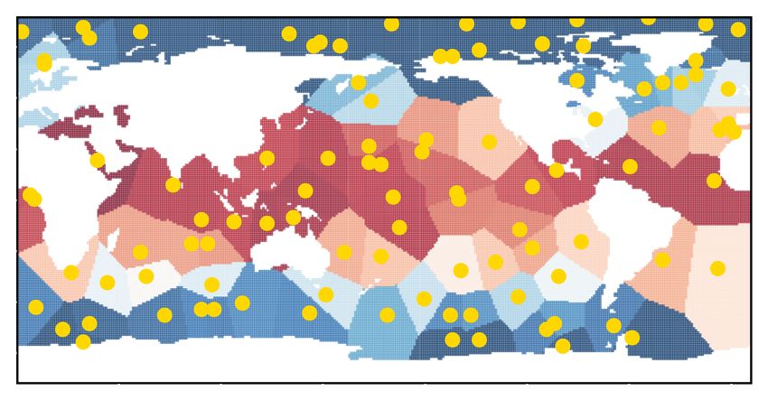
100                                150
                                                                      200                                250

                    Figure 6. Root mean squared value of streamwise velocity fluctuation in turbulent channel flow.

                          κ = 0.05                                    κ = 0.50                          κ = 1.00
Case I

                            0.290                                      0.427                              0.652
Case II

                            0.288                                      0.315                              0.372

Figure 7. Robustness of the present reconstruction technique for noisy input for the example of turbulent channel flow. Input
Voronoi tessellations (top) and reconstructed x − y sectional flow fields (bottom) are shown for Cases I and II with
κ = 0.05, 0.5, and 1.0. Reference solution is shown in figure 5.

before performing the Voronoi tessellation; and Case II: Add noise to the Voronoi tessellation input sV . For Cases I and II, the
error is assessed as

          εI = ||qqref − F (ssV (ss + κnn), s m )||2 /||qqref ||2 ,                                                           (4)
          εII = ||qqref − F (ssV + κnn, s m )||2 /||qqref ||2 ,                                                               (5)

respectively, where κ is the magnitude of the noise and n is the Gaussian distributed noise.
     The reconstructed turbulent flows for nsensor = 200 with the noisy inputs are summarized in figure 7. As shown, the input
Voronoi tessellations defined by Case II exhibit noisy features compared to those utilized by Case I since the noise for Case
II is added after the preparation of the Voronoi tessellations. The influence of noise for Case I is larger than that of Case II.
This is caused by the fact that the present CNN is trained for learning the relationship between the input Voronoi images and
high-resolution flow fields, which implies that large perturbations to the sensor measurements produce greater error to the
input images. If robustness is desired, we recommend adding noise to the sensor measurements prior to the preparation of the
Voronoi-based input images during the training process. Overall, the present reconstruction technique is found to be robust
against noise.

4 Discussion
Reconstruction of a global field variable from an arbitrary collection of sensors has been a longstanding challenge in engineering
and the sciences. In order to address this problem, we presented a data-driven global reconstruction technique comprised of
Voronoi tessellation and CNN. The present method relies on inputs of mask images holding the sensor location and Voronoi
images representing the sensor measurements. The use of Voronoi tessellation translates the input sensor data to be represented
on a uniform grid, which then enables the applications of CNNs to derive deep learning based reconstruction models. Three
examples of global flow reconstruction from local sensor measurements demonstrated the accuracy and robustness of the
current method.

                                                                                                                             7/10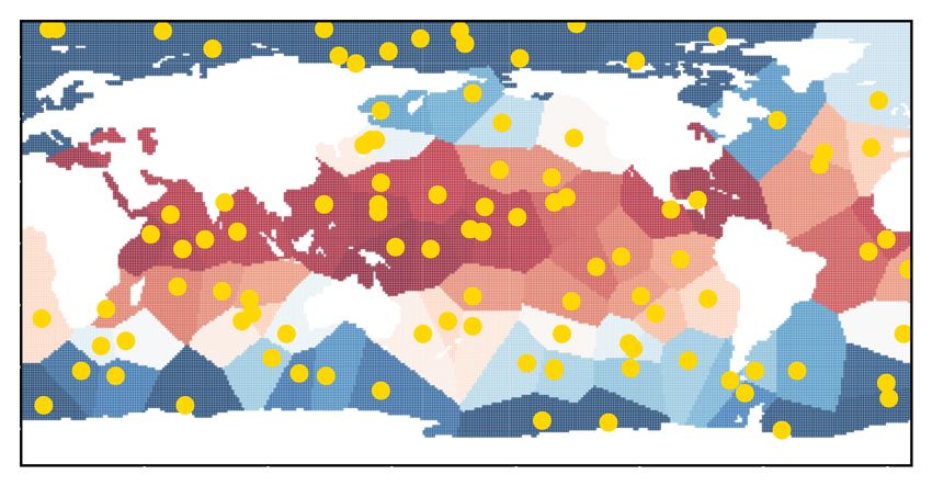
Since CNNs have a large collection of toolsets from the image processing community, the present reconstruction approach is
significant from the point of view of merging image processing with sensor data analytics. This perspective now allows engineers
and scientists to move through the wealth of local and global measurements using data-driven techniques. Furthermore, Voronoi
tessellation has the beneficial property of being able to discretize the spatial information in an adaptive manner only where
sensor arrangements change in time. This provides computational savings and an opportunity to develop spatially adaptive
techniques.
    The present approach can be extended to enforce physical constraints and properties31–34 . For example, evolutional deep
neural network35 has been able to enforce the divergence free constraint for incompressible flow. Another possible extension is
the construction of robust models with regard to physical parameters by preparing proper training data sets36–38 . To obtain
generalizable models for turbulent data sets, unsupervised learning may also be helpful38 .
    The present data-driven approach was demonstrated with a set of local sensor measurements. As this method performs
spatial field reconstruction at each time, changes in the number of sensors or motion of the sensors are easily accommodated.
Having this flexibility allows for extensions to incorporate other types of measurements, such as under-resolved satellite based
measurements or particle image velocimetry. The current formulation also opens a path to incorporate intelligent sensor
placements1 to further reduce reconstruction error and enhance the robustness with data redundancy. Moreover, the present
method can be applied to cases where output attributes are different from the input data attributes. In such a scenario, the
Voronoi-tessellation is akin to a projection operation to extend learning one step further. While we use the Voronoi CNN
solely for flow reconstruction in the present paper, high-order turbulence statistics, e.g., root-mean-squared values of velocity
fluctuations, can be extracted as well. The power and simplicity of the present approach will support scientific endeavor across
a wide range of studies for complex data structures.

Data availability
Training data used in the present study are available on Google Drive: Example 1 (two-dimensional cylinder wake): https:
//drive.google.com/drive/folders/1K7upSyHAIVtsyNAqe6P8TY1nS5WpxJ2c?usp=sharing),
Example 2 (NOAA sea surface temperature): https://drive.google.com/drive/folders/1pVW4epkeHkT2
WHZB7Dym5IURcfOP4cXu?usp=sharing), and Example 3 (turbulent channel flow): https://drive.google.c
om/drive/folders/1xIY_jIu-hNcRY-TTf4oYX1Xg4_fx8ZvD?usp=sharing).

Code availability
Sample codes for training the present models are available on GitHub (https://github.com/kfukami/Voronoi-C
NN).

References
 1. Manohar, K., Brunton, B. W., Kutz, J. N. & Brunton, S. L. Data-driven sparse sensor placement for reconstruction:
    Demonstrating the benefits of exploiting known patterns. IEEE Control. Syst. Mag. 38, 63–86 (2018).
 2. Akiyama, K. et al. First M87 event horizon telescope results. III. Data processing and calibration. The Astrophys. J. Lett.
    875, L3 (2019).
 3. Alonso, M. T., López-Dekker, P. & Mallorquí, J. J. A novel strategy for radar imaging based on compressive sensing. IEEE
    Transactions on Geosci. Remote. Sens. 48, 4285–4295 (2010).
 4. Mishra, K. V., Kruger, A. & Krajewski, W. F. Compressed sensing applied to weather radar. In 2014 IEEE Geoscience and
    Remote Sensing Symposium, 1832–1835 (IEEE, 2014).
 5. Fukami, K., Fukagata, K. & Taira, K. Assessment of supervised machine learning for fluid flows. Theor. Comp. Fluid Dyn.
    34, 497–519 (2020).
 6. Boisson, J. & Dubrulle, B. Three-dimensional magnetic field reconstruction in the VKS experiment through Galerkin
    transforms. New J. Phys. 13, 023037 (2011).
 7. Noack, B. R. & Eckelmann, H. A global stability analysis of the steady and periodic cylinder wake. J. Fluid Mech. 270,
    297–330 (1994).
 8. Adrian, R. J. & Moin, P. Stochastic estimation of organized turbulent structure: homogeneous shear flow. J. Fluid Mech.
    190, 531–559 (1988).
 9. Suzuki, T. & Hasegawa, Y. Estimation of turbulent channel flow at Reτ = 100 based on the wall measurement using a
    simple sequential approach. J. Fluid Mech. 830, 760–796 (2006).

                                                                                                                            8/10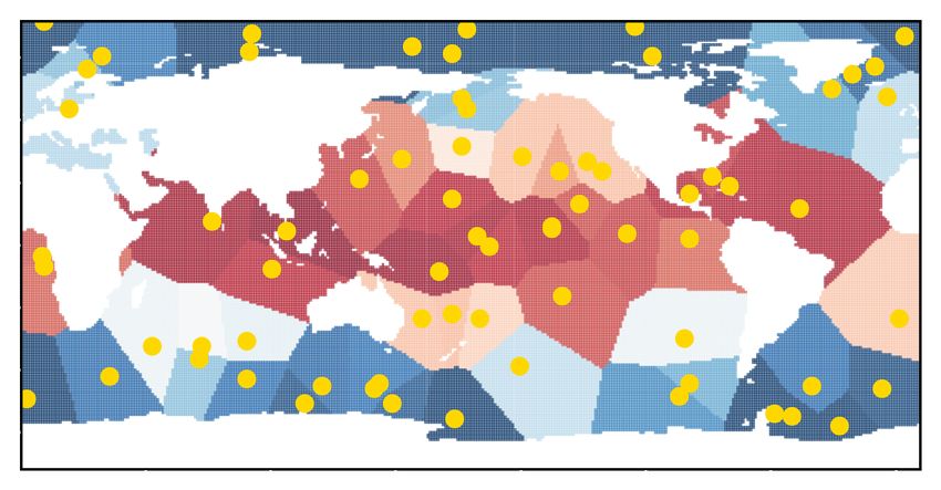
10. Bui-Thanh, T., Damodaran, M. & Willcox, K. Aerodynamic data reconstruction and inverse design using proper orthogonal
    decomposition. AIAA J. 42 (2004).
11. LeCun, Y., Bengio, Y. & Hinton, G. Deep learning. Nature 521, 436–444 (2015).
12. Brunton, S. L., Noack, B. R. & Koumoutsakos, P. Machine learning for fluid mechanics. Annu. Rev. Fluid Mech. 52,
    477–508 (2020).
13. LeCun, Y., Bottou, L., Bengio, Y. & Haffner, P. Gradient-based learning applied to document recognition. Proc. IEEE 86,
    2278–2324 (1998).
14. Fukami, K., Fukagata, K. & Taira, K. Super-resolution reconstruction of turbulent flows with machine learning. J. Fluid
    Mech. 870, 106–120 (2019).
15. Rumelhart, D. E., Hinton, G. E. & Williams, R. J. Learning representations by back-propagation errors. Nature 322,
    533—536 (1986).
16. Wu, Z. et al. A comprehensive survey on graph neural networks. IEEE Transactions on Neural Networks Learn. Syst.
    (2020).
17. Mallick, T., Balaprakash, P., Rask, E. & Macfarlane, J. Transfer learning with graph neural networks for short-term
    highway traffic forecasting. arXiv:2004.08038 (2020).
18. Chai, X. et al. Deep learning for irregularly and regularly missing data reconstruction. Sci. Rep. 10, 1–18 (2020).
19. Machicoane, N. et al. Recent developments in particle tracking diagnostics for turbulence research. In Flowing Matter,
    177–209 (Springer, Cham, 2019).
20. Voronoi, G. New applications of continuous parameters to the theory of quadratic forms. first thesis. on some properties of
    perfect positive quadratic forms. J. fur die Reine und angewandte Math. 133, 97–178 (1908).
21. Aurenhammer, F. Voronoi diagrams—a survey of a fundamental geometric data structure. ACM Comput. Surv. (CSUR) 23,
    345–405 (1991).
22. Fukami, K., Fukagata, K. & Taira, K. Machine-learning-based spatio-temporal super resolution reconstruction of turbulent
    flows. J. Fluid Mech. 909, A9 (2021).
23. Nair, V. & Hinton, G. E. Rectified linear units improve restricted boltzmann machines. Proc. Int. Conf. Mach. Learn.
    807–814 (2010).
24. Kingma, D. P. & Ba, J. Adam: A method for stochastic optimization. arXiv:1412.6980 (2014).
25. Prechelt, L. Automatic early stopping using cross validation: quantifying the criteria. Neural Netw. 11, 761–767 (1998).
26. Brunton, S. L. & Kutz, J. N. Data-driven science and engineering: Machine learning, dynamical systems, and control
    (Cambridge University Press, 2019).
27. Taira, K. & Colonius, T. The immersed boundary method: A projection approach. J. Comput. Phys. 225, 2118–2137
    (2007).
28. Colonius, T. & Taira, K. A fast immersed boundary method using a nullspace approach and multi-domain far-field boundary
    conditions. Comput. Methods Appl. Mech. Eng. 197, 2131–2146 (2008).
29. Fukagata, K., Kasagi, N. & Koumoutsakos, P. A theoretical prediction of friction drag reduction in turbulent flow by
    superhydrophobic surfaces. Phys. Fluids 18, 051703 (2006).
30. Fukami, K., Nabae, Y., Kawai, K. & Fukagata, K. Synthetic turbulent inflow generator using machine learning. Phys. Rev.
    Fluids 4, 064603 (2019).
31. Raissi, M., Perdikaris, P. & Karniadakis, G. E. Physics-informed neural networks: A deep learning framework for solving
    forward and inverse problems involving nonlinear partial differential equations. J. Comput. Phys. 378, 686–707 (2019).
32. Raissi, M., Yazdani, A. & Karniadakis, G. E. Hidden fluid mechanics: Learning velocity and pressure fields from flow
    visualizations. Science 367, 1026–1030 (2020).
33. Hasegawa, K., Fukami, K., Murata, T. & Fukagata, K. Machine-learning-based reduced-order modeling for unsteady flows
    around bluff bodies of various shapes. Theor. Comput. Fluid Dyn. 34, 367–388 (2020).
34. Lee, S. & You, D. Data-driven prediction of unsteady flow fields over a circular cylinder using deep learning. J. Fluid
    Mech. 879, 217–254 (2019).
35. Du, Y. & Zaki, T. A. Evolutional deep neural network. arXiv:2103.09959 (2021).

                                                                                                                          9/10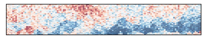
36. Morimoto, M., Fukami, K., Zhang, K. & Fukagata, K. Generalization techniques of neural networks for fluid flow
    estimation. arXiv:2011.11911 (2020).
37. Hasegawa, K., Fukami, K., Murata, T. & Fukagata, K. CNN-LSTM based reduced order modeling of two-dimensional
    unsteady flows around a circular cylinder at different Reynolds numbers. Fluid Dyn. Res. 52, 065501 (2020).
38. Kim, H., Kim, J., Won, S. & Lee, C. Unsupervised deep learning for super-resolution reconstruction of turbulence. J. Fluid
    Mech. 910, A29 (2021).

Acknowledgement
R.M. and N.R. were supported by the U.S. Department of Energy, Office of Science, Office of Advanced Scientific Computing
Research, under Contract DE-AC02-06CH11357. This research was funded in part and used resources of the Argonne
Leadership Computing Facility, which is a DOE Office of Science User Facility supported under Contract DE-AC02-06CH11357.
Ko.F. thanks support from the Japan Society for the Promotion of Science (18H03758, 21H05007). K.T. acknowledges support
from the US Air Force Office of Scientific Research (FA9550-16-1-0650 and FA9550-21-1-0178) and the US Army Research
Office (W911NF-19-1-0032).

Author contributions statement
Ka.F., R.M, and N.R. designed research; Ka.F. performed research; Ka.F. analyzed data; Ka.F. and K.T. wrote the paper; Ko.F.
and K.T. supervised. All authors reviewed the manuscript.

Declaration of interest
The authors report no conflict of interest.

                                                                                                                        10/10
You can also read