Algorithms for Nonnegative Tensor Factorization - Department of Computer Sciences
←
→
Page content transcription
If your browser does not render page correctly, please read the page content below
Algorithms for Nonnegative Tensor
          Factorization

                 Markus Flatz

 Technical Report 2013-05       November 2013

   Department of Computer Sciences

            Jakob-Haringer-Straße 2
            5020 Salzburg
            Austria
            www.cosy.sbg.ac.at

        Technical Report Series
Algorithms for Nonnegative Tensor
Factorization
Markus Flatz
Department of Computer Sciences
University of Salzburg
Salzburg, Austria
mflatz@cosy.sbg.ac.at
ABSTRACT
Nonnegative Matrix Factorization (NMF) is an efficient technique to approximate a large
matrix containing only nonnegative elements as a product of two nonnegative matrices
of significantly smaller size. The guaranteed nonnegativity of the factors is a distinctive
property that other widely used matrix factorization methods do not have.
Matrices can also be seen as second-order tensors. For some problems, it is necessary
to process tensors of third or higher order. For this purpose, NMF can be generalized to
Nonnegative Tensor Factorization (NTF). NMF and NTF are used in various application
areas, for example in document classification and multi-way data analysis.
The aim of this report is to give an overview over some algorithms to compute Nonneg-
ative Tensor Factorizations, including two multiplicative algorithm based on the Alpha-
divergence and the Beta-divergence, respectively, two Hierarchical Alternating Least
Squares algorithms and a Block Principal Pivoting algorithm utilizing matricization.
KEY WORDS
High Performance Computing, Nonnegative Tensor Factorization, Nonnegative Matrix
Factorization
1 Introduction
A characteristic property of modern society is the increasing need to process large
amounts of data. One important class of data is represented by nonnegative matri-
ces and tensors, which occur in many application areas. These are often considerably
large, which makes their processing and evaluation difficult and time-consuming.
1Nonnegative Matrix Factorization, (abbreviated as NMF or NNMF), is a technique to
approximate a nonnegative matrix as a product of two nonnegative matrices. The two
resulting matrices are usually smaller than the original matrix and therefore easier to
handle and process. In the last decade, NMF has become quite popular and has been
applied to a wide variety of practical problems.
The idea of such a factorization was published in 1994 under the name “Positive
Matrix Factorization” [21]. In 1999, an article in Nature [14] about Nonnegative Matrix
Factorization caught the attention of a wide audience. Several papers were written
about NMF since then, discussing its properties, algorithms, modifications and often also
possible applications. Some of the various areas where Nonnegative Matrix Factorization
was successfully applied are text mining [23] [24] [1], classification of documents [2] and
emails [10], clustering [28] [18], spectral data analysis [11] [22] [1], face recognition [29],
distance estimation in networks [19], the analysis of EEG data [16], separation of sound
sources [27], music transcription [25] [26], computational biology, for example molecular
pattern discovery and class comparison and prediction [3] [8] [7] and neuroscience [6].
In contrast to other methods such as singular value decomposition (SVD) or principal
component analysis (PCA), NMF has the distinguishing property that the factors are
guaranteed to be nonnegative, which allows to view the factorization as an additive
combination of features.
2 The NMF Problem
An informal description of the NMF problem is: Given a nonnegative matrix Y of size
I × T , find two nonnegative matrices A (size I × J) and X (size J × T ) such that their
product AX approximates Y. Figure 1 illustrates the NMF problem for I = 7, T = 9
and J = 3.
Y A
X
I ≈ I · J
| {z }
T
| {z } | {z }
T J
Figure 1: Illustration of the NMF problem
A matrix is called nonnegative if all its elements are ≥ 0. In practical cases, the chosen
J is usually much smaller than I and T . It should be noted that, in general, it is not
2possible to find A and X such that AX = Y. Hence, NMF is “only” an approximation,
for this reason it is sometimes called Approximative Nonnegative Matrix Factorization
or Nonnegative Matrix Approximation. This is sometimes expressed as Y = AX + E,
where E is a matrix of size I × T that represents the approximation error. Thus, AX
can be seen as a compressed representation of Y, with a rank of j or less.
Formally, NMF can be defined as [20]:
Definition (NMF). Given a nonnegative matrix Y ∈ RI×T and a positive integer J,
find nonnegative matrices A ∈ RI×J and X ∈ RJ×T that minimize the functional
1
f (A, X) = ||Y − AX||2F .
2
In [20], J < min{I, T } is explicitly required, this is not strictly necessary, but true in
almost all practical cases. For an I × T matrix M, ||M||F is the Frobenius norm of M,
defined as v
u I T
uX X
||M||F := t m2i,t
i=1 t=1
where mi,t denotes the element of M with row index i and column index t. Therefore,
f (A, X) is the square of the Euclidean distance between Y and AX with an additional
factor 12 . The problem is convex in A and in X separately, but not in both simultaneously
[9].
We note that it is also possible to use other measures to express the distance between
Y and AX, for example the Kullback-Leibler divergence [15], Csiszár’s divergences [5]
or Alpha- and Beta-divergences [6]. Different measures yield different NMF algorithms,
or at least different update steps for the algorithms.
Every column of A can be interpreted as a basis feature of size I. In total, A contains
J basis features. The multiplication of A with the nonnegative matrix X yields a
nonnegative matrix AX, where every column of AX is an additive (or non-subtractive)
combination of weighted basis features (columns of A). The famous paper on NMF in
Nature [14] uses NMF to represent faces as additive combinations of local parts such as
eyes, nose, mouth, etc. However, it was shown in [17] that NMF does not always find
such localized features.
33 The NTF Problem
Matrices are second-order tensors. For some applications, for example in multi-way data
analysis, the input data are tensors of third or higher order. Therefore, it is desirable to
generalize Nonnegative Matrix Factorization to Nonnegative Tensor Factorization.
3.1 Notation
For the formulation of the NTF problem and the algorithms, the following symbols are
used:
◦ outer product
Khatri-Rao product
~ Hadamard product
element-wise division
×n mode-n product of tensor and matrix
A −n
= A(N ) . . . A(n+1) A(n−1) . . . A(1)
3.2 Problem definition
The Nonnegative Tensor Factorization problem can be formulated as nonnegative canon-
ical decomposition / parallel factor decomposition (CANDECOMP / PARAFAC) as
follows (after [6]):
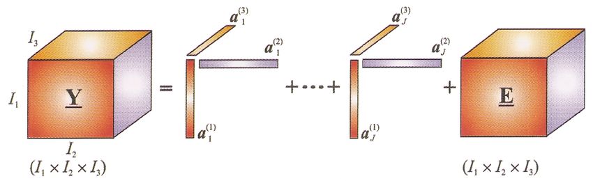
Definition (NTF). Given an N -th order tensor Y ∈ RI1 ×I2 ×...×IN and a positive integer
J, factorize Y into a set of N nonnegative component matrices
(n) (n) (n)
A(n) = [a1 , a2 , . . . , aJ ] ∈ RIn ×J , (n = 1, 2, . . . , N ) representing the common (loading)
factors, that is,
X J
(1) (2) (N )
Y = Ŷ + E = aj ◦ aj ◦ . . . ◦ aj + E =
j=1
I ×1 A(1) ×2 A(2) · · · ×N A(N ) + E = JA(1) , A(2) , . . . , A(N ) K + E
(n)
with ||aj ||2 = 1 for n = 1, 2, . . . N − 1 and j = 1, 2, . . . , J.
The tensor E is the approximation error. Figure 2 illustrates the decomposition for a
third-order tensor.
4Figure 2: The NTF model for a third-order tensor (from [6])
4 Alpha NTF
The first algorithm presented here uses multiplicative updates based on the Alpha-
divergence [6]. Multiplicative algorithms are relatively simple, but can be slower in
comparison to enhanced HALS algorithms.
Algorithm 1: Alpha NTF (from [6])
Input: Y: input data of size I1 × I2 × . . . × IN , J: number of basis components
Output: N component matrices A(n) ∈ RI+n ×J
1 begin
2 ALS or random initialization for all factors A(n) ;
(n) −1
3 Al = A(n) diag{1T A(n) } for ∀n; /* normalize to unit length */
(n)
4 A(n) = Al for ∀n 6= N ;
5 repeat
6 Ŷ = JA(1) , A(2) , . . . , A(N ) K;
7 for n = 1 to N do
.[α] .[1/α]
8 A ← A ~ Y(n) Ŷ(n)
(n) (n)
Al −n
;
(n) −1
9 Al = A(n) diag{1T A(n) } ; /* normalize to unit length */
10 if n 6= N then
(n)
11 A(n) = Al ;
12 end
13 end
14 until a stopping criterion is met;
15 end
55 Beta NTF
It is also possible to formulate a multiplicative Nonnegative Tensor Factorization algo-
rithm based on the Beta-divergence [6]:
Algorithm 2: Beta NTF (from [6])
Input: Y: input data of size I1 × I2 × . . . × IN , J: number of basis components
Output: N component matrices A(n) ∈ RI+n ×J
1 begin
2 ALS or random initialization for all factors A(n) ;
3 repeat
4 Ŷ = JA(1) , A(2) , . . . , A(N ) K;
5 for n = 1 to N doh i
.[β−1] .[β]
6 A ← A ~ Y(n) Ŷ(n)
(n) (n)
A −n
Ŷ(n) A −n
;
7 if n 6= N then
−1
8 A(n) ← A(n) diag{1T A(n) } ; /* normalize */
9 end
10 end
11 until a stopping criterion is met;
12 end
6 HALS NTF
HALS stands for Hierarchical Alternating Least Squares. The idea is to minimize a set of
local cost functions with the same global minima by approximating rank-one tensors [4].
Two algorithms are presented here, first a simple HALS algorithm (Algorithm 3) and
then another algorithm that reduces computation of the expensive Khatri-Rao products
(Algorithm 4) [6]. Both algorithms use the squared Euclidean distance, but it is also
possible to formulate HALS algorithms based on Alpha- and Beta-divergences.
6Algorithm 3: Simple HALS NTF (from [6])
Input: Y: input data of size I1 × I2 × . . . × IN , J: number of basis components
Output: N component matrices A(n) ∈ RI+n ×J
1 begin
2 ALS or random initialization for all factors A(n) ;
(n) (n) (n)
3 aj ← aj /||aj ||2 for ∀j, n = 1, 2, . . . , N − 1; /* normalize to unit
length */
4 E = Y − Ŷ = Y − J{A}K ; /* residual tensor */
5 repeat
6 for j = 1 to J do
(1) (2) (N )
7 Y(j) = E + Jaj , aj , . . . , aj K;
8 for n = 1 toh N do i
(n) (j)
9 aj ← Y(n) {aj −n } ;
+
10 if n 6= N then
(n) (n) (n)
11 aj ← aj /||aj ||2 ; /* normalize to unit length */
12 end
13 end
(1) (2) (N )
14 E = Y(j) − Jaj , aj , . . . , aj K;
15 end
16 until a stopping criterion is met;
17 end
7Algorithm 4: FAST HALS NTF (from [6])
Input: Y: input data of size I1 × I2 × . . . × IN , J: number of basis components
Output: N component matrices A(n) ∈ RI+n ×J
1 begin
2 ALS or random initialization for all factors A(n) ;
(n) (n) (n)
3 aj ← aj /||aj ||2 for ∀j, n = 1, 2, . . . , N − 1; /* normalize to unit
length */
4 T(1) = (A(1)T A(1) ) ~ · · · ~ (A(N )T A(N ) );
5 repeat
6 γ = diag(A(N )T A(N ) );
7 for n = 1 to N do
8 if n = N then
9 γ = 1;
10 end
11 T(2) = Y(n) {A −n };
12 T(3) = T(1) (A(n)T A(n) );
13 for j = 1 to J do
(n) (n) (2) (3)
14 aj ← [γj aj + tj − A(n) tj ]+ ;
15 if n 6= N then
(n) (n) (n)
16 aj ← aj /||aj ||2 ; /* normalize to unit length */
17 end
18 end
19 T(1) = T(3) ~ (A(n)T A(n) );
20 end
21 until a stopping criterion is met;
22 end
87 Block Principal Pivoting
Another way to compute a Nonnegative Tensor Factorization is called Block Principal
Pivoting, and is an active-set-like method [12] [13].
A tensor Y of size I1 × I2 × . . . × IN can be transformed into a matrix YM AT (n) in a
process called mode-n-matricization by QNlinearizing all indices except n in the following
way: YM AT (n) is a matrix of size In × k=1,k6=n Ik and the (i1 , . . . , iN )th element of Y is
mapped to the (in , L)th element of YM AT (n) where
N
X
L=1+ (ik − 1)Lk
k=1
and
k−1
Y
Lk = Ij
j=1,j6=n
For a tensor Y ∈ RI1 ×I2 ×...×IN , its approximation Ŷ = JA(1) , A(2) , . . . , A(N ) K can be
written as, for any n ∈ 1, . . . , N
T
YM AT (n) = A(n) × A −n
which can be utilized in the ANLS (alternating nonnegativity-constrained least squares)
framework. The following subproblems have to be solved:
T T 2
minA(n) ≥0 A −n
× A(n) − YM AT (n)
F
Algorithm 5 shows the Block Principal Pivoting algorithm that can be used to solve
this problem. Since the problem was reduced to a matrix problem, any NMF algorithm
could be used to compute the factorization, but algorithms that exploit the special
properties of the matrices are especially promising. (A −n is typically long and thin,
T
while A(n) is typically flat and wide.) In the formulation of the Block Principal
Pivoting algorithm below, xFl and yGl represent the subset of the lth column of X and
Y indexed by Fl and Gl , respectively.
9Algorithm 5: Block principal pivoting (from [13])
Input: V ∈ RP ×Q , W ∈ RP ×L
Output: X(∈ RQ×L = arg(minX≥0 ||VX − W||2F ))
1 begin
2 Compute VT V and VT W;
3 Initialize Fl = ∅ and Gl = {1, . . . , q} for all l ∈ 1, . . . , L;
4 X=0;
5 Y = −VT W;
6 α(∈ Rr ) = 3;
7 β(∈ Rr ) = (q + 1);
8 Compute all xFl using column grouping from VFT l VFl xFl = VFT l wl ;
9 Compute all yGl = VGTl (VFl xFl − wl );
/* (xFl , yGl ) is feasible iff xFl ≥ 0 and yGl ≥ 0 */
10 while any (xFl , yGl ) is infeasible do
11 Find the indices of columns in which the solution is infeasible:
I = {j : (xFl , yGl ) is infeasible};
12 forall the l ∈ I do
13 Hl = {q ∈ Fl : xq < 0} ∪ {q ∈ Gl : yq < 0};
14 end
15 forall the l ∈ I with |Hl | < βl do
16 βl = |Hl |;
17 αl = 3;
18 Ĥl = Hl ;
19 end
20 forall the l ∈ I with |Hl | ≥ βl and αl ≥ 1 do
21 αl = αl − 1;
22 Ĥl = Hl ;
23 end
24 forall the l ∈ I with |Hl | ≥ βl and αl = 0 do
25 Ĥl = {q : q = max{q ∈ Hl }};
26 end
27 forall the l ∈ I do
28 Fl = (Fl − Ĥl ) ∪ (Ĥl ∩ Gl );
29 Gl = (Gl − Ĥl ) ∪ (Ĥl ∩ Fl );
30 Compute xFl using column grouping from VFT l VFl xFl = VFT l wl ;
31 yGl = VGTl (VFl xFl − wl );
32 end
33 end
34 end
108 Conclusion
In this report, the Nonnegative Tensor Factorization problem was defined and five al-
gorithms to compute this factorization were presented. For future work, it would be
especially interesting to parallelize some of these algorithms to allow the processing of
large problems which arise in real-world applications on highly parallel modern comput-
ing systems.
References
[1] Michael W. Berry, Murray Browne, Amy N. Langville, V. Paul Pauca, and Robert J.
Plemmons. Algorithms and applications for approximate nonnegative matrix fac-
torization. Computational Statistics and Data Analysis, 52(1):155 – 173, 2007.
[2] Michael W. Berry, Nicolas Gillis, and François Glineur. Document classification
using nonnegative matrix factorization and underapproximation. In International
Symposium on Circuits and Systems (ISCAS), pages 2782–2785. IEEE, 2009.
[3] Jean-Philippe Brunet, Pablo Tamayo, Todd R. Golub, and Jill P. Mesirov. Meta-
genes and molecular pattern discovery using matrix factorization. Proceedings of
the National Academy of Sciences of the United States of America, 101(12):4164,
2004.
[4] Andrzej Cichocki, Anh Huy Phan, and Cesar Caiafa. Flexible HALS Algorithms
for Sparse Non-negative Matrix/Tensor Factorization. In Proceedings of 2008 IEEE
International Workshop on Machine Learning for Signal Processing, pages 73–78,
2008.
[5] Andrzej Cichocki, Rafal Zdunek, and Shun-ichi Amari. Csiszár’s divergences for
non-negative matrix factorization: Family of new algorithms. In Independent Com-
ponent Analysis and Blind Signal Separation, volume 3889 of Lecture Notes in Com-
puter Science, pages 32–39. Springer Berlin / Heidelberg, 2006.
[6] Andrzej Cichocki, Rafal Zdunek, Anh Huy Phan, and Shun-Ichi Amari. Nonnega-
tive Matrix and Tensor Factorizations: Applications to Exploratory Multi-way Data
Analysis and Blind Source Separation. John Wiley & Sons, Ltd, 2009.
[7] Karthik Devarajan. Nonnegative matrix factorization: an analytical and inter-
pretive tool in computational biology. PLoS computational biology, 4(7):e1000029,
2008.
[8] Yuan Gao and George Church. Improving molecular cancer class discovery through
sparse non-negative matrix factorization. Bioinformatics, 21(21):3970–3975, 2005.
[9] Patrik O. Hoyer. Non-negative matrix factorization with sparseness constraints.
Journal of Machine Learning Research, 5:1457–1469, 2004.
11[10] Andreas Janecek and Wilfried Gansterer. E-mail classification based on non-
negative matrix factorization. In Text Mining 2009, 2009.
[11] Arto Kaarna. Non-negative matrix factorization features from spectral signatures
of AVIRIS images. In International Conference on Geoscience and Remote Sensing
Symposium (IGARSS), pages 549–552. IEEE, 2006.
[12] Jingu Kim and Haesun Park. Fast Nonnegative Tensor Factorization with an Active-
Set-Like Method. In Michael W. Berry, Kyle A. Gallivan, Efstratios Gallopoulos,
Ananth Grama, Bernard Philippe, Yousef Saad, and Faisal Saied, editors, High-
Performance Scientific Computing – Algorithms and Applications, pages 311–326.
Springer, 2012.
[13] Jingu Kim and Haesun Park. Fast Nonnegative Tensor Factorization with an Active-
Set-Like Method. In Michael W. Berry, Kyle A. Gallivan, Efstratios Gallopoulos,
Ananth Grama, Bernard Philippe, Yousef Saad, and Faisal Saied, editors, High-
Performance Scientific Computing: Algorithms and Applications, pages 311–326.
Springer London, 2012.
[14] Daniel D. Lee and H. Sebastian Seung. Learning the parts of objects by non-negative
matrix factorization. Nature, 401:788–791, 1999.
[15] Daniel D. Lee and H. Sebastian Seung. Algorithms for Non-negative Matrix Factor-
ization. Advances in Neural Information Processing Systems (NIPS), 13:556–562,
2001.
[16] Hyekyoung Lee, Andrzej Cichocki, and Seungjin Choi. Nonnegative matrix fac-
torization for motor imagery EEG classification. In Artificial Neural Networks –
ICANN 2006, volume 4132 of Lecture Notes in Computer Science, pages 250–259.
Springer Berlin / Heidelberg, 2006.
[17] Stan Z. Li, XinWen Hou, HongJiang Zhang, and QianSheng Cheng. Learning
spatially localized, parts-based representation. In Proceedings of the 2001 IEEE
Computer Society Conference on Computer Vision and Pattern Recognition (CVPR
2001), volume 1, pages 207–212. IEEE, 2001.
[18] Tao Li and Chris Ding. The relationships among various nonnegative matrix factor-
ization methods for clustering. In Sixth International Conference on Data Mining
(ICDM’06), pages 362–371. IEEE, 2006.
[19] Yun Mao, Lawrence K. Saul, and Jonathan M. Smith. IDES: An Internet Dis-
tance Estimation Service for Large Networks. IEEE Journal on Selected Areas in
Communications (JSAC), 24(12), 2006.
[20] Gabriel Okša, Martin Bečka, and Marián Vajteršic. Nonnegative Matrix Factor-
ization: Algorithms and Parallelization. Technical Report 2010-05, University of
Salzburg, Department of Computer Sciences, 2010.
12[21] Pentti Paatero and Unto Tapper. Positive matrix factorization: A non-negative fac-
tor model with optimal utilization of error estimates of data values. Environmetrics,
5:111–126, 1994.
[22] V. Paul Pauca, J. Piper, and Robert J. Plemmons. Nonnegative matrix factorization
for spectral data analysis. Linear Algebra and its Applications, 416(1):29 – 47, 2006.
[23] V. Paul Pauca, Farial Shahnaz, Michael W. Berry, and Robert J. Plemmons. Text
mining using nonnegative matrix factorizations. In Proceedings of the Fourth SIAM
International Conference on Data Mining, pages 452–456, 2004.
[24] Farial Shahnaz, Michael W. Berry, V. Paul Pauca, and Robert J. Plemmons. Doc-
ument clustering using nonnegative matrix factorization. Information Processing
and Management, 42(2):373–386, 2006.
[25] Paris Smaragdis and Judith C. Brown. Non-negative matrix factorization for poly-
phonic music transcription. In Workshop on Applications of Signal Processing to
Audio and Acoustics, pages 177–180. IEEE, 2003.
[26] Emmanuel Vincent, Nancy Berlin, and Roland Badeau. Harmonic and inharmonic
nonnegative matrix factorization for polyphonic pitch transcription. In Interna-
tional Conference on Acoustics, Speech and Signal Processing (ICASSP), pages
109–112. IEEE, 2008.
[27] Tuomas Virtanen. Monaural sound source separation by nonnegative matrix fac-
torization with temporal continuity and sparseness criteria. Transactions on Audio,
Speech, and Language Processing, 15(3):1066–1074, 2007.
[28] Wei Xu, Xin Liu, and Yihong Gong. Document clustering based on non-negative
matrix factorization. In Proceedings of the 26th annual international ACM SIGIR
conference on research and development in information retrieval, pages 267–273.
ACM, 2003.
[29] Stefanos Zafeiriou, Anastasios Tefas, Ioan Buciu, and Ioannis Pitas. Exploiting
discriminant information in nonnegative matrix factorization with application to
frontal face verification. Transactions on Neural Networks, 17(3):683–695, 2006.
13You can also read