OLS and GWR LUR models of wildfire smoke using remote sensing and spatiotemporal data in Alberta
←
→
Page content transcription
If your browser does not render page correctly, please read the page content below
Spatial Knowledge and Information Canada, 2019, 7(2), 3

OLS and GWR LUR models of wildfire
smoke using remote sensing and
spatiotemporal data in Alberta
MOJGAN MIRZAEI                      STEFANIA B ERTAZZON           ISABELLE COULOIGNER
Department of Geography,            Department of Geography,      Department of Geography,
University of Calgary               University of Calgary;        University of Calgary
mojgan.mirzaei@ucalgary.ca          Department SAGAS,             icouloig@ucalgary.ca
                                    University of Florence
                                    bertazzs@ucalgary.ca

                                                   populations. Among these pollutants, fine
ABSTRACT                                           particles are the most harmful (WHO 2000)
                                                   During the summer of 2017, Alberta
Wildfire smoke from forest fire is a major         experienced a severe smoke episode
source of air pollution in Canadian cities.        associated with different wildfires. In mid-
Wildfire smoke includes different types of         August, smoke from wildfires in British
gases and particles that adversely affect          Columbia, Montana, Idaho and Washington
human health. Particulate Matter (PM), as          State has drifted over parts of Alberta,
the predominant pollutant in wildfire              making the air quality (AQ) so poor that it
smoke, poses the greatest risk to human            made the headlines (e.g. CBC 2017).
health. Accurate investigation of wildfire-        AQ ground stations provide the most
related PM2.5 is critical to understand            accurate data on PM2.5 concentration near
health-related    effects. This    research        the ground. However, due to their high
investigated PM2.5 concentration of wildfire       operational cost, they have sparse
smoke drifting over parts of Alberta in            distribution and limited spatial coverage,
August 2017 from British Columbia,                 especially in remote rural area.
Montana, Idaho, and as far away as                 Land Use Regression (LUR) models and
Washington State. We developed OLS and             satellite observation based models can
GWR land use regression models, which              address these limitations. A variety of
integrate the use of MODIS Aerosol Optical         studies have used LUR and remote sensing
Depth data and temporal indicators to              based     models     to    estimate   PM2.5
model PM2.5 concentration. The results             concentration (Van Donkelaar et al. 2006;
provide estimates of PM2.5 at finer spatial        Liu et al. 2007; Van Donkelaar et al. 2015;
resolution than ground-based records; these        Li et al. 2016); however, few studies
estimates could aid epidemiological studies        reported smoke-based PM2.5 estimation
to assess the health effects of wildfire           during fire periods (Mirzaei et al. 2018;
smoke.                                             Hodzic et al. 2007).
                                                   Spatial data tend to exhibit spatial non-
   1. Introduction                                 stationarity, defined as inconstant spatial
Intensity and frequency of wildfire events         variability (Anselin 1988). This spatial
have increased in recent decades and is            property can lead to spatial instability of
likely to be aggravated by climate change. In      regression coefficients (Fotheringham et al.
the past decade, wildfires have come to the        1998). Spatial non-stationarity can be
attention of public health and ecosystem           addressed by geographically weighted
studies (Youssouf et al. 2014). Wildfire PM        regression (GWR) (Fotheringham et al.
and gaseous products can lead to acute and         1998).
long term health impacts on exposed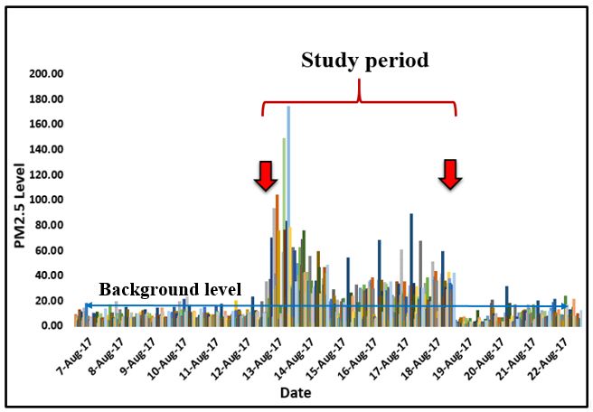
The present study aimed to assess the 2.2.1 Temporal and spatial predictors
performance of local GWR LUR to estimate Temporal variables were wind speed,
PM2.5 concentration associated with temperature, and humidity collected hourly
wildfire in Alberta in August 2017 compared at each monitoring station and averaged
to the linear method. over the study period.
Spatial variables were industrial PM2.5
2. Methods and Data emission sources, road length, vegetation
2.1 Study area and ground-based index, elevation, and distance from sources
PM2.5 measurements of fires. Industrial sources and road length
The study area (Figure 1) includes all were calculated over circular buffers of 5
Alberta Airshed Zones (AAZ). Twenty-four- and 10 km for industrial and 1 km for the
hour PM2.5 concentration were collected at road around each station. The Alberta road
49 continuous AQ stations located in AAZ 1 network was acquired from the National
over an extended period (Aug 7 to 22), Road Network (NRN 2015), and industrial
centered on the fire event (August 13-18) emission sources from the National
and including 6 days before and 4 days after Pollutant Release Inventory (NPRI 2016).
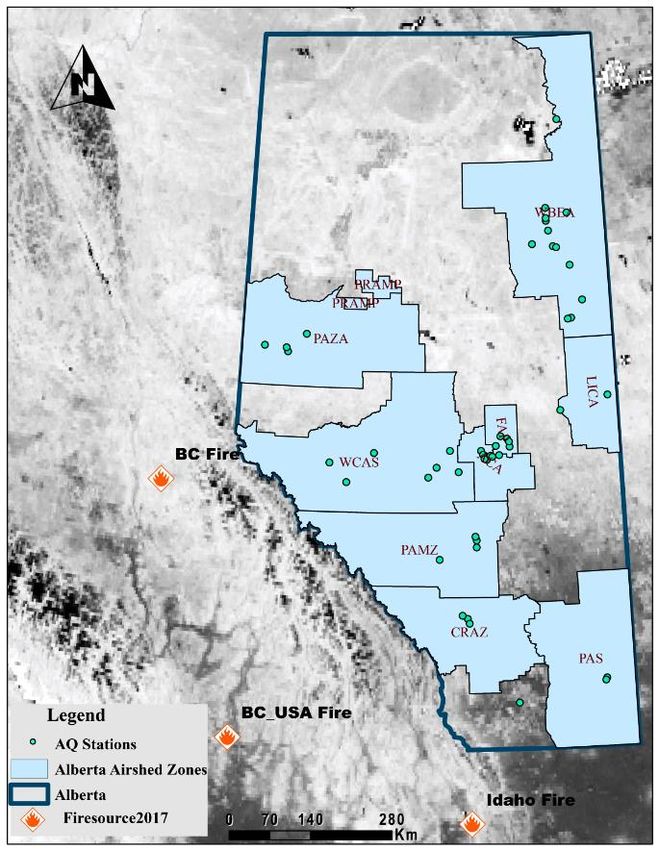
the event. Daily PM2.5 concentrations Normalized Difference Vegetation Index
(Figure 2) were averaged for the fire event (NDVI) images (MOD13C2) were used as an
period in each station. indicator of vegetation cover. The 3 km
spatial resolution (SR) images for August
2017 were collected from the NASA
Giovanni website (Acker & Leptoukh 2007).
Elevation data were acquired from DMTI
Spatial (DMTI 2010).
As the 2017 wildfire originated in different
locations, three points were considered as
sources of fire: one in BC, one in
southwestern Alberta on the Canada-USA
border, and one in Idaho (USA) (Figure 1).
The Euclidean distance between each AQ
station in the study area and each source of
the fire was calculated and included in the
model as a predictor.
The predictor variables pertaining to each
AQ station location are presented in Table 1.
2.3 AOD images
Daily AOD images at 10x10 km SR, derived
from MODIS terra collection data (NEO
2017) for the period of interest, were used as
the AOD predictor. Further, averaged AOD
product of MODIS at 1 degree, about 100
km, SR were collected from the NASA
Figure 1. Distribution of the 49 Air Quality
Giovanni website (Acker & Leptoukh 2007).
monitoring stations within the study
area. They were used to fill some of the gaps in
the 10x10 AOD images: 5x5 mean filter was
2.2 Predictors applied, wherever possible, to calculate the
The LUR model relied on the following missing values of the finer resolution images
predictor categories. from their surrounding pixels; in areas
where no surrounding pixels existed, the
1http://airdata.alberta.ca/RelatedLinks.asp
coarser resolution images were used to
xLUR modelling of wildfire smoke in Alberta 3
simply fill gaps of the finer resolution image concentration is under background level (20
with its values. µg/m3) almost for all stations before and
2.4 Prediction Models after the smoke event. It can also be seen
Traditional LUR models are described by that the daily averaged PM2.5 concentration
standard regression equations (Eq.1), where raised dramatically on August 13 and
the response variable yi, i.e. observed PM2.5 remained elevated until August 18.
concentration at location i is expressed as a Descriptive statistics of PM2.5 concentration
function of k land use predictors, i.e., xi1 over the study period are presented in Table
through xik, such as those detailed in Table 1. 1.
The 0 through k coefficients are estimated
using ordinary least squares (OLS).
∑ ( )
Since global Moran’s I spatial statistical test
(Florax et al. 2003; Getis and Aldstadt
2004) of the PM2.5 concentration (Table 1)
indicated that there was significant spatial
autocorrelation, showing a likelihood of a
clustered pattern, GWR was applied.
GWR applies a spatial weighting function on
the spatial coordinates of each data point, Figure 2. Daily variability of PM2.5 concentration at the 49
stations located in the study area.
i.e. (ui, vi), to subdivide the study area into
local neighbourhoods, where local Table 1. Descriptive statistics of response
regressions are calculated (Eq. 2). (PM2.5) and predictor variables
Consequently, GWR produces n local Response
regressions, each of them linear, and each Min Max Moran’I P(I)
Variable
one over a neighbourhood defined by the PM2.5 9.85 57.9 0.6 0.00
kernel function. A fixed bandwidth with a Predictors Name/ Description
Unit/
Range
Gaussian kernel was selected. The Resolution
Merged Aerosol
bandwidth was determined automatically by AOD
Optical Depth
10x10 km 0.57
minimizing a leave-one-out cross-validation NDVI Vegetation Index 3x3 km 0.59
(CV) score (Fortheringham et al. 2002).
TEMP Temperature Celcius 20.31
( ) ∑ ( ) ( ) RH Relative humidity Percentage 75.30
km/hr at 10
WSP Wind speed 17.62
Forward stepwise multiple linear regression m height
(SMLR) was employed as a variable Ind_5km/
Industrial points
Points in
selection procedure to identify the around each station 29 / 41
10km buffer
within 5 and 10 km
significant predictors in the regression Length in
model. Road 1km
Road length around
buffer 46,711
each station
LUR models were calculated in R (R Core (meter)
Team 2018) using mainly the ‘spdep’ ELV Elevation meter 1171.28
(Bivand & Piras 2015; Bivand et al. 2013), Distance from fire
BC-Dis kilometre 628,725
‘GWmodel’ (Gollini et al. 2013), ‘car’ (Fox & in BC
Weisberg 2011), and ‘lmtest’ packages Idaho-Dis
Distance from fire
kilometre 997,808
in Idaho
(Zeileis & Hothorn 2002).
Distance from fire
BC-US-dis kilometre 749,683
3. Results and Discussion in BC_USA border
Figure 2 shows the daily variability of PM 2.5
concentration recorded at the 49 AQ The variables identified by SMLR included
stations. The figure shows that PM2.5 AOD, wind speed, temperature, elevation,4 LUR modelling of wildfire smoke in Alberta
and BC-distance. AOD, followed by wind PM. Similar results were obtained by our
speed and temperature, were the three most recent study of LUR models before, during,
significant variables in both OLS and GWR and after wildfire events (Mirzaei et al.
models. 2018).
Table 2 and Table 3 present the statistical Table 3: GWR results
results of OLS and GWR models
respectively. The OLS LUR yielded a Coef Coef t-Value t-Value
relatively high goodness-of-fit, with R2 of median range mean range
0.74 and adjusted R2 of 0.71. However, the Intercept 37.4 25.5 3.98 2.2
model performance was improved AOD 16.4 42.6 1.72 4.79
substantially by the use of GWR, with WSP -1.14 1.28 -3.6 0.05
higher R2, and lower AIC and RSS values TEMP 0.67 0.48 2.8 2.91
compared to the OLS model. ELV 9.0E-03 8.6E-03 1.63 1.17
BC-Dis -4.4E-05 4.8E-05 -5.5 3.78
2 2
Table 2: OLS results R 0.84 Adj.R 0.77
AIC 288 RSS 830
Coef Std.Error P-Value LMerr Res 1.92 Res Moran’s I -0.11
Intercept 34.4 8.52 0.00
AOD 14.9 7.33 0.04 Observed versus GWR predicted PM2.5
WSP -1.23 0.28 0.00 concentration, as well as OLS and GWR
TEMP 0.67 0.23 0.00 residuals are shown in Fig. 3.
ELV 9.8E-03 5.3E-03 0.07 The observed PM2.5 concentration is higher
BC-Dis -3.8E-05 7.1E-06 0.00 in the western parts of Alberta mainly due
R
2
0.74 Adj.R
2
0.71 to the longer distance to the fire(s) of
AIC 313 RSS 1306 interest. The GWR fitted concentration
LMerr Res 0.005 Res Moran’s I -0.006 follows this pattern through its association
with the selection of distance to BC wildfire
Roads and industries are known as two among all three sources of fire.
important sources of PM2.5 in cities; It can be seen in the residuals maps that not
however, these two variables were not only did the GWR model performed better
significant in these models and were than the OLS model, but also that this
removed on the SLRM variable selection difference is greater for lower PM2.5
procedure. This result indicates that the concentration (shown in grey), relative to
presence/absence of wildfire smoke affects higher concentration. Over- and under-
the model’s predictors, as meteorological estimates do not present any spatial pattern
variables dominate the model, extruding but demonstrate that more work needs to be
those variables normally associated with done for a more accurate model.LUR modelling of wildfire smoke in Alberta 5
Figure 3 Observed and GWR predicted PM2.5 concentration, as well as OLS LUR and GWR LUR residuals
(orange corresponds to underfitted values and blue to overfitted ones)
due to wildfire smoke using OLS and GWR
4. Conclusion land use regression that integrated MODIS
Due to wildfire events from BC and the AOD, meteorological data, and spatial
USA, some parts of Alberta experienced a variables. The OLS results indicated that the
high level of smoke and PM2.5 global model performed relatively well;
concentration in August 2017. however, the GWR LUR has achieved a
In the present study, we modelled the better model performance, as shown by
spatial distribution of PM2.5 concentration higher R2 and lower AIC and RSS.6 LUR modelling of wildfire smoke in Alberta
Overall, we have demonstrated the potential DMTI, 2010. The Gold Standard Canada’s Most
of integrating satellite AOD data with spatial Complete and Accurate Mapping Data.
and temporal variables to accurately predict DMTI Spatial. Available at:
PM2.5 concentration during wildfire smoke https://www.dmtispatial.com/ [Accessed
events. Building on these promising results, August 22, 2018].
our models can be further improved by Fotheringham, A.S., Charlton, M.E. &
using more spatiotemporal variables and Brunsdon, C., 1998. Geographically
better methodology to fill AOD images’ Weighted Regression: A Natural Evolution
gaps, so that we can develop daily models of of the Expansion Method for Spatial Data
the PM2.5 plume. Analysis. Environment and Planning A:
Economy and Space, 30(11), pp.1905–
1927.
Acknowledgment Fotheringham, A. S., Brunsdon, C., & Charlton,
Mojgan Mirzaei wishes to thank “Eyes High M. (2002). Geographically Weighted
Doctoral Recruitment Scholarship” for Regression: The Analysis of Spatially
supporting her doctoral work. Stefania Varying Relationships. Chichester: Wiley
Bertazzon wishes to thank the Canadian Fox, J. & Weisberg, S., 2011. An R Companion
Institutes for Health Research (CIHR) Institute to Applied Regression, Second Edition,
for Population and Public Health for funding the Sage Publications. Available at:
research on air pollution and public health. We https://socialsciences.mcmaster.ca/jfox/Bo
are grateful to our colleagues and members of oks/Companion-2E/index.html.
the Geography of Health research group of the Florax RJGM, Folmer H, Rey SJ, 2003.
O’Brien Institute for Population Health for their Specification searches in spatial
advice and insightful discussions. econometrics: the relevance of Hendry’s
References methodology. Reg Sci Urban Econ, 33(5),
Acker, J.G. & Leptoukh, G., 2007. Online 557–79.
Analysis Enhances Use of NASA Earth Getis A. and Aldstadt J., 2004. Constructing the
Science Data. Eos, Transactions American spatial weights matrix using a local
Geophysical Union, 88(2), p.14. Available statistic. Geogr Anal, 40, 297–309
at: Gollini, I. et al., 2013. GWmodel: an R Package
http://doi.wiley.com/10.1029/2007EO0200 for Exploring Spatial Heterogeneity using
03. Geographically Weighted Models.
Anselin, L., 1988. Spatial econometrics: Available at:
methods and models Springer., Kluwer, http://arxiv.org/abs/1306.0413.
New York. Available at: Hodzic, A. et al., 2007. Wildfire particulate
https://www.springer.com/gp/book/978902 matter in Europe during summer 2003:
4737352. Meso-scale modeling of smoke emissions,
Bivand R. et al., 2013. Applied Spatial Data transport and radiative effects.
Analysis with R Springer, ed., New York. Atmospheric Chemistry and Physics, 7(15),
Bivand, R. & Piras, G., 2015. Comparing pp.4043–4064.
Implementations of Estimation Methods Li, S., Joseph, E. & Min, Q., 2016. Remote
for Spatial Econometrics. Journal of sensing of ground-level PM2.5 combining
Statistical Software, 63(18). Available at: AOD and backscattering profile. Remote
http://www.jstatsoft.org/v63/i18/. Sensing of Environment, 183, pp.120–128.
CBC, 2017. “High risk” air quality warning Available at:
issued for Calgary as B.C. wildfire smoke http://dx.doi.org/10.1016/j.rse.2016.05.025
returns. CBC News. Available at: .
https://www.cbc.ca/news/canada/calgary/c Liu, Y. et al., 2007. Using aerosol optical
algary-air-quality-index-health-aqhi-bc- thickness to predict ground-level
forest-fires-alberta-smoky-skies-august-31- PM2.5concentrations in the St. Louis area:
1.4269864. A comparison between MISR and MODIS.LUR modelling of wildfire smoke in Alberta 7
Remote Sensing of Environment, 107(1–2), Zeileis, A. & Hothorn, T., 2002. Diagnostic
pp.33–44. Checking in Regression Relationships. R
Mirzaei, M., Bertazzon, S. & Couloigner, I., News, 2(3), pp.7–10. Available at:
2018. Modeling Wildfire Smoke Pollution https://cran.r-project.org/doc/Rnews/.
by Integrating Land Use Regression and
Remote Sensing Data: Regional Multi-
Temporal Estimates for Public Health and
Exposure Models. Atmosphere, 9(9),
p.335. Available at:
http://www.mdpi.com/2073-4433/9/9/335.
NEO, 2017. NEO, Nasa Earth Observations.
NASA. Available at:
https://neo.sci.gsfc.nasa.gov/view.php?data
setId=MODAL2_D_AER_OD&date=2018
-08-01.
NPRI, 2016. National Pollutant Release
Inventory. Environment and Climate
Change Canada. Available at:
http://www.ec.gc.ca/inrp-
npri/default.asp?lang%BCEn&;n%BC4A5
77BB9-1 [Accessed August 22, 2018].
NRN, 2015. National Road Network - NRN.
Natural Resources Canada. Available at:
https://open.canada.ca/data/en/dataset/3d28
2116-e556-400c-9306-ca1a3cada77f.
Van Donkelaar, A. et al., 2015. High-Resolution
Satellite-Derived PM 2.5 from Optimal
Estimation and Geographically Weighted
Regression over North America.
Environmental Science & Technology,
49(17), pp.10482–10491. Available at:
http://pubs.acs.org/doi/10.1021/acs.est.5b0
2076.
Van Donkelaar, A., Martin, R. V. & Park, R.J.,
2006. Estimating ground-level PM2.5
using aerosol optical depth determined
from satellite remote sensing. Journal of
Geophysical Research: Atmospheres,
111(21), pp.1–10.
WHO, 2000. Air quality guidelines for Europe.
Environmental Science and Pollution
Research, 3(1), pp.23–23. Available at:
http://link.springer.com/10.1007/BF02986
808%5Cnhttp://www.springerlink.com/ind
ex/10.1007/BF02986808.
Youssouf, H. et al., 2014. Quantifying wildfires
exposure for investigating health-related
effects. Atmospheric Environment, 97,
pp.239–251. Available at:
http://dx.doi.org/10.1016/j.atmosenv.2014.
07.041.You can also read