An End-to-End learnable Flow Regularized Model for Brain Tumor Segmentation
←
→
Page content transcription
If your browser does not render page correctly, please read the page content below
An End-to-End learnable Flow Regularized
                                              Model for Brain Tumor Segmentation

                                                         Yan Shen, Zhanghexuan Ji and Mingchen Gao

                                              Department of Computer Science and Engineering, University at Buffalo,
                                                        The State University of New York, Buffalo, USA

                                              Abstract. Many segmentation tasks for biomedical images can be mod-
                                              eled as the minimization of an energy function and solved by a class of
arXiv:2109.00622v1 [cs.CV] 1 Sep 2021

                                              max-flow and min-cut optimization algorithms. However, the segmen-
                                              tation accuracy is sensitive to the contrasting of semantic features of
                                              different segmenting objects, as the traditional energy function usually
                                              uses hand-crafted features in their energy functions. To address these
                                              limitations, we propose to incorporate end-to-end trainable neural net-
                                              work features into the energy functions. Our deep neural network features
                                              are extracted from the down-sampling and up-sampling layers with skip-
                                              connections of a U-net. In the inference stage, the learned features are fed
                                              into the energy functions. And the segmentations are solved in a primal-
                                              dual form by ADMM solvers. In the training stage, we train our neural
                                              networks by optimizing the energy function in the primal form with reg-
                                              ularizations on the min-cut and flow-conservation functions, which are
                                              derived from the optimal conditions in the dual form. We evaluate our
                                              methods, both qualitatively and quantitatively, in a brain tumor seg-
                                              mentation task. As the energy minimization model achieves a balance
                                              on sensitivity and smooth boundaries, we would show how our segmen-
                                              tation contours evolve actively through iterations as ensemble references
                                              for doctor diagnosis.

                                        1   Introduction

                                        Brain Tumors are fatal diseases affecting more than 25,000 new patients every
                                        year in the US. Most brain tumors are not diagnosed until symptoms appear,
                                        which would significantly reduce the expected life span of patients. Having early
                                        diagnosis and access to proper treatments is a vital factor to increase the survival
                                        rate of patients. MRI image has been very useful in differentiating sub-regions of
                                        the brain tumor. Computer-aided automatic segmentation distinguishing those
                                        sub-regions would be a substantial tool to help diagnosis.
                                            Among these automatic medical imaging algorithms, the advent of deep
                                        learning is a milestone. These multi-layer neural networks have been widely de-
                                        ployed on brain tumor segmentation systems. Chen et al. [3] uses a densely con-
                                        nected 3D-CNN to segment brain tumor hierarchically. Karimaghaloo et al. [10]
                                        proposes an adaptive CRF following the network output to further produce a
                                        smooth segmentation. Qin et al. [15] and Dey et al. [5] use attention model as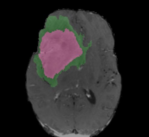
2        Y. Shen et al.

modulations on network model. Zhou et al. [18] uses transfer learning from dif-
ferent tasks. Spizer et al. [16] and Ganaye et al. [6] use spatial correspondence
among images for segmentation. Le et al. [12] proposes a level-set layer as a
recurrent neural network to iteratively minimize segmentation energy functions.
These methods combine the benefit of low inductive bias of deep neural network
with smooth segmentation boundaries.
    One fundamental difficulty with distinguishing tumor segmentation is that
their boundaries have large variations. For some extreme conditions, even expe-
rienced doctors have to vote for agreements for a final decision. Under those cir-
cumstances, a unique deterministic output of segmentation result is insufficient.
Active contour models (ACMs), which is firstly proposed by Kass et al. [11], are
widely applied in biomedical image segmentation before the era of deep learning.
ACMs treat segmentation as an energy minimization problem. They are able to
handle various topology changes naturally by providing multiple optimal solu-
tions as a level set with different thresholds. In the past two decades, quite a
number of variations of ACMs have been proposed, such as active contour with-
out edge [2], with balloon term [4]. Yuan et al. [17] proposes a flow based track
for deriving active segmentation boundaries. The evolving boundaries provide a
coarse to fine separation boundary from the background.
    In this paper, we present a trainable deep network based active contour
method. Deep neural network has tremendous advantages in providing global
statistics at semantic level. However, deep features do not preserve the bound-
ary geometry, such as topology and shapes. In our model, we explicitly use the
active contour to model the boundary and optimize its flow information. Differ-
ent from traditional active contour methods, the energy function takes neural
network trained features. The energy minimization problems are reformulated
as a max-flow/min-cut problem by introducing an auxiliary dual variable in-
dicating the flow transportation. We link the optimal segmentation conditions
with the saturated flow edges with minimal capacities. By utilizing this property,
we design a trainable objective function with extra flow regularization terms on
these saturated edges. Our work combines the benefit of deep neural network
and active contour models.
    Our contributions can be summarized as follows: (1) We present a trainable
flow regularized loss combined with neural network architecture, leveraging the
benefits of feature learning from neural networks and the advantages of regular-
izing geometry from active contour models. (2) Our results achieve comparable
results with state-of-the-art, and more importantly, show that they are flexible
to be adjusted to meet the ambiguity nature of biomedical image segmentation.

2     Methods
2.1    Image Segmentation as Energy Minimization Problem
Chan et al. [1] considered image segmentation with minimizing the following
energy functions
            Z                       Z                Z
     min       (1 − λ(x))Cs (x)dx +   λ(x)Ct (x)dx +   Cg (x)|∇λ(x)|dx (1)
    λ(x)∈{0,1}   Ω                    Ω                  Ω
Flow Regularized Model for Brain Tumor Segmentation      3

where Cs (x) is foreground pixels, Ct (x) is background pixels and Cg (x) is edge
pixels. As a naive treatment, Cs (x) and Ct (x) could use a simple thresholding
of original image, Cg (x) could use a filtered version of original image by Sobel
edge detectors.
Relation to Level Set Chan et al. [1] constructs a relationship between the
global optimum of the binary relaxed problem of λ(x) ∈ [0, 1] with the origi-
nal binary problem (1). Specifically, let λ∗ (x) be a global optimum of (1), its
thresholding λl (x) defined as
                                   (
                                     0    whenλ∗ (x) > l
                          λl (x) =                                            (2)
                                     1    whenλ∗ (x) ≤ l
is a global solution for (1) with any l ∈ [0, 1]. The function λl (x) indicates the
level set S l .

2.2     Reformulation as Max-Flow/Min-Cut Problem
The above energy minimization model for image segmentation could be trans-
formed as the well-known max-flow/min-cut [7] problems
                      Z             Z
       max     min       ps (x)dx +   λ(x)(divp(x) − ps (x) + pt (x))dx
          ps ,pt ,p λ(x)∈{0,1}    Ω               Ω
                       s.t       ps (x) ≤ Cs (x), pt (x) ≤ Ct (x), |p| ≤ Cg (x)   (3)
where ps , pt and divp are inflow, outflow and edgeflow capacity with constraints
up to the term Cs , Ct and Cg in energy minimization functions. The correlations
with flow model are shown in Fig. 1. We give a ADMM [13] solution in Algorithm
1.
  Algorithm 1: ADMM Algorithm for Segmentation Inference
   Input: Cs (x), Ct (x), Cg (x), Nt
   Output: p∗s (x), p∗t (x), p, λ∗ (x)
               1       1       1   1
 1 Initialize ps (x), pt (x), p , λ (x)
 2 for i = 1: Nt do
 3      Optimizing p by fixing other variables
         pi+1 =: arg max|p|≤Cg (x) − 2c |divp − ps + pt |2 + Ω λdivpdx
                                                             R

 4      pi+1 =:Proj [pi + α∇(divp − ps + pt )]|pi+1 (x)|≤Cg (x)
 5      Optimizing ps by fixing other variables
         pi+1 =: arg maxps ≤Cs (x) − 2c |divpp − ps + pt |2 + Ω (1 − λ)ps dx
                                                              R
           s
 6      pi+1
         s   =Proj [pis + α(divp + pt − −ps − (λ − 1)/c)]pi+1 (s)≤Cs (x)
 7      Optimizing pt by fixing other variables
         pi+1 =: arg maxpt ≤Ct (x) − 2c |divpp − ps + pt |2 + Ω λpt dx
                                                              R
           t
 8      pi+1
         t   =Proj [pit + α(−divp − pt + ps + λ/c)]pi+1 (s)≤Cs (x)
 9      Optimizing λ by fixing      other variables
         λi+1 =: arg minλ Ω λ(divp − ps + pt )dx
                             R

10      λi+1 =: λi − α(divp − ps + pt )
11    p∗s := pN
              s
                t +1
                     , p∗t := pN
                               t
                                 t +1
                                      , p∗ := pNt +1 , λ∗ := λNt +1
4      Y. Shen et al.

2.3   Optimal Conditions for Max-flow/min-cut model
The optimal condition for max-flow/min-cut model could be given by

                           λ∗ (x) = 0 =⇒ p∗s (x) = Cs (x)                                    (4)
                           λ∗ (x) = 1 =⇒ p∗t (x) = Ct (x)                                    (5)
                        |∇λ∗ (x)| =
                                  6 0 =⇒ |p| = Cg (x)                                        (6)

As it is shown in Fig. 1, an in-
tuitive explanation for the opti-
mal condition is that the incom-
                                                   Background cut
ing flow saturates at the opti-          S
mal segmentation masks of back-                                     Segmentation edge cut
ground, the outgoing flow satu-                                                  Foreground
rates at the optimal segmentation
masks of foreground and the spa-         Inflow
tial flow saturates at the segmen-        !" ($)

                                                                                            Foreground cut
tation boundaries.                                                                Outflow
                                                                                   !& ($)
                                      Background
2.4 Proposed Flow                                             Inner-flow
Regularized Training Losses                                     !' ($)

In our proposed methods, Cs (x),                                            T
Ct (x) and Cg (x) are taken from
neural network output features Fig. 1. The max-flow/min-cut model for seg-
rather than handcrafted features mentation.
in traditional methods. Specifi-
cally, our Cs (x), Ct (x) and Cg (x)
come from the parameterized outputs of a deep U-Net as shown in Fig. 2.
    Our U-Net takes the standardized input of four-modalities (T1, T2, Flair
and T1c) MRI images. Then it passes through three down-sampling blocks. Each
down-sampling block consists of a cascade of a 3 × 3 convolutional layer of stride
2 and another 3 × 3 convolutional layer of stride 1 to reduce the size of feature
map by half. The number of feature maps downward are 32, 64 ,64, 128, 128 and
256. Following the bottle-neck layers, our U-Net takes three up-sampling blocks.
Each up-sampling block consists of a cascade of a 5 × 5 deconvolutional layer
of stride 2 and another 3 × 3 convolutional layer of stride 1 to increase the size
of feature map one time. Besides the feed-forward connections, our U-Net also
consists skip connections between layers of the same horizon. Following the last
layer of the deconvolutional block, the skip-connected feature maps are passing
through the final 3 × 3 convolutional layer of stride 1 to the final layer of 9
feature maps. These 9 feature maps are divided into 3 groups. Each group takes
3 feature maps as input of Cs (x), Ct (x) and Cg (x). The three different groups
are used to segment the whole tumor area, tumor core area and enhanced tumor
core area from background hierarchically.
 Recall that the saturated min-cut condition at optimal λ∗ (x) in (4), (5), (6)
Flow Regularized Model for Brain Tumor Segmentation                                     5

                                                                                               WT/ Bg TC/ Bg    ET/ Bg

                                                                                      */ (-)
 Four channel   T1   T1c    T2   Flair
 inputs                                                                               *0 (-)

                                                                                      *+ (-)

                     32@                           Skip Connection
                                                                                                               32@

                           64@                                                                         64@
                                                   Skip Connection
                                 64@                                                               64@

                                         128@                                                  128@
                                                         Skip Connection
                                            128@              128@                   128@
          3×3 convolution, Relu            256@
                                                                              256@
          3×3 convolution, Stride 2×2,Relu
          5×5 de-convolution, Stride 2×2,Relu         Bottle-Neck Layer

Fig. 2. Our U-Net takes all four modalities MRI input and produces 9 feature maps
output into 3 groups of Cs (x) , Ct (x) and Cg (x).

and the flow conservation constraints (3), we have the followings
                            lflow = |p̂∗s − p∗s | + |p̂∗t − p∗t | + |p̂∗ − p∗ | = 0                                   (7)
where p̂∗s , p̂∗t and p̂∗ are defined as
                                       (
                                 ∗       Cs (x)               if λ∗ (x) = 0
                               p̂s =                                                                                  (8)
                                         p∗s                  if λ∗ (x) = 1
                                       (
                                         Ct (x)               if λ∗ (x) = 1
                               p̂∗t =                                                                                 (9)
                                         p∗t                  if λ∗ (x) = 0
                               (
                                   p∗                                if |∇λ∗ (x)| = 0
                         p̂∗ =                                                                                       (10)
                                   p∗ Cg (x)/|p∗ |                   if |∇λ∗ (x)| =
                                                                                  6 0

    The above equation holds as a result of joint optimal conditions of prime and
duality. At the optimal points of primal variables λ∗ saturated flows at cutting
edges equal to its maximum capacity constraints. And at the optimal points of
dual variables p∗s , p∗t and p∗ , the flow conservation function holds. By training
on lf low , we close both the primal and duality gaps at the point of ground truth
segmentation λ∗ . In our training function, we use Huber loss on lf low .
    Our whole training loss function consists of an energy minimization term and
a flow-regularized term as shown in Fig. 3.
                       Z                    Z                   Z
Ltrain = Lδ (lflow ) −     λ∗ (x)Cs (x)dx +    λ∗ (x)Ct (x)dx +    Cg (x)|∇λ∗ (x)|dx
            | {z }       Ω                   Ω                   Ω
             flow loss |                             {z                            }
                                                                      energy loss
                                                                                                                     (11)
6        Y. Shen et al.

Fig. 3. Our loss term includes two terms of energy loss and flow loss. The energy loss is
in the same form as energy minimization function. The flow loss is in the form of primal-
duality gaps between flows ps , pt and p and segmentation feature maps Cg (x), Ct (x)
and Cs (x). We enforce the constraints of optimal condition in the form of background
mask on inflow Cs (x) and ps , foreground mask in outflow Ct (x) and pt and boundary
masks in edgeflow Cg (x) and p.

Our U-net is trained end-to-end by Algorithm 2.
 Algorithm 2: U-Net Training Algorithm
   Input: λ∗ (x), Image I , α, Nt
   Output: network parameters φ
                  1
 1 Initialize φ
 2 for i = 1: Nt do
 3     Feeding forward I
 4     Cs (x), Ct (x), Cg (x) := fφi (I)
 5     Running segmentation inference algorithm
 6     p∗s (x), p∗t (x), p∗g (x) := Infer(Cs (x), Ct (x), Cg (x))
 7     Getting flow regularization loss from segmentation label
 8     Lδ (p̂∗s + −p̂∗t − div p̂∗ )
 9     Getting      energy minimization      loss from segmentation    label
                ∗                           ∗                          ∗
       R                            R                     R
10
         Ω
            −λ    (x)C  s (x)dx   +   Ω
                                        λ(x)  C t (x)dx +   Ω
                                                              Cg (x)|∇λ  (x)|dx
11     Updating φ from loss gradient
12     φi+1 := φi − α∇(Ltrain )
13   φ := φNt +1

3     Experiments

Experiment Settings We evaluate our proposed methods in BRATS2018 [14]
dataset and compare it with other state-of-the-art methods. We randomly split
the dataset of 262 glioblastoma scans of 199 lower grade glioma scans into train-
ing (80%) and testing (20%). We evaluate our methods following the BRATS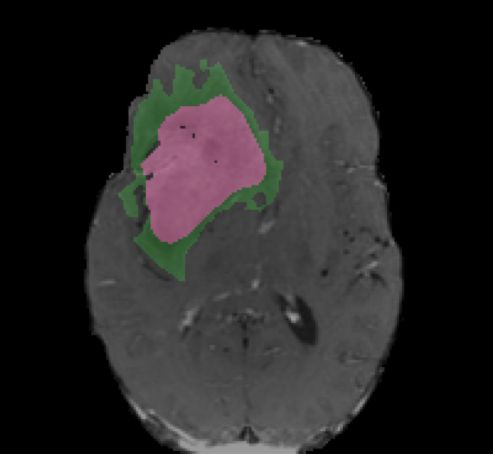
Flow Regularized Model for Brain Tumor Segmentation                   7

challenge suggested evaluation metrics of Dice, Sensitivity (Sens) and Specificity
(Spec) and Hausdorff. And we report our segmentation scores in three categories
of whole tumor area (WT), tumor core (TC) and enhance tumor core (EC).

Table 1. Segmentation results in the measurements of Dice score, Sensitivity and
Specificity.

                       Dice Score                   Sensitivity                  Specificity
               WT         TC        EC      WT         TC         EC      WT        TC         EC
Deep Medic [8] 0.896      0.754     0.718   0.903      0.73        0.73   N/A       N/A        N/A
 DMRes [9] 0.896          0.763     0.724   0.922      0.754      0.763   N/A       N/A        N/A
  DRLS [12]    0.88        0.82      0.73    0.91      0.76        0.78   0.90      0.81       0.71
  Proposed     0.89       0.85      0.78     0.92      0.79       0.78    0.93     0.83        0.75

Implementation Details In training phase, we use a weight decay of 1e − 6
convolutional kernels with a drop-out probability of 0.3. We use momentum
optimizer of learning rate 0.002. The optimal dual ps , pt and p used in our
training are instantly run from 15 steps of iterations with a descent rate of
α = 0.16 and c = 0.3. In our quantitative evaluation, we empirically select to
use the 15th iteration result λ15 (x) and thresholds it with l = 0.5.

Table 2. We report result of our proposed methods with ACM loss in the lower section
of our table and comparing it with the result of the baseline without ACM loss the
uppper section of our table.

                                Dice Score                  Hausdorff
            w/o ACM      WT        TC         EC     WT       TC          EC
              Mean       0.87      0.82       0.74   5.03      9.23       5.58
               Std       0.13      0.18       0.26   6.54     11.78       6.27
             Medium      0.89      0.87       0.83   4.78      8.59       4.92
           25 Quantile   0.86      0.77       0.73   4.23      8.12       4.21
           75 Quantile   0.95      0.88       0.85   4.91      8.87       5.24
            w/ ACM       WT        TC         EC     WT       TC          EC
              Mean       0.89      0.85       0.78   4.52     6.14        3.78
               Std       0.12      0.21       0.28   5.92      7.13       4.18
             Medium      0.91      0.88       0.77   2.73      3.82       3.13
           25 Quantile   0.87      0.83       0.75   1.83      2.93       2.84
           75 Quantile   0.93      0.90       0.80   3.18      5.12       3.52

3.1   Quantitative Results
A quantitative evaluation of results obtained from our implementation of pro-
posed methods is shown in Table 1. The experiment results show that our per-
formances are comparable with state-of-the-art results in the categories of all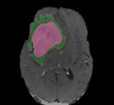
8 Y. Shen et al.
metrics of sensitivity, specificity and dice score. We perform data ablation ex-
periments by substituting our ACM in Eq.11 with standard cross-entropy loss.
The comparison of our proposed methods with the one without ACM loss is
shown in Table 2. The trainable active contour model would increase perfor-
mance on the same U-Net structure.
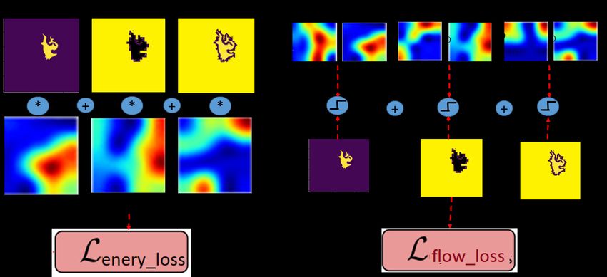
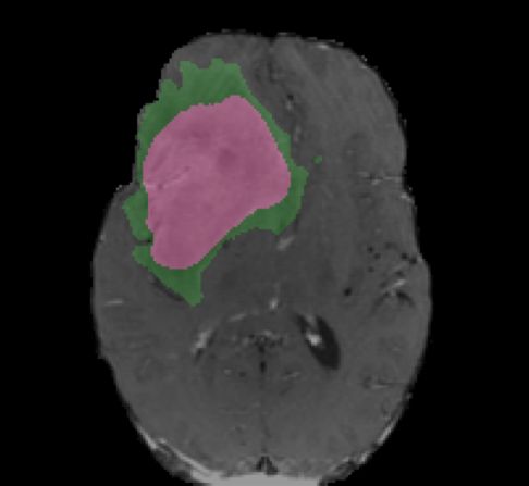
Ground Truth Iteration 1 Iteration 5 Iteration 10
! = 0.5
! = 0.3
! = 0.5
enhanced core
non-enhanced core ! = 0.3
edema
Fig. 4. Segmentation results with various number of iterations and level set thresholds.
3.2 Qualitative Results
Fig. 4 shows the active contours evolving with different number of iterations and
different level set thresholds. The figure shows two examples with one iteration,
five iterations, and ten iterations, and with level set thresholds of 0.5 and 0.3,
respectively. Increasing the number of iterations tends to have smoothing effects
of the boundaries and filtering outlying dots and holes. Changing the level set
threshold values would cause a trade-off between specificity and sensitivity. The
combination of deep learning models and active contour models provides the
flexibility to adjust the results.
4 Conclusion
We propose an active contour model with deep U-Net extracted features. Our
model is trainable end-to-end on an energy minimization function with flow-
regularized optimal constraints. In the experiments, we show that the perfor-
mance of our methods is comparable with state-of-the-art. And we also demon-
strate how the segmentation evolves with the number of iterations and level set
thresholds.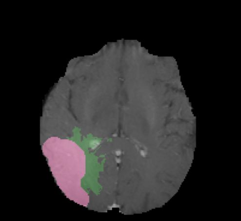
Flow Regularized Model for Brain Tumor Segmentation            9

References
 1. T. F. Chan, S. Esedoglu, and M. Nikolova. Algorithms for finding global min-
    imizers of image segmentation and denoising models. SIAM journal on applied
    mathematics, 66(5):1632–1648, 2006.
 2. T. F. Chan and L. A. Vese. Active contours without edges. IEEE Transactions on
    image processing, 10(2):266–277, 2001.
 3. L. Chen, Y. Wu, A. M. DSouza, A. Z. Abidin, A. Wismüller, and C. Xu. MRI
    tumor segmentation with densely connected 3D CNN. In Medical Imaging 2018:
    Image Processing, volume 10574, page 105741F. International Society for Optics
    and Photonics, 2018.
 4. L. D. Cohen. On active contour models and balloons. CVGIP: Image understand-
    ing, 53(2):211–218, 1991.
 5. R. Dey and Y. Hong. Compnet: Complementary segmentation network for brain
    mri extraction. In International Conference on Medical Image Computing and
    Computer-Assisted Intervention, pages 628–636. Springer, 2018.
 6. P.-A. Ganaye, M. Sdika, and H. Benoit-Cattin. Semi-supervised learning for seg-
    mentation under semantic constraint. In International Conference on Medical
    Image Computing and Computer-Assisted Intervention, pages 595–602. Springer,
    2018.
 7. D. M. Greig, B. T. Porteous, and A. H. Seheult. Exact maximum a posteriori
    estimation for binary images. Journal of the Royal Statistical Society: Series B
    (Methodological), 51(2):271–279, 1989.
 8. K. Kamnitsas, L. Chen, C. Ledig, D. Rueckert, and B. Glocker. Multi-scale 3d
    cnns for segmentation of brain lesions in multi-modal mri, in proceeding of isles
    challenge. MICCAI, 2015.
 9. K. Kamnitsas, C. Ledig, V. F. Newcombe, J. P. Simpson, A. D. Kane, D. K. Menon,
    D. Rueckert, and B. Glocker. Efficient multi-scale 3d cnn with fully connected crf
    for accurate brain lesion segmentation. Medical image analysis, 36:61–78, 2017.
10. Z. Karimaghaloo, D. L. Arnold, and T. Arbel. Adaptive multi-level conditional
    random fields for detection and segmentation of small enhanced pathology in med-
    ical images. Medical image analysis, 27:17–30, 2016.
11. M. Kass, A. Witkin, and D. Terzopoulos. Snakes: Active contour models. Inter-
    national journal of computer vision, 1(4):321–331, 1988.
12. T. H. N. Le, R. Gummadi, and M. Savvides. Deep recurrent level set for segment-
    ing brain tumors. In International Conference on Medical Image Computing and
    Computer-Assisted Intervention, pages 646–653. Springer, 2018.
13. O. L. Mangasarian. Nonlinear programming. SIAM, 1994.
14. B. H. Menze, A. Jakab, S. Bauer, J. Kalpathy-Cramer, K. Farahani, J. Kirby,
    Y. Burren, N. Porz, J. Slotboom, R. Wiest, et al. The multimodal brain tumor
    image segmentation benchmark (brats). IEEE transactions on medical imaging,
    34(10):1993–2024, 2014.
15. Y. Qin, K. Kamnitsas, S. Ancha, J. Nanavati, G. Cottrell, A. Criminisi, and
    A. Nori. Autofocus layer for semantic segmentation. In International Conference
    on Medical Image Computing and Computer-Assisted Intervention, pages 603–611.
    Springer, 2018.
16. H. Spitzer, K. Kiwitz, K. Amunts, S. Harmeling, and T. Dickscheid. Improv-
    ing cytoarchitectonic segmentation of human brain areas with self-supervised
    siamese networks. In International Conference on Medical Image Computing and
    Computer-Assisted Intervention, pages 663–671. Springer, 2018.
10 Y. Shen et al.
17. J. Yuan, E. Bae, and X.-C. Tai. A study on continuous max-flow and min-cut
approaches. In 2010 ieee computer society conference on computer vision and
pattern recognition, pages 2217–2224. IEEE, 2010.
18. C. Zhou, C. Ding, Z. Lu, X. Wang, and D. Tao. One-pass multi-task convolutional
neural networks for efficient brain tumor segmentation. In International Conference
on Medical Image Computing and Computer-Assisted Intervention, pages 637–645.
Springer, 2018.You can also read