Investigation of the Lattice Boltzmann SRT and MRT Stability for Lid Driven Cavity Flow
←
→
Page content transcription
If your browser does not render page correctly, please read the page content below
International Journal of Materials, Mechanics and Manufacturing, Vol. 2, No. 4, November 2014
Investigation of the Lattice Boltzmann SRT and MRT
Stability for Lid Driven Cavity Flow
E. Aslan, I. Taymaz, and A. C. Benim
dynamics for simulation complex flow problems.
Abstract—The Lattice Boltzmann Method (LBM) is applied The simplest LBE is the Lattice Bhatnagar-Groos-Krook
to incompressible, steady, laminar flow high Reynolds numbers (LBGK) equation, based on a Single Relaxation Time
varying in a range from 200 to 2000 for determining stability (LBM-SRT) approximation [4]. Due to extreme simplicity,
limits of the LBM Single Relaxation Time (LBM-SRT) and the
LBM Multiple Relaxation Time (LBM-MRT). The lid driven
the LBGK equation has become most popular Lattice
cavity flow is analyzed. The effect of the model Mach number on Boltzmann equation in spite of its well-known deficiencies,
accuracy is investigated by performing computations at for example, flow simulation at high Reynolds numbers [5].
different Mach numbers in the range 0.09 – 0.54 and comparing Flow simulation at high Reynolds numbers, collision
the results with the finite-volume predictions of the frequency ( ) which is the main ingredient of the LBM-SRT,
incompressible Navier-Stokes equations. It is observed that the
exhibits a theoretical upper bound ( 2 ) that is related with
Mach number does not affect the results too much within this
range, and the results agree well with the finite volume solution the positiveness of the molecular kinematic viscosity [6].
of the incompressible Navier-Stokes equation. LBM-MRT is Thus, stability problems arise as the collision frequency
more stable than LBM-SRT especially for low Mach and high approaches to this limiting value [7]. For incompressible
Reynolds numbers. For the LBM-SRT solutions, collision flows, the flow velocities are limited, since the model
frequency ( ) decreases with increasing Reynolds and Mach immanent Mach number needs to be kept sufficiently small.
numbers, however, for the LBM-MRT solutions, 7th and 8th
Therefore, a lowering kinematic viscosity, for achieving high
relaxation rates ( s7 s8 ) decrease with decreasing Reynolds
Reynolds numbers for a given geometry, pushes the collision
numbers and with increasing Mach numbers. Within its
frequency towards the above-mentioned stability limit. It is
stability range, the convergence speed of the LBM-SRT is
higher (approximately %10) than that of LBM-MRT, while the possible to increase the value of ω by decreasing the size of
convergence speed of the finite volume method is much lower lattices, however, it needs more computer resources [8].
than the both LBM formulations (the LBM-SRT and the Alternatively, using LBM-MRT increases stability limit
LBM-MRT). and resolve the mentioned issue [9]-[17].
In the literature, there are comparative studies of the
Index Terms—Lid driven cavity flow, lattice Boltzmann LBM-SRT and the LBM-MRT for lid driven cavity flows
method, single relaxation time, multiple relaxation time.
[2]-[18]. Those studies find that, the LBM-MRT is superior to
the LBM-SRT at higher Reynolds number flow simulations,
especially for numerical stability. Also, the LBM-SRT and
I. INTRODUCTION the LBM-MRT produces accurate results for all Reynolds
numbers. In addition that, the code using the LBM-MRT
The Lattice Boltzmann equation (LBE) using relaxation
takes only 15% more CPU time than using the LBM-SRT.
technique was introduced by Higuera and Jimenez [1] to cope
In the previous work [2], [18], [19], LBM-SRT and
some drawbacks of Lattice Gas Automata (LGA) such as
LBM-MRT were compared, basically, for the accuracy issues.
large statistical noise, limited range of physical parameters,
The stability properties were not explicitly addressed, besides
non-Galilean invariance and difficult implementation in three
a qualitative statement that LBM-MRT is more stable than the
dimension problem [2]. In the original derivation of LBE
LBM-SRT. The originality of the present investigation
using relaxation concept, it was strongly connected to the
compared to the previous work [2], [18], [19] lies especially
underlying LGA. However, it was soon recognized that it
therein that the stability properties of LBM-SRT and
could be constructed independently [3]. After that, the Lattice
LBM-MRT are systematically and quantitatively compared
Boltzmann Method (LBM) has received considerable
over a large range of Reynolds and Mach numbers.
attention as an alternative to conventional computational fluid
Furthermore, for a better overall assessment of the accuracy,
stability and convergence issues, the results are always
Manuscript received February 5, 2014; revised April 4, 2014. compared with those of the well-established CFD code
E. Aslan is with the Department of the Mechanical Engineering, Istanbul ANSYS-Fluent [20]. In the LBM-SRT, the collision
University, 34320, Istanbul, Turkey (e-mail: erman.aslan@istanbul.edu.tr).
I. Taymaz is with the Department of the Mechanical Engineering, frequency, and in the LBM-MRT, the 7th and 8th relaxation
Sakarya University, 54187, Sakarya, Turkey (e-mail: rates ( s7 s8 ) are related to the molecular kinematic viscosity.
taymaz@sakarya.edu.tr).
A.C. Benim is with the CFD Lab., Department of Mechanical and Process
Therefore, collision frequency and 7th relaxation rate are
Engineering, Duesseldorf University of Applied Sciences, Josef-Gocklen compared with changing Reynolds and Mach number as a
Str.9, 40474, Duesseldorf, Germany (e-mail: stability limits of the LBM-SRT and the LBM-MRT
alicemal.benim@fh-duesseldorf.de).
respectively. Other relaxation times ( s0 , s1 ,..., s6 ) for the
DOI: 10.7763/IJMMM.2014.V2.149 317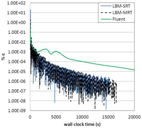
International Journal of Materials, Mechanics and Manufacturing, Vol. 2, No. 4, November 2014
LBM-MRT are taken from Razzaghian et al.,’s study [18], 3 9 3
feq x, t w 1 2 e u 4 e u 2 u u
2
(3)
their work is taken as a reference in investigation of c 2c 2c
LBM-MRT stability limits.
where w is a weighting factor, is the density, u is the
II. NUMERICAL METHODS fluid velocity and c x t , for square lattice, is the lattice
speed, and x ( x y ), t are the lattice length and time
A. LBM with Single Relaxation Times (LBM-SRT) step size. In addition, the discrete velocities for D2Q9 lattice
The lattice Boltzmann method is only applicable to the low model are
Mach number hydrodynamics, because a small velocity
expansion is used in derivation of the Navier-Stokes equation 0 1 0 1 0 1 1 1 1
from lattice Boltzmann equation. It should be noted that the e c (4)
0 0 1 0 1 1 1 1 1
small Mach number limit is equivalent to incompressible limit
[21].
and the values of weighting vectors w are
The LBM method solves the microscopic kinetic equation
for the particle distribution f x, v, t , where x and v is the
4 9 for 0
particle position and the velocity vector respectively, in phase
w 1 9 for 1, 2,3, 4 (5)
space x, v and time t , where the macroscopic quantities 1 36 for 5, 6, 7,8
which are velocity and density are obtained through moment
integration of f x, v, t . The macroscopic values are obtained from the following
The discrete LBM-SRT equation, which is usually solved equations.
in two consecutive steps, i.e. in a “collision” and a following
“streaming” step as provided below. 8 8
f feq (6)
Collision step: 0 0
f x, t t f x, t f x, t feq x , t
8 8
1 1
(1) u e f e f
0 0
eq
(7)
Streaming step: P cs2 (8)
f x e t , t t f x, t t (2) where P is the pressure and cs c 3 is the lattice speed of
sound. The viscosity of the simulated fluids is defined by
Note that, in the above “ ” denotes the post-collision
values. It is obvious that collision process is completely 1 1 2
t cs (9)
localized, and the streaming step requires little computational 2
effort by advancing the data from neighboring lattice points.
In (Eq. 1), f x, t and feq x, t are the particle With the same way, collision frequency can be defined
distribution function and equilibrium particle distribution
as 1 cs2 t 1 2 . The time step size t is chosen in
function of the α-th discrete particle velocity v , e is a
such a way to result in a lattice speed c is unity, resulting in a
discrete velocity vector, and t / is the collision
frequency. Note that is the collision relaxation time. lattice speed sound of cs 1 3.
The 2-dimensional and 9-velocity (D2Q9) lattice model B. LBM with Multiple Relaxation Times (LBM-MRT)
(Fig. 1) is used in the current study for simulating the steady
As mentioned before, LBM with Multi Time Relaxation
lid driven cavity flow. The proposed D2Q9 lattice model
can improve the numerical stability of the LBM. The
obeys also incompressible limit. For isothermal and
LBM-MRT collision model of Q velocities on a
incompressible flows, the equilibrium distribution function
can be derived as the following form [21]. D -dimensional lattice is written as [9]-[16].
f x e t , t t f x, t M1 Sˆ m x , t meq x, t (10)
where M is a Q Q matrix which linearly transforms the
distributions functions f to the velocity moments m .
m Mf and f M1 m (11)
the total number of discrete velocities Q 1 b or b for
model with or without particle of zero velocity, respectively.
Fig. 1. D2Q9 lattice model.
318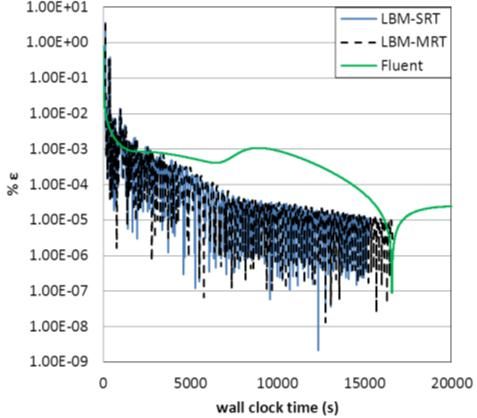
International Journal of Materials, Mechanics and Manufacturing, Vol. 2, No. 4, November 2014
Ŝ is a non-negative Q Q diagonal relaxation matrix, and are;
1 1 2 t 1 1
the bold-face symbols denote the column vectors t cs , cs2 (17)
7
s 2 2 s1 2
f x e t , t t
(12a) For D2Q9 lattice model, it is required that s7 s8
f 0 x e t , t t ,..., f b x e t , t t
T
and s4 s6 . Obviously the relaxation rates s0 , s3 and s5 for
f x, t f 0 x, t ,..., fb x, t
T
(12b) the conserved moments ( , jx , j y ) have no effect for the
m x, t m0 x, t ,..., mb x , t model.. The other relaxation rates, s2 (for ) and
T
(12c)
s4 s6 (for qx and q y ) do not affect the hydrodynamics in the
meq x, t m0eq x, t ,..., mbeq x, t
T
(12d)
lowest order approximation and only affect the small scale
behavior of the model. Also, the relaxation rates ( s4 s6 ) can
where T is transpose operator.
affect the accuracy boundary conditions [22], [23].
For D2Q9 lattice model, moments are listed below,
The LBM-MRT model can reproduce the same viscosity
with the LBM-SRT model, if we set s7 s8 . And, the rest
m , e, , jx , qx , j y , q y , pxx , p yy
T
(13)
of the relaxation parameters ( s1 , s2 , s4 and s6 ) can be
chosen more flexibly [11].
where is the density, and jx ux and j y u y are x As we mentioned before, in the LBM-MRT calculations,
and y components of the flow momentum, respectively, the study of Razzaghian et al. [18] is taken as a reference
which are the conserved moments in the system. Other study, Thus, we will use s0 s3 s5 1 , s1 s2 1.4 ,
moments are non-conserved moments and their equilibria are s4 s6 1.2 and s7 s8 for LBM-MRT calculations.
functions of the conserved moments in the system [9]-[16]. And, we will compare the stability limits of the LBM-SRT
With this particular order of moments given above, the and LBM-MRT using collision frequency ( ) and 7th
corresponding diagonal relaxation matrix of relaxation rates. relaxation rate ( s7 s8 ) for lid driven cavity flow,
respectively.
Ŝ diag s0 , s1 , s2 , s3 , s4 , s5 , s6 , s7 , s8
(14)
diag s , se , s , s jx , sqx , s j y , sq y , s pxx , s pxy
III. RESULTS AND DISCUSSION
The equilibria of the non-conserved moments A. Lid Driven Cavity Flow
The lid driven cavity flows are investigated. The geometry
m1eq eeq 2 3 jx2 j y2 , and boundary conditions of the lid driven cavity flow are
(15a)
m2eq eq 3 jx2 j y2
sketched in Fig. 2. Where u x and u y are x and y
component of the flow velocity, and u0 is the boundary value.
m4eq qxeq jx , m6eq qxeq j y , (15b) Computations are performed for Reynolds numbers (Re),
m p j j
eq
7
eq
xx
2
x
2
y ,m eq
8 p jx j y
eq
xy (15c) which are based on inlet velocity (u0) and hydraulic diameter
(H) varying within the range 200 and 2000. Mach numbers
(Ma) which are based on inlet velocity (u0) and speed of
with the orderings of the discrete velocities and
sound (cs) are varied between 0.09 and 0.54. In order to
corresponding moments given above for D2Q9 lattice model,
acquire Mach numbers, inlet velocities are varied between
the transform matrix M in (10) is
0.0519 and 0.3117. For each computation, various values of
the collision frequency ( ) for LBM-SRT and 7th and 8th
1 1 1 1 1 1 1 1 1
relaxation rates ( s7 s8 ) for LBM-MRT are used, for
4 1 1 1 1 2 2 2 2
detecting the highest possible value for a stable solution.
4 2 2 2 2 1 1 1 1
0 1 0 1 0 1 1 1 1
M 0 2 0 2 0 1 1 1 1 (16)
0 0 1 0 1 1 1 1 1
0 0 2 0 2 1 1 1 1
0 1 1 1 1 0 0 0 0
0 0 0 0 0 1 1 1 1
For D2Q9 lattice model, the shear viscosity , which is
same in (Eq. 9), but in this formula, 7th and 8th relaxation rates
used instead of collision frequency and the bulk viscosity Fig. 2. Lid driven cavity flow.
319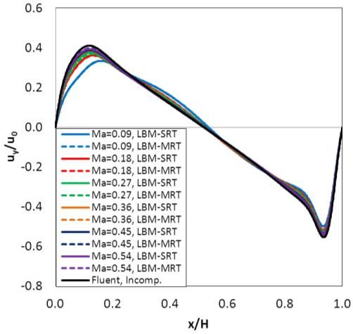
International Journal of Materials, Mechanics and Manufacturing, Vol. 2, No. 4, November 2014

                                                                                figure, LBM-SRT and LBM-MRT predictions are very close
                                                                                each other.
                                                                                   Fig. 4 displays the predicted contours of nondimensional
                                                                                u x velocity component for Re=2000 and lid driven cavity
                                                                                flow, predicted for different Mach numbers, and for the
                                                         (a)
                                                                                LBM-SRT and LBM-MRT. The main recirculation structure
                                                                                gets more symmetric for Re=2000, as expected based on
                                                                                previous studies on this typical benchmark flow problem
                                                                                Comparing the solution for Re=2000, one can see that Mach
                                                                                number variations within the considered range does not
                                                                                remarkably affect from the flow field for LBM-SRT and
                                                                                LBM-MRT. Additionally, there is unnoticeable difference
                                                                                between predictions of LBM-SRT and LBM-MRT

                                                         (b)

                                                                                                                                          (a)

                                                         (c)

                                                                                                                                          (b)

                                                         (d)

                                                                                                                                          (c)

  Fig. 3. LBM predicted non dimensional velocity ( ux u0 ) contours for
Re=200 and lid driven cavity flow: (a) LBM-SRT, Ma=0.09, (b) LBM-MRT,
     Ma=0.09, (c) LBM-SRT, Ma=0.54, (d) LBM-MRT, Ma=0.54.

    Incompressible LBM formulations are used both
LBM-SRT and LBM-MRT. Ansys-Fluent discretizes the
incompressible Navier-Stokes equations with Finite Volume
Method. Therefore, for validation LBM results,
well-established CFD code, Ansys-Fluent is used. The same                                                                                 (d)
mesh sizes are used, of course, for validation
    Fig. 3 displays the predicted contours of nondimensional
 u x velocity component for Re=200 and lid driven cavity flow,
predicted for different Mach numbers, and for the LBM-SRT
and the LBM-MRT. Comparing the solution for Re=200, one
can see that Mach number variations within the considered                         Fig. 4. LBM predicted non dimensional velocity ( ux u0 ) contours for
range does not remarkably affect from the flow field for the                       Re=2000 and lid driven cavity flow: (a) LBM-SRT, Ma=0.09, (b)
LBM-SRT and the LBM-MRT. As also can be seen from the                           LBM-MRT, Ma=0.09, (c) LBM-SRT, Ma=0.54, (d) LBM-MRT, Ma=0.54.

                                                                          320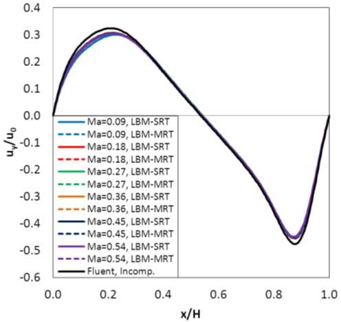
International Journal of Materials, Mechanics and Manufacturing, Vol. 2, No. 4, November 2014
(a) (a)
(b) (b)
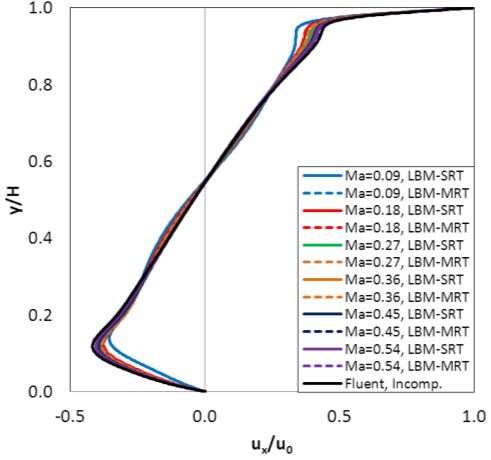
Fig. 5. Non dimensional velocity profiles for Re=200, (a) u x velocity at Fig. 7. Non dimensional velocity profiles for Re=1000,
(a) u x velocity at x=H/2, (b) u y velocity at y=H/2.
x=H/2, (b) u y velocity at y=H/2.
(a) (a)
(b) (b)
Fig. 6. Non dimensional velocity profiles for Re=500, (a) u x velocity at Fig. 8. Non dimensional velocity profiles for Re=2000,
(a) u x velocity at x=H/2, (b) u y velocity at y=H/2.
x=H/2, (b) u y velocity at y=H/2.
321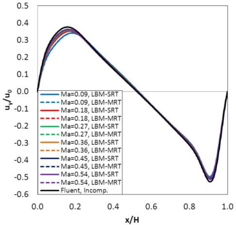
International Journal of Materials, Mechanics and Manufacturing, Vol. 2, No. 4, November 2014
Fig. 5(a) compares the predicted u x velocity profiles along the maximum allowed value beyond which the solution
a vertical line at x/H=1/2 for Re=200. The u y velocity becomes unstable, i.e, no converged steady-state solution can
be obtained. Theoretically, it is obvious that the collision
profiles for the same Reynolds number, along a horizontal
frequency or 7th (or 8th) relaxation rates are not allowed to
line at y/H=1/2 are compared in Fig. 5(b). In Fluent
take the value 2, but needs to be smaller.
computations, 2nd Order Upwind scheme have been used as
discretization scheme. Fluent and all LBM predictions are
displayed in the figures. One can see that the all LBM
predictions (from Ma=0.09 and Ma=0.54) are quite close
each other and agree very well with the Fluent predictions for
Re=200.
Fig. 6(a), Fig. 7(a) and Fig. 8(a) present the predicted u x
(a)
velocity profiles along a vertical line at x/H=1/2 for Re=500,
1000 and 2000 respectively. The predicted u y velocity
profiles along a horizontal line at y/H=1/2 are compared in
Fig. 6(b), Fig. 7(b) and Fig. 8(b) for Re=500, 1000 and 2000
respectively. One can see from the figures that as the
Reynolds number increases, the difference between the LBM
and Fluent predictions becomes larger. The largest
differences between the LBM and the Fluent computations
are observed at Ma=0.09 for all Reynolds number. As it can
also be seen from the figures, for all Reynolds numbers and all
Mach numbers, the predictions of the LBM-SRT and the
LBM-MRT are quite close each other.
(b)
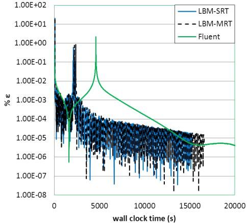
Based on the lid driven cavity flow, converge behaviors of
the present LBM-SRT and LBM-MRT code and Fluent are
also compared in Fig. 9, for Re=1000 and Ma=0.27. For a
better comparability, the same criteria, namely the percentage
variation (which indicated as % ε in the figures) of a variable
at a given monitor point is taken as the indicator of the
convergence, for all codes. For general variable (which
can be u x or u y ), this is computed from
n 1 n
% 100 (18)
n
In (18), the parameter n denotes the iteration number. (c)
Obviously, the same grids are used, and computations are
started from the same initial velocity field distributions (zero
velocity everywhere in the flow field). Of course, the same
computer is used for all computations. For the Fluent
computations, the Simple pressure-correction procedure is
used. For the under relaxation factors, the default values are
applied for all variables [20]. As can be seen in Fig. 9, both
Lattice Boltzmann computations (the LBM-SRT and the
LBM-MRT) show, in general, a better overall convergence
rate (according to present definition described by (Eq.18)).
On the other hand, all the Lattice Boltzmann Method results
exhibit some “wiggles” along the way of convergence. The
(d)
residuals obtained by the Ansys-Fluent code exhibit a more
smooth behavior. As it can also be seen in Fig. 9, converge of
the LBM-SRT is achieved approximately %10 earlier than the
LBM-MRT.
B. Stability Limits
For a range of Reynolds ( 200 Re 2000 ), and Mach
( 0.09 Ma 0.54 ) numbers, different values of collision Fig. 9. Converge behavior (Re=1000 and Ma=0.27): (a) % ε in u x at x=H/2,
frequency ( ) for the LBM-SRT and 7th and 8th relaxation y=3H/4, (b) % ε in u x at x=H/2, y=H/4, (c) % ε in u y at x=H/4, y=H/2,
rates ( s7 s8 ) for the LBM-MRT are applied, for detecting (d) % ε in u y at x=3H/4, y=H/2.
322
International Journal of Materials, Mechanics and Manufacturing, Vol. 2, No. 4, November 2014
For the LBM-SRT, the predicted maximum allowed TABLE I: COEFFICIENTS a1 Re AND a2 Re OF (19)
collision frequency for a stable solution (the solid lines) are LBM-SRT
presented in Fig. 10, as a function of Mach number, for a1 0.018ln Re 0.396
different values of the Reynolds number. As can be seen from
a2 0.002ln Re 1.7897
Figure 10, the maximum allowed collision frequency ( )
values decrease with Reynolds number, whereas for a given
Reynolds number, also a decrease with the Mach number is For the LBM-MRT calculations, the curves mostly exhibit
predicted. a 2nd order polynomial like variation with the Mach number.
Therefore, a trial has been presented to fit a 2 nd order
polynomial curve to the predicted data, the coefficients being
functions of the Reynolds number, which can be expressed as;
s7, MAX s8, MAX b1 Re Ma 2 b2 Re Ma b3 (20)
The coefficients b1 Re , b2 Re and b3 Re of (20),
which are obtained by curve fitting to the predicted data are
presented in Table 2. The 2nd order polynomial curves predict
by (20) are also displayed in Fig. 11, as the dashed lines,
where corresponding legends are designated by the suffix “cf”
after the corresponding Re value,
Fig. 10. Predicted maximum values (LBM-MRT) for stable solution: TABLE II: Coefficients b1 Re , b2 Re and b3 Re of (20)
The dashed lines and suffix “cf” refer to the curve of (19) and Table I.
LBM-MRT
For the LBM-MRT, the predicted maximum 7 and 8 th th b1 0.26ln Re 1.1415
relaxation rates for a stable solution (the solid lines) are b2 0.04856ln Re 3.3577
presented in Fig. 11, as a function of Mach number, for
b3 0.048ln Re 2.2777
different values of Reynolds number. The maximum 7th and
8th relaxation rates increase with increasing Reynolds number
and with decreasing Mach number.
The curves mostly exhibit a linear like variation with the IV. CONCLUSION
Mach number for the LBM-SRT calculations. Thus, a trial has Incompressible steady state formulations of the LBM-SRT
been given to fit a linear curve to the predicted data, the and the LBM-MRT are applied to laminar flows for Reynolds
coefficients being functions of the Reynolds number, which numbers between 200 and 2000, where the Mach number is
can be expressed as; also varied between 0.09 and 0.54. The lid driven cavity flow
problem is analyzed. Stability limits, in terms of the maximum
MAX a1 Re Ma a2 Re (19)
allowed collision frequency ( ) for LBM-SRT and 7th and
The coefficients a1 Re and a2 Re of (19), which are 8th relaxation rates ( s7 s8 ), as a function of Reynolds and
obtained by curve fitting to the predicted data are presented in Mach numbers are explored. It is observed that, for low Mach
Table I. The linear curves predict by (19) are also displayed in and high Reynolds number the LBM-MRT is more stable than
Fig. 10, as the dashed lines, where corresponding legends are LBM-SRT. Collision frequency decreases with increasing
designated by the suffix “cf” (for “curve fitting”) after the Reynolds and Mach numbers for the LBM-SRT. However, 7th
corresponding Re value. and 8th relaxation rates decrease with decreasing Reynolds
numbers and with increasing Mach numbers. Comparisons
with the general purpose, finite-volume based CFD code,
using incompressible formulation has served as a validation
of the present Lattice Boltzmann Method (both the LBM-SRT
and the LBM-MRT) based code, at the same time confirming
that the present incompressible Lattice Boltzmann
formulation predicts flow field that behave sufficiently
incompressible for the considered range of Mach numbers.
Also, converge behavior of the both Lattice Boltzmann codes
(both LBM-SRT and LBM-MRT) and finite volume based
CFD code are explored. It is observed that, all Lattice
Boltzmann codes are much faster than finite volume based
CFD code. Also, convergence speed of the LBM-SRT is
Fig. 11. Predicted maximum s7 ( s7 s8 ) values (LBM-MRT) for stable better (approximately %10) than LBM-MRT with using same
solution: The dashed lines and suffix “cf” refer to the curve of (20) and Table grid size.
2.
323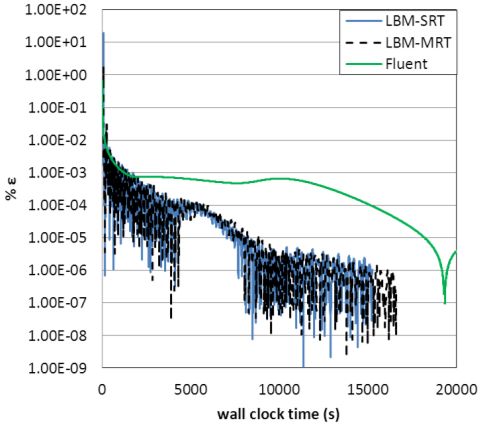
International Journal of Materials, Mechanics and Manufacturing, Vol. 2, No. 4, November 2014

                               REFERENCES                                                      2012 International Conference on Fluid Dynamics and Technologies,
                                                                                               Singapore, 2012, pp. 130-135.
[1]    F.J. Higuera and J. Himenez, “Boltzmann Approach to Lattice Gas                  [18]   M. Razzaghian, M. Pourtousi, and A. N. Darus, “Simulation of flow in
       Simulation,” Europhysics Letter, vol. 9, pp. 663-668, 1989.                             lid driven cavity by MRT and SRT,” in Proc. International
[2]    J. S. Wu and Y. L. Shao, “Assessment of SRT and MRT scheme in                           Conference on Mechanical and Robotics Engineering, Phuket, 2012,
       parallel lattice boltzmann method for lid-driven cavity flows,” in Proc.                pp. 94-97.
       the 10th National Computational Fluid Dynamics Conference,                       [19]   J. S. Wu and Y. L. Shao, “Simulation of lid driven cavity flow by
       Hua-Lien, 2003.                                                                         parallel lattice boltzmann method using multi relaxation time scheme,”
[3]    F. J. Higuera, S. Succi, and R. Benzi, “Lattice gas-dynamics with                       International Journal for Numerical Methods in Fluids, vol. 46, pp.
       enchanced,” Europhysics Letter, vol. 9, pp. 345-349, 1989.                              921-937, 2004.
[4]    P. L. Bhatnagar, E. P. Groos, and M. Krook, “A model for collision               [20]   Ansys-Fluent 12.0 Users’s Guide, Ansys Inc., 2009.
       process in gases I. small amplitude process in charged and neutral one           [21]   X. He and L. S. Luo, “Lattice boltzmann model for incompressible
       component system,” Physical Review, vol. 94, pp. 511-525, 1954.                         navier-stokes equation” Journal of Statiscal Physics, vol. 88, no. 3-4,
[5]    Y. Qian, D. D’Humières, and P. Lallemand, “Lattice BGK models for                       pp. 927-944, 1997
       navier-stokes Equation,” Europhysics Letter, vol. 17, pp. 479-484,               [22]   D. A. Wolf-Gladrow, Lattice Gas Cellular Automata and Lattice
       1992.                                                                                   Boltzmann Models, Berlin, Springer, 2005.
[6]    S. Succi, The Lattice Boltzmann Equation for Fluid Dynamics and                  [23]   Y. Peng and L. S. Luo, “A comparative study of Immersed-Boundary
       Beyonds, Oxford, Calderon Press, 2001.                                                  and Interpolated Bounce-back methods, Progress in Computational
[7]    M.       Fink,      “Simulation     von      Nasenströmungen         mit                Fluid Dynamics, vol. 8, no. 1-4, pp. 156-157, 2008.
       Lattice-BGK-Methoden,” Ph.D. dissertation, Essen-Duisburg
       University, Germany, 2007.
                                                                                                               E. Aslan received his BSc, MSc and PhD in
[8]    A. C. Benim, E. Aslan, and I. Taymaz, “Investigation into LBM
                                                                                                               mechanical engineering from the University of
       analyses of incompressible laminar flows at high reynolds numbers,”
                                                                                                               Sakarya, Turkey.
       WSEAS Transactions on Fluid Mechanics, vol. 4, no. 4, pp. 107-116,
                                                                                                                He is currently an assistant professor of Mechanical
       2009.
                                                                                                               Engineering Department at University of Istanbul. He
[9]    D. d’Humières, “Generalized lattice boltzmann equation,” AIAA
                                                                                                               teaches undergraduate and graduate courses. His
       Rarefied Gas Dynamics: Theory and simulations, vol. 159, pp.
                                                                                                               research area fluid mechanics, heat transfer,
       450-458, 1992.
                                                                                                               aerodynamics, numerical methods on fluid flow and
[10]   D. d’Humières, I. Ginzburg, M. Krafczyk, P. Lallemand, and L. S. Luo,
                                                                                                               heat transfer such as Finite Volume Method (FVM)
       “Multiple relaxation time lattice boltzmann models in three                      oto
                                                                                        and LBM.
       dimensions,” Philosophical Transactions The Royal Society London,
       vol. 360, pp. 437-451, 2002.
[11]   P. Lallemand and L. S. Luo, “Theory of the lattice boltzmann method:
                                                                                                               I. Taymaz received his BSc and MSc in mechanical
       dispersion isotropy galilean invariance and stability,” Physical Review
                                                                                                               engineering from the Technical University of Istanbul,
       E, vol. 61, no. 1, pp. 775-719, 2000.
                                                                                                               and his PhD form University of Sakarya, Turkey.
[12]   P. Lallemand and L. S. Luo, “Theory of the lattice boltzmann method:
                                                                                                                  He is currently an associate professor of Mechanical
       acoustic and thermal properties in in two and three dimensions,”
                                                                                                               Engineering Department at University of Sakarya. He
       Physical Review E, vol. 68, pp. 036706-1–036706-25, 2003.
                                                                                                               teaches undergraduate and graduate courses in
[13]   A. A. Mohamad, Lattice Boltzmann Method, Fundementals,
                                                                                                               automotive division. His research areas of interest
       Applications with Computer Codes, London, Springer, 2011.
                                                                                                               include advanced technologies in engines for
[14]   M. A. Moussaoui, A. Mezrhab, H. Naji, and M. E. Gabaoui,
                                                                                                               automotive industry.
       “Prediction of heat transfer in a plane channel built-in three heated
       square obstacles using an mrt lattice boltzmann method,” in Proc. the
                                                                                                               C. Benim received his BSc and MSc in mechanical
       Sixth International Conference on Computational Heat and Transfer,
                                                                                                               engineering from the Bosphorus University of
       Guanzhou, China, 2009, pp.176-181.
                                                                                                               Istanbul, Turkey and his PhD form University of
[15]   M. A. Moussaoui, M. Jami, A. Mezrhab, and H. Naji, “MRT-lattice
                                                                                                               Stuttgart, Germany, in 1988.
       boltzmann simulation of forced convection in a plane channel with an
                                                                                                                  Following a post-doctoral period at the University
       inclined square cylinder,” International Journal of Thermal Sciences,
                                                                                                               of Stuttgart, he joined ABB Turbo Systems Ltd. in
       vol. 49, pp. 131-142, 2010.
                                                                                                               Baden, Switzerland, in 1990. He was the manager of
[16]   H. Yu, L. S. Luo, and S. S. Girimaji, “LES of turbulent square jet flow
                                                                                                               the “Computational Flow and Combustion Modelling”
       using an MRT lattice boltzmann model,” Computers & Fluids, vol. 35,
                                                                                                               group, since January 1996, he is a professor of energy
       pp. 957-965, 2006.
                                                                                                               technology at the Düsseldorf University of Applied
[17]   M. Pourtousi, M. Razzaghian, A. Saftari, and A. N. Darus, “Simulation
                                                                                        Sciences, Germany.
       of fluid flow inside a back-ward-facing step by MRT-LBM,” in Proc.

                                                                                  324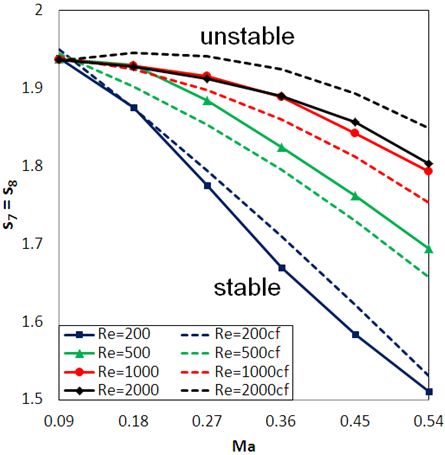
You can also read