An integrative modeling approach to the age-performance relationship in mammals at the cellular scale
←
→
Page content transcription
If your browser does not render page correctly, please read the page content below
www.nature.com/scientificreports

                        OPEN       An integrative modeling
                                   approach to the age-performance
                                   relationship in mammals at the
Received: 24 September 2018
Accepted: 25 November 2018         cellular scale
Published: xx xx xxxx
                                   Geoffroy Berthelot 1,2, Avner Bar-Hen3, Adrien Marck1,4, Vincent Foulonneau1,
                                   Stéphane Douady4, Philippe Noirez1, Pauline B. Zablocki-Thomas5,6, Juliana da Silva Antero1,
                                   Patrick A. Carter7, Jean-Marc Di Meglio4 & Jean-François Toussaint1,8
                                   Physical and cognitive performances change across lifespan. Studying cohorts of individuals in specific
                                   age ranges and athletic abilities remains essential in assessing the underlying physiological mechanisms
                                   that result in such a drop in performance. This decline is now viewed as a unique phenotypic biomarker
                                   and a hallmark of the aging process. The rates of decline are well documented for sets of traits such
                                   as running or swimming but only a limited number of studies have examined the developmental and
                                   senescent phases together. Moreover, the few attempts to do so are merely descriptive and do not
                                   include any meaningful biological features. Here we propose an averaged and deterministic model,
                                   based on cell population dynamics, replicative senescence and functionality loss. It describes the
                                   age-related change of performance in 17 time-series phenotypic traits, including human physical and
                                   cognitive skills, mouse lemur strength, greyhound and thoroughbred speed, and mouse activity. We
                                   demonstrate that the estimated age of peak performance occurs in the early part of life (20.5% ± 6.6%
                                   of the estimated lifespan) thus emphasizing the asymmetrical nature of the relationship. This model
                                   is an initial attempt to relate performance dynamics to cellular dynamics and will lead to more
                                   sophisticated models in the future.

                                   Pierre de Coubertin revived the Olympic Games in 1896. Since then, international sport competitions have
                                   become major events which make evident the progression of human performances over the years1. Practical tools
                                   have been progressively developed to measure human speed and stamina and to explore the underlying physi-
                                   ology of these performance traits2–4. The fast pace of technological innovations now allows for a precise meas-
                                   urement of human performance, such as the top speeds in running events. These measurements extend to other
                                   species used in sport, such as greyhounds and thoroughbreds5,6. The very large amount of recorded data now
                                   allows for the investigation of key questions such as the presence of physical limitations1,5,6. Performance depends
                                   on numerous factors, including genetics7,8, environment (such as ambient temperature)1 and/or technology1. A
                                   leading determinant of performance is the chronological age of the athlete9,10. In humans, decline in physical
                                   performance usually occurs by age 20–309–12, as does working capacity13,14 and other physiological abilities15–20.
                                   Knechtle et al. showed exceptions to this rule; for example, the age-related performance decline starts later in life
                                   for running long distances, possibly because of experience20,21. Increased reaction time, decreased coordination
                                   and joint mobility, decreased skeletal size and muscle bulk, decreased type 2 fast-twitch muscle fibers, changed
                                   body fat composition, and decreased cardiovascular and respiratory functions are among the physiological factors
                                   that are associated with the observed decline11,22,23. Belsky et al. also showed an increasing pace of coordinated

                                   1
                                     Institut de Recherche bio-Médicale et d’Epidémiologie du Sport (IRMES), EA 7329, Institut National du Sport de
                                   l’Expertise et de la Performance (INSEP) and Université Paris Descartes, Sorbonne Paris Cité, Paris, France. 2REsearch
                                   LAboratory for Interdisciplinary Studies (RELAIS), Paris, France. 3CNAM, 75003, Paris, France. 4Laboratoire
                                   Matière et Systèmes Complexes, UMR 7057, Université Paris Diderot and CNRS, Sorbonne Paris Cité, Paris, France.
                                   5
                                     Département de Biologie, ENS de Lyon, Lyon, France. 6Département d’écologie et de Gestion de la Biodiversité,
                                   UMR 7179 CNRS/MNHN, Paris, France. 7School of Biological Sciences, Washington State University, Pullman, USA.
                                   8
                                     CIMS, Hôtel-Dieu, APHP, Paris, France. Correspondence and requests for materials should be addressed to G.B.
                                   (email: geoffroy.berthelot@insep.fr)

        SciEntific RepOrTS |   (2019) 9:418 | DOI:10.1038/s41598-018-36707-3                                                                           1
www.nature.com/scientificreports/
deterioration across multiple organ systems with an exponential increase in physical burden (e.g. pain, fatigue)
from several different chronic conditions after the fifth decade of life24. The rate of physical decline in aging adults
has been studied in various disciplines10–12,25 and is now regarded as a hallmark of the aging process4,26, and serves
as a key indicator of diminishing quality of life while remaining a predictor of physical disability and other mor-
bidities4. Justice et al. argued that functional assessments provide a unique and practical phenotypic biomarker,
as well as a convenient tool to measure response to later life interventions4.
From a broader perspective, the complete lifetime trajectory from young to advanced ages was investigated by
Dan H. Moore for track and field performances27. He showed that the age-related changes of top physical perfor-
mance in 15 running and two throwing events exhibit an inverted-U pattern that can be described using a single
equation based on two non-linear functions:
P(t ) = a(1 − e−bt ) + c(1 − e dt ), P(t ) ≥ 0 (1)
where a, b, c, d are four positive constants and P(t) is the performance value at age t. Equation (1) can be accu-
rately applied to existing datasets in a variety of species10,25,26 for a number of different individual athletic or
cognitive capacities despite inter-individual variability10,25. Other studies have used second-order polynomial
equations to fit the pattern9; however, the age-performance relationship is consistently reported to be asymmet-
rical, with an ‘early’ (i.e. before mid lifespan) age of peak performance10,25–27, meaning that quadratic functions,
such as second order polynomials, provide a poor estimate of the age of peak performance.
Working at The Cellular Scale
The equations used to describe the age-related physical performance, such as Eq. (1), are designed from a statisti-
cal and empirical perspective and do not include any biological or physiological assumption(s) in their approach
(e.g., the four constants in Eq. (1) do not have a particular biological meaning). In fact, excluding biological
assumptions often leads to peculiar equations, such as Eq. (1) that separates the growing (maturation) from the
declining (aging) process. Moreover, such relationships must be driven by developmental changes and senescence
in physiological systems. Muscle mass, body mass and height, oxygen uptake, hormones and other physiological
parameters progressively change with age to allow for an increase in performance from infancy to adulthood.
Likewise, a functional decrease then progressively takes place, affecting such physiological factors as lung volume,
muscle width, testosterone index, etc., resulting in declining performance at older ages26. Importantly, most of
these physiological parameters are determined by mechanisms occurring at the cellular level. The cell is a fun-
damental biological unit of all known living organisms, suggesting that the cellular scale is useful for developing
inter-specific models of age-related physical performance.
In terms of cell dynamics, population models can typically be used to describe cell replication, proliferation
and death. In particular, the well-known Siler model28:
q(t ) = a1. e−b1t + a2 + a3. e b 3t (2)
describes mortality dynamics, with the total hazard function q(t) depending on age-related hazards a1,b1 (immature
animals), a2,b2 (mature animals), a3,b3 (senescence). Interestingly, Eq. (2) becomes Eq. (1) -i.e. q(t ) = a1(1 − e−b1t )
+a3(1 − e b 3t )- when the constant hazard for mature animals is changed to an age-dependent hazard with value
a2 ≡ a2(t ) = a1 + a3 − 2a1e−b1t − 2a3e b 3t. This is similar to the Heligman and Pollard (HP) approach based on the
typical Gompertz law for modeling age-related mortality29. Using Siler approach, parameters a, b, c, d of Eq. (1) can
now be interpreted as the initial hazard for immature (a1 ≡ a) or mature (a3 ≡ c ) animals and 1/b1,3 are the two time
constants with which the immature (b1 ≡ b) and mature (b3 ≡ d ) hazards are reduced. Both Siler and HP models
include predation and a countable number of developmental phases in which hazards occur, limiting their scope of
application. However, models that describe population dynamics provide a guide for the design of a bottom-up
approach to the age-performance relationship of multiple species at the cellular level. In particular, the Siler and Moore
analogy is interesting as it lays the foundations for defining a general model of lifetime changes in performance.
Objectives
Here we aim to introduce a model that is a first step in describing the biological basis of the asymmetrical and
inverted-U pattern typically seen in performance curves. The motivation is to link organismal performance to
the elementary units on which it relies: cells. We will use a population approach to model the observed perfor-
mance patterns while defining cells as the elementary component of the organism. This new model is designed to
be simple and expandable. We test the model for a variety of physiological functions and species, including five
terrestrial mammals (human, thoroughbred, greyhound, mouse, mouse lemur).
Materials and Methods
We define performance P(t) as the measurable outcome of a given system. The measured speed of an individual
in a 100 m track and field event, the crawling speed of a snail, the distance jumped by a frog, the lactation perfor-
mance (i.e., milk production) of a cow are such examples of performance. We assume that the observed perfor-
mance results from the contribution of all the elementary components to the system.
General model of lifetime changes in performance. Consider a population of N cells that grow during
the development phase. Population models, such as Eq. (2), provide some useful guides to handle the dynamics
of N: first, we shall consider that the detrimental processes occurring with aging progressively appear with time
in a continuous manner. Hazards in Siler & HP approaches are also continuously related to time through three
different stages of life (as in Eq. (2)). Second, in Siler & HP approaches, hazards are additive and non-interacting.
SciEntific RepOrTS | (2019) 9:418 | DOI:10.1038/s41598-018-36707-3 2www.nature.com/scientificreports/
We choose a similar formalization for the preliminary model presented here because it is simpler to ignore inter-
action. We recognize that performance is a complex process influenced by both emergent physiological processes
as well as cell traits. For the purposes of this approach, we chose to simplify the model and therefore focus on the
cell scale because of the difficulty of modeling emergent processes.
The general equation governing the performance with aging P(t) in continuous time, with non-interacting cell
types may then be written as:
dNi(t )
= α i (t )Ni(t )
dt
P(t ) = ∑Φi βi(t )Ni(t )
(3)
i
where Ni(t) is a population of cells of a given type i (neurons, specialized myocytes, etc.), αi(t) is the growth rate,
∑ i Ni = N , the total population of all cells, βi(t) is a senescence parameter that embeds the adverse biological
effects as a simple rate of decline that appears with aging. Parameter c is the contribution of the population of cells
to the observed performance P(t). For example, if the performance measured is speed in m.s−1, then Φi is the
increase in speed per cell.
Empirical studies demonstrate the existence of heterogeneity in performance changes with aging, thus empha-
sizing that both the rate of increase αi(t) and decline βi(t) may differ among cell types30. Three issues arise when
taking into account cell specialization:
• parameter Φi and functions αi(t), βi(t) remain unknown and depend on the cell type. However, it is possible
to roughly infer which particular cell types may matter during a specific task.
• the regeneration/replacement effect that takes place in many cell types: dead cells are partly replaced by new
ones, leading to a variation of N(t) at each time step. We assume that this effect is embedded in βi(t).
• Interactions may occur between different cellular types, leading to joint/cooperative contribution to the per-
formance. As previously mentioned, we ignore interaction in Eq. (3) at this time.
Thus we have focused on a simpler and averaged approach, designed to offer an appropriate trade-off between
tractability and complexity while efficiently describing the chosen time series from a biological perspective.
Integrative model of age-performance (IMAP1). In order to account for holistic biological effects, we
next introduce the Integrative Model of Age Performance (IMAP1) that integrates the dynamics of all cell types
simultaneously. This model will necessarily look very similar to Eq. (3). We focus on the quantity N(t) at time t
and define α(t) and β(t) as two age-related parameters that start at the time of the first cellular division t* with
t ≥ t0 > t* and t0 = 0 years. Parameters α(t) and β(t) are two decreasing functions of time. The first parameter is
the growth rate of the population of cells that includes growth-limiting factors that progressively occur with mat-
uration and limiting body size31 that result in a progressive decline in cell proliferation, leading to an asymptotic
saturation of N(t). The second parameter β(t) is the averaged monotonic age-related rate of decline of functional-
ity of all cells N(t). This is a fundamental process that occurs in all cell types irrespective of specific functionality.
For example, metabolic wastes and protein aggregation are processes known to lead to decreased functionality
in all cell types32; for instance, lipofuscin residues building up in cells are associated with detrimental effects on
functionality in several organs33. These two parameters α(t) and β(t) capture the system behavior as a whole,
integrating the dynamics of all cell types including their respective contributions Φi. The model is formulated as:
dN (t )
= α(t )N (t )
dt
P(t ) = β(t )N (t )
(4)
We can more specifically define α(t), the growth parameter, as
α(t ) = α 0e−αrt (5)
where α 0 = α(t0) > 0, the initial (or baseline) average value of the saturation (i.e. the value at t0), which corre-
sponds to the average time of cellular division of N(t). Parameter αr > 0 is the strength of saturation, which is the
amount of time required to reach the asymptote of cell growth. Based on the known decline of performance with
aging, we assume that β(t), the average age-related decline of cell functionality, has the following form:
β(t ) = β0(1 − e β r(t −td )) (6)
Parameter β0 = β(t0) > 0 is the initial (or baseline) value, βr > 0 the strength of the decline of cell functionality, and
td > 0 is the time of death. Low βr values will lead to a linear decline towards td after the age of peak performance.
Conversely, high values show that the functional capabilities are preserved with aging until a sharp exponential
decrease toward td occurs. Solving Equation (4) for P(t) yields:
α0 −αr t
P(t ) = β0N0 ⋅ e αr (1 −e )
⋅ (1 − e β r(t −td )) (7)
SciEntific RepOrTS | (2019) 9:418 | DOI:10.1038/s41598-018-36707-3 3www.nature.com/scientificreports/
Figure 1. IMAP1 with three sets of parameters values. (a) Green line corresponds to α 0⁎ = 1000, αr⁎ = 100,
βr⁎ = 5, the blue one is α 0⁎ = 50, αr⁎ = 15, βr⁎ = 10 and the red one is α 0⁎ = 200, αr⁎ = 10, βr⁎ = 20. The (b)
panel shows the overall cell population size, reflecting the average proliferation capacity while panel (c) shows
the values embedding adverse effects of senescence, resulting in functionality drop.
where N0 is the initial (or baseline) number of cells at t0. The right side of the equation is similar to the second
component of the right side of Eq. (1) but includes td as the explicit time of death. Equation (7) can also be written
as:
α0 −αr t
P(t ) = β0N∞ ⋅ e− αr e ⋅ (1 − e β r(t −td )) (8)
α0
with the cell population at the asymptote, N∞ = N0e αr . This is a convenient formalization as it reduces the com-
plexity of the multidimensional space and allows for a faster convergence in the search for optimal solutions using
the Levenberg-Marquardt algorithm34. The reduced form of Eq. (8) is:
α 0⁎ −αr⁎u
− e ⁎
x(u ) = e α r⁎ ⋅ (1 − e β r (u −1)) (9)
with u ≡ t , x(u) defining the dimensionless quantity x(u) ≡ P (t ) and α 0⁎ ≡ α 0td , αr⁎ ≡ αr td , βr⁎ ≡ βr td . The
td β 0N∞
behavior of this equation is pictured in Fig. 1 for different parameter values.
Data collection and non-linear regressions. A set of 17 time series were collected from available on-line
sources, previous publications and experimental studies:
• Physical performances in 8 track and field sport events. The speeds in m.s−1 are collected for the 100 m,
400 m, 800 m, 3000 m, 5000 m, 10000 m, marathon and the force momentum (in kg.m) for shot-put events
in men. A total of 57587 performances were collected for the 100 m in the 1983–2013 period, 21955 for the
400 m (1970–2013 period), 17741 for the 800 m (1970–2013 period), and 21253 for the 5000 m (1970–2013
period). The shot put data (n = 11391) was converted to mass-distance in mass-meters (kg.m). Sources for
cadet (15–16 years old), junior (17–18 years old) and elite series were found at http://www.iaaf.org and from
previous personal data sets10. An additional source for younger ages is http://age-records.125mb.com/, and an
additional source for elite athletes is on Tilastopaja (http://www.tilastopaja.org/). Sources for Master’s series
(>35 years old) were collected from: http://www.world-masters-athletics.org (WMA). The best performance
per age from the 3000 m to the 10000 m was found on the Association of Road Racing Statisticians: http://
www.arrs.net/.
• Physical performances in weightlifting were collected from the International Weightlifting Federation (IWF,
http://www.iwf.net/) and Master’s Weightlifting website (http://www.iwfmasters.net). A total of 2722 perfor-
mances were collected.
• Chess performances in grand-masters: the individual careers of the first 96 chess players that show the great-
est average ratings until 2011 were gathered, totaling n = 34481 ratings (source: http://www.chessmetrics.
com/cm/). Chessmetrics ‘weighted and padded simultaneous performance’ ratings are used.
• Face recognition performance was collected for 44680 individuals who completed the Online Cambridge
Memory Test. The proportion of correct answer per age was gathered from Fig. 3 in Germine et al.15.
SciEntific RepOrTS | (2019) 9:418 | DOI:10.1038/s41598-018-36707-3 4www.nature.com/scientificreports/
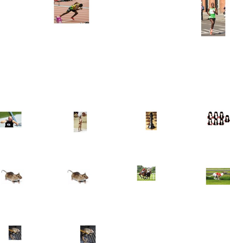
Figure 2. IMAP1 fitting in 17 events. Blue curves correspond to human systems (a–f), light purple one to
mouse (g,h), black one to the thoroughbred (i), brown one to greyhound (j), green one to the mouse lemur
(k,l). (a) Men sprint events, from the 100 m straight (blue dots) to the 3000 m (blue triangles) in T&F. (b) Men
long-distance running events, from the 5000 m (blue dots) to the marathon (blue triangles). (c) Is the shot put
(men), (d) is the clean & Jerk weight lifting (105+ kg, men), (e) is the chess event, (f) is the result from the
Cambridge face memory test event. (g,h) Are the weekly speed for male and female mice respectively. (i) Is the
speed of the thoroughbreds (1200 m turf competitions). (j) Is the greyhound speed in 480 m races (males &
females). (k,l) Are the grip strength for the male and female mouse lemurs respectively. Inset images in (a,c) are
licensed under the Creative Commons Attribution 2.0 Generic license (https://creativecommons.org/licenses/
by-sa/2.0/), inset image in (e) is licensed under the Creative Commons Attribution-Share Alike 2.5 Generic
license (https://creativecommons.org/licenses/by-sa/2.5/), inset images in (b,d,f,i–l) are licensed under the
Creative Commons Attribution-Share Alike 3.0 Unported license (https://creativecommons.org/licenses/by-
sa/3.0/) and inset images in (g,h) are in the public domain. Inset images are available at the following URLs:
(a) commons.wikimedia.org/wiki/File:London_2012_Yohan_Blake_200m_Q.jpg; (b) commons.wikimedia.
org/wiki/File:Patrick_Makau_Musyoki_running_world_record_at_Berlin_Marathon_2011.jpg; (c) commons.
wikimedia.org/wiki/File:Adam_Nelson_2010_Outdoors.jpg; (d) commons.wikimedia.org/wiki/File:RIAN_
archive_103479_Soviet_weight-lifter_Viktor_Mazin_during_the_XXII_Olympic_Games.jpg; (e) commons.
wikimedia.org/wiki/File:Chess_piece_-_Black_king.JPG; (f) commons.wikimedia.org/wiki/File:Universal_
emotions7.JPG; (g) commons.wikimedia.org/wiki/File:Mouse_white_background.jpg; (h) commons.
wikimedia.org/wiki/File:Mouse_white_background.jpg; (i) commons.wikimedia.org/wiki/File:Horse-racing-4.
jpg; (j) commons.wikimedia.org/wiki/File:Greyhound_Racing_4_amk.jpg; (k) commons.wikimedia.org/wiki/
File:Gray_Mouse_Lemur_1.JPG; (l) commons.wikimedia.org/wiki/File:Gray_Mouse_Lemur_1.JPG.
• The racing speeds of thoroughbreds were collected from international 1200 m on-turf competition over a
10-year period (2005–2014) (source: http://jra.jp/). A total of 1810 speeds were gathered.
SciEntific RepOrTS | (2019) 9:418 | DOI:10.1038/s41598-018-36707-3 5www.nature.com/scientificreports/
Figure 3. Normalized age of peak performance. It is computed as a percentage of estimated lifespan value:
peak /td.
Peak (year) Peak (year)
Time series R² (Moore) R² (IMAP1) Moore IMAP1
100 m (m.s−1) 0.9915 0.9924 25.88 24.99
400 m (m.s−1) 0.9819 0.9854 25.46 22.70
800 m (m.s−1) 0.9833 0.9848 25.74 25.40
3000 m (m.s−1) 0.9715 0.9742 23.53 28.24
5000 m (m.s−1) 0.9752 0.09815 25.65 28.95
10000 m (m.s−1) 0.9726 0.9803 25.74 30.15
Marathon (m.s−1) 0.9736 0.9764 27.82 26.94
Shotput (kg.m) 0.9174 0.9715 24.42 23.88
Weightlifting Clean & Jerk (kg) 0.9551 0.9757 24.72 31.39
Chess (score) 0.9781 0.9786 31.39 30.76
Facial recog. (proportion correct) 0.9501 0.9558 29.61 30.06
Greyhound (m.s−1) 0.9208 0.9207 23.31 22.18
Mouse males (km.week−1) 0.8801 0.8801 0.14 0.11
Mouse females (km.week−1) 0.9172 0.9163 0.15 0.15
Mouse lemur males (N) 0.0423 0.0330 1.53 3.59
Mouse lemur females (N) 0.0899 0.0843 4.87 × 10⁻² 2.06
Thoroughbred (m.s−1) 0.3981 0.3998 5.25 4.58
Table 1. Adjusted R² for both Eq. (1) (Moore) and Eq. (8) (IMAP1) along with the estimated age of peak
performance (year).
• Physical performance in greyhounds. A total of 26571 speeds (in m.s−1, for both males and females) were col-
lected from http://www.greyhound-data.com. The entire careers of the 100 best individuals of the 480 meters
(typical race distance) were gathered for each year over a ten-year period (2003–2012).
• The maximal distance per day in the wheel activity is recorded for mice (Mus domesticus) based on their vol-
untary behavior to practice wheel activity35. A total of 159 mice were genetically selected for high locomotor
activity and 14241 daily wheel running performances (7078 for males and 7163 for females) were gathered36.
The distance run was converted to km.week-1.
• The maximal grip strength of mouse lemurs (Microcebus murinus) was measured using a small iron bar
mounted on a piezo-electric force platform (Kistler squirrel force plate, ±0.1 N; Winterthur, Switzerland),
connected to a charge amplifier (Kistler charge amplifier type 9865). The pull strength was recorded during
60 s at 1 kHz. Animals performed the pull task several times during this interval. The task consisted of letting
the animal grab the iron bar and pull them horizontally until they let it go. The maximum force was then
extracted using the Bioware software (Kistler). The repeatability of this task was previously verified37. A sam-
ple of 359 individuals was measured: 170 females and 189 males, with 39 individuals tested twice. A total of
398 grip-strengths were measured.
The convex envelop was determined by gathering the top performance at each age in each time series. The
chosen time discretization is years of life for all traits measured in humans, months for traits measured in thor-
oughbreds and greyhounds, and weeks for traits measured in mice and mouse lemurs. All ages were converted to
years of life and speeds are converted in m.s−1, except for the mice in km.week−1. Both Eqs (1) and (8) were then
fit to each time series, including the two forces events, using a non-linear regression. The Levenberg-Marquardt
nonlinear least squares algorithm was used to provide the estimated parameters in both equations. It is a typi-
cal algorithm to solve non-linear least squares problems38. Typical goodness-of-fit indicators were estimated39
(Tables 1 and S3 and Supplementary Materials).
Credibility Interval (CI). A Monte-Carlo simulation was used to define a credibility interval in Eqs (1)
and (8). The estimated covariance matrix for the fitted parameters was estimated for each non-linear regres-
sion. A total of 100,000 new parameters were then drawn from a multi-dimensional normal distribution that
SciEntific RepOrTS | (2019) 9:418 | DOI:10.1038/s41598-018-36707-3 6www.nature.com/scientificreports/
uses this matrix. The two convex envelopes that contain all these iterations are presented for each equation (see
Supplementary Materials).
Time constants τ. In order to further investigate the biological scope of the model, we compared the time
constants τ provided by the model (1/αr) with the ones existing in the growth series. The primary assumption is
that the total number of cells N roughly corresponds to the body mass (kg) of the studied species. We collected
data from the official growth curves of the national French men population for humans and estimated the growth
curves from the mouse lemur cohort and a thoroughbred database (see Supplementary Materials, Table S4 and
Fig. S2).
Results
The age-related patterns are similar for the studied time series, revealing an inverted-U shape with continuous
transitions between development and senescence (Fig. 2). The IMAP1 model provides good estimates of the per-
formance on all time series (Fig. 2, Table 1, Supplementary Table S3). The normalization nevertheless reveals a
few differences (Table 2). Estimated coefficients differ widely in the strength series (shotput and weightlifting),
and in the mouse systems compared to other time series. They reveal a linear decline (small βr⁎ and high α 0⁎),
possibly related to missing data at advanced ages and/or small cohorts introducing large variability. The lack of
data during the steep decline is also quite important in the facial recognition time series, thus limiting the estima-
tion of td. In all studied systems, the age of peak performance occurs before the first half of the overall lifespan.
The average normalized value of the age of peak performance is: peak /t˜d where t̃d is the estimated age of death. The
peak performance is 20.49 ± 6.58% (Fig. 3).
Model comparison. Based on the previously defined goodness-of-fit indicators and the credibility interval,
the equation that best describes the age-performance relationship is the proposed one (Table 1 & S3 and Fig. S1):
mean R2 = 0.85 ± 0.29 (IMAP1) vs. 0.83 ± 0.28 (Moore) and mean RMSE = 2.54 ± 4.51 (IMAP1) vs. 3.79 ± 6.54
(Moore). The corrected Akaike information criterion shows that the model is the best candidate among the two,
except in 6 time series: greyhounds speed, both mouse lemur series and thoroughbred speed (Table S3). The
differences are small, putting forward a similar fit for the two equations in this series. The dynamic time warp-
ing distance shows that the two equations are close in almost all cases, except in the two force events (shotput
and weightlifting), chess rating and mice performance. Both equations do not suffer of over-parameterization
and suggest that second order polynomial and quadratic curve fitting will be less efficient in both describing
the age-performance relationship and providing an estimate of the age of peak performance. The CIs show that
the IMAP’s ones are narrower and converge as the age increase due to the explicit age of death parameter td. In
Moore’s equation, the CIs diverge as the age increases (Fig. S1), due to the lack of such a parameter.
Discussion
Aging research has widely focused on underlying mechanisms leading to observed declines in physical and phys-
iological capabilities. Many studies describe the decline in locomotor speed, perceptual or cognitive functions,
components of memory, reaction time, nerve conduction speed, muscular strength and flexibility, and other
traits, and show that experimental investigations are valuable because they provide information about the dynam-
ics of changes during the lifespan. In particular aging effects are studied in human sporting events9,11,12,22,25,40
where it is non-linear with time and has a declining curved shape. The extension of such research to other spe-
cies may also help in identifying the common physiological and biological features that are responsible for this
decline4,26. Other studies report a similar pattern while describing the decline in physical or physiological capac-
ities in mammals26, insects26 and even in some plants41. Thoroughbreds and greyhounds have historical records
in racing competitions. Data is very limited however: Racing horses are usually retired when they are 5 or 6 years
old (4 or 5 years old for greyhounds) because of health, attitude and performance issues.
The IMAP1 Eq. (8) is based on a coupled 2-phase approach of aging effects describing an increase in organ-
ism’s capabilities at younger ages and a global impairment at older ones. Two parameters are used to give possible
explanations in performance’s decline: the replicative senescence α(t) and the alteration in cellular effectiveness
β(t). The latter is related to a range of causes which are still under investigation. Possible candidates include
persistent metabolic waste products, interaction between damaged cell components (e.g., misfolded proteins),
reactive oxygen species, telomere attrition, etc42. Faced with the many theories proposed to explain aging -ranging
from the oxidative stress theory of aging to the antagonistic pleiotropy hypothesis43- we simply assume that the
cellular functionality experience cumulative stresses during aging.
Moore’s equation has been frequently used to describe changes in physical or cognitive performance with
aging10,25,27. A difference between Moore’s equation and the model presented herein is the additional parame-
ter td that corresponds to an explicit time of death, where the decreasing process reaches 0. The parameter td is
introduced in the IMAP1 and allows for both a controlled convergence and reduced variability near the time
of death (see the Monte-Carlo credibility interval analysis in the Supplementary Materials and Supplementary
Fig. S1). Moreover, the results show that estimated td are good approximations of empirical lifespan in each spe-
cies (Table 2). Although a minor correction in the model, it remains an important formalization step as it is
coupled to the developmental phase. The model can be adjusted to other physiological traits or species using any
typical statistical software that implements non-linear regression algorithms. The results provided in Table S1 can
also be useful to set the initial conditions of the algorithms (i.e. the initial values of the 4 parameters).
The IMAP1 allows for an accurate description of the studied physiological and physical events (Tables 1 and
2, Fig. 2 and Supplementary Table S3). While the physiological and biological processes implicated in those
time series may widely differ, they all exhibit a similar pattern. It also shows that the convex envelop of top
SciEntific RepOrTS | (2019) 9:418 | DOI:10.1038/s41598-018-36707-3 7www.nature.com/scientificreports/
Time series α 0⁎ α r⁎ βr⁎ td (year) 1/αr (year) τ (year)
100 m (m.s−1) 34.26 21.40 2.19 124.13 5.80 2.07, 9.21, 2.17 (*)
400 m (m.s−1) 67.64 25.51 2.79 109.54 4.29 /
800 m (m.s−1) 25.29 16.92 2.18 110.01 6.50 /
3000 m (m.s−1) 62.50 22.00 1.45 114.20 5.19 /
5000 m (m.s−1) 45.24 19.25 2.20 109.51 5.69 /
10000 m (m.s−1) 54.46 20.96 3.24 104.27 4.98 /
Marathon (m.s-1) 34.32 16.00 2.27 106.39 6.65 /
Shotput (kg.m) 223.84 20.28 3.01 × 10⁻⁴ 96.73 4.77 /
Weightlifting Clean & Jerk (kg) 1011.39 25.70 3.74 × 10⁻⁴ 95.96 3.73 /
Chess (score) 32.31 23.61 5.10 127.54 5.40 /
Facial recog. (proportion correct) 22.37 25.09 2.36 185.00 7.37 /
Greyhound (m.s−1) 77.83 39.96 5.64 11.37 0.28 N/A
Mouse males (km.week−1) 402.31 159.20 1.91 2.55 1.60 × 10⁻² [0.19, 0.25] (*)
Mouse females (km.week ) −1
108.53 83.74 0.97 2.53 3.02 × 10⁻² [0.37, 0.67] (*)
Mouse lemur males (N) 0.66 0.39 2.03 13.31 33.88 2.24
Mouse lemur females (N) 5.01 25.80 5.57 11.84 0.46 2.24
Thoroughbred (m.s−1) 1125.04 46.33 9.16 18.21 0.39 1.06
Table 2. Estimated parameters of Eq. (8), including td, αr and the estimated time constant τ for humans, mice,
mouse lemurs, greyhounds and thoroughbreds. Note. N/A = Not Available; (*) see Supplementary Materials
and Table S4 for details.
performances per age is congruent in different species, complementary to a previous work by Marck et al.26. The
estimated time constants are in the same order of magnitude as the ones estimated for growth curves, with a
few exceptions, of which mice are the most notable example (Table 2 and Supplementary Materials). It suggests
that the model can to some extent describe the link between cellular proliferation and performance dynamics,
despite its overall simplicity. It also strengthens the performance-body mass relationship in the developmental
stage, where an increase in mass leads to an increase in speed to a certain extent. The observed discrepancy in
mice would suggest that the impact of body mass on voluntary wheel-running activity is limited; however, several
important factors need to be considered. First, body mass was a strong predictor of voluntary wheel running in
the original selection experiments44. Second, body mass showed a negative correlated response to selection on
voluntary wheel running, indicating a negative genetic covariance between voluntary activity and body35. Third,
the mouse data presented here are from a population that experienced 16 generations of directional selection
for high voluntary wheel running activity, meaning these mice are genetically different from the original source
population of “normal” lab mice35. Nonetheless voluntary wheel-running activity may be weakly correlated
with maximum speed, as it may rely on other mechanisms that explain the difference, such as motivation and
coordination26,44.
The age of peak performance occurs at early ages (Fig. 3, Table 1) and all patterns exhibit a positive, right
skewed profile (Fig. 2). It suggests that the senescent phase is longer than the developmental one. In the model,
the detrimental processes start at the very initial stage of life but are compensated by the rapid growth of the
organism in size (Eq. (5)). The initial locomotor capabilities of most terrestrial species at the earlier ages tend to
be limited but not null: horse or zebra foals begin to walk anywhere from 45 minutes to 120 minutes after birth
and wildebeest can stand up and move a few minutes after birth45. Slight differences appear when looking at the
parameters (Table 2): both male and female mice have a higher αr⁎ than the other time series. It is known that
female mice mature earlier than males but display a later peak of activity than males46. Accordingly, the estimated
ages of peak activity are 8.1 weeks (females) and 5.9 weeks (males).
Complex changes in structure and function occur at all levels of biological organization, from cells to whole
body systems, eventually leading to the performance drop in a cumulative fashion47–49. This fits with previous
observations in which the decline in physical performance with aging was described as highly non-linear12,26. It
appears that maintaining a constant capacity at advanced ages is impossible and would require more and more
energy. The mice and strength series have a smaller βr⁎ than most other species, revealing a linear decline. This
may be related to a lack of or difficulties in implementing efficient exogenous artificial strategies (i.e., medical
interventions) that delay aging effects. Such strategies exist in human-related systems, including greyhounds and
thoroughbreds, where modern medical knowledge plus technological innovations slow the detrimental effects of
aging on performance. From a broader view, it would suggest that the inverted-U shape pattern and βr⁎ values are
related to the primary energy input50: the more energy is used to slow the decline, the higher βr⁎, although such an
idea has yet to be investigated. But this could explain why the resulting patterns have a more parabolic declining
shape in systems subject to medical intervention. The two strength events also present a linear decline, suggesting
that it is difficult to offset strength loss with age, contrary to traits such as distance running. The amount of data at
the extremes of aging is crucial, especially in organisms that exhibit a sharp pattern of growth toward maturity or
a sharp decline toward death. In the first case, the developmental stage is very brief so that it is difficult to gather
sufficient amounts of experimental data. The initial shape of the pattern is vague and this can lead to crude esti-
mates of the age of peak performance and αr. The mouse and mouse lemur are particularly affected by this issue.
SciEntific RepOrTS | (2019) 9:418 | DOI:10.1038/s41598-018-36707-3 8www.nature.com/scientificreports/
Likewise, the lack of data in the declining part of the lifespan can lead to flawed estimates of βr. This is the case in
the human facial recognition time series where it results in a widely overestimated td of 185 years old, which also
leads to an inconsistent normalized estimate in the age of peak performance (i.e. 16.25% of estimated lifespan for
a peak age of 30.06 years old). Correcting the value of td to td = 122 years old -the official maximum lifespan value
ever recorded- in Eq. (8), does not dramatically change the age of peak performance (i.e. 30.63 years old) but
produces a more normalized age of peak performance: 25.11%.
Conclusion
A common inverted-U pattern is found for a range of physiological traits in different species. As compared with
previous approaches, the proposed model accurately describes the age-related changes across the lifespan and is
based on an enhanced biological foundation. The approach provides consistent credibility intervals, in favor of a
finite lifespan with a non-linear decline of top performances at advanced ages. Additional investigations, targeting
an accurate measurement of both parameters αr, βr, should allow for integrating endogenous biological stresses
that increase with aging, such as extra-metabolic energy (i.e. independent of the calories derived from food
resources only) and environmental factors that may alter declining strength. However, beside its approximation
of the complex nature of the phenomenon, the IMAP1 provides a reasonable estimate of the age-performance
relationship. In addition, in the future the model can be made more sophisticated, such as including cell speciali-
zation and explicit cell renewal which could possibly increase the model’s biological accuracy and lead to a better
estimate of late-age performance decline.
References
1. Berthelot, G. et al. Has athletic performance reached its peak? Sports Med. 45, 1263–1271 (2015).
2. Tanaka, H. & Seals, D. R. Invited review: dynamic exercise performance in masters athletes: insight into the effects of primary
human aging on physiological functional capacity. J. Appl. Physiol. 95, 2152–2162 (2003).
3. Hill, A. V. The physiological basis of athletic records. Sci. Mon. 21, 409–428 (1925).
4. Justice, J. N., Cesari, M., Seals, D. R., Shively, C. A. & Carter, C. S. Comparative approaches to understanding the relation between
aging and physical function. J. Gerontol. Ser. Biomed. Sci. Med. Sci. 71, 1243–1253 (2015).
5. Desgorces, F.-D. et al. Similar slow down in running speed progression in species under human pressure. J. Evol. Biol. 25, 1792–1799
(2012).
6. Denny, M. W. Limits to running speed in dogs, horses and humans. J. Exp. Biol. 211, 3836–3849 (2008).
7. MacArthur, D. G. & North, K. N. Genes and human elite athletic performance. Hum. Genet. 116, 331–339 (2005).
8. Bouchard, C. et al. Familial aggregation of V o 2 max response to exercise training: results from the HERITAGE Family Study. J.
Appl. Physiol. 87, 1003–1008 (1999).
9. Allen, S. V. & Hopkins, W. G. Age of peak competitive performance of elite athletes: a systematic review. Sports Med. 45, 1431–1441
(2015).
10. Berthelot, G. et al. Exponential growth combined with exponential decline explains lifetime performance evolution in individual
and human species. Age 34, 1001–1009 (2012).
11. Tanaka, H. & Seals, D. R. Endurance exercise performance in Masters athletes: age‐associated changes and underlying physiological
mechanisms. J. Physiol. 586, 55–63 (2008).
12. Baker, A. B. & Tang, Y. Q. Aging performance for masters records in athletics, swimming, rowing, cycling, triathlon, and
weightlifting. Exp. Aging Res. 36, 453–477 (2010).
13. Ilmarinen, J. E. Aging workers. Occup. Environ. Med. 58, 546–546 (2001).
14. Böttiger, L. E. Regular decline in physical working capacity with age. Br Med J 3, 270–271 (1973).
15. Germine, L. T., Duchaine, B. & Nakayama, K. Where cognitive development and aging meet: Face learning ability peaks after age 30.
Cognition 118, 201–210 (2011).
16. Boot, A. M. et al. Peak bone mineral density, lean body mass and fractures. Bone 46, 336–341 (2010).
17. Kühnert, B. & Nieschlag, E. Reproductive functions of the ageing male. Hum. Reprod. Update 10, 327–339 (2004).
18. Salthouse, T. A. When does age-related cognitive decline begin? Neurobiol. Aging 30, 507–514 (2009).
19. Schoenberg, J. B., Beck, G. J. & Bouhuys, A. Growth and decay of pulmonary function in healthy blacks and whites. Respir. Physiol.
33, 367–393 (1978).
20. Knechtle, B., Rüst, C. A., Rosemann, T. & Lepers, R. Age-related changes in 100-km ultra-marathon running performance. Age 34,
1033–1045 (2012).
21. Knechtle, B., Valeri, F., Zingg, M. A., Rosemann, T. & Rüst, C. A. What is the age for the fastest ultra-marathon performance in time-
limited races from 6 h to 10 days? Age 36, 9715 (2014).
22. Baker, A. B., Tang, Y. Q. & Turner, M. J. Percentage Decline in Masters Superathlete Track and Field Performance With Aging. Exp.
Aging Res. 29, 47–65 (2003).
23. Maharam, L. G., Bauman, P. A., Kalman, D., Skolnik, H. & Perle, S. M. Masters Athletes: Factors Affecting Performance. Sports Med.
28, 273–285 (1999).
24. Belsky, D. W. et al. Quantification of biological aging in young adults. Proc. Natl. Acad. Sci. 112, E4104–E4110 (2015).
25. Guillaume, M. et al. Success and Decline: Top 10 Tennis Players follow a Biphasic Course. Med. Sci. Sports Exerc. 43, 2148–2154
(2011).
26. Marck, A. et al. Age-Related Changes in Locomotor Performance Reveal a Similar Pattern for Caenorhabditis elegans, Mus
domesticus, Canis familiaris, Equus caballus, and Homo sapiens. J. Gerontol. A. Biol. Sci. Med. Sci. glw136, https://doi.org/10.1093/
gerona/glw136 (2016)
27. Moore, D. H. A study of age group track and field records to relate age and running speed. Nature 253, 264–265 (1975).
28. Siler, W. A Competing-Risk Model for Animal Mortality. Ecology 60, 750–757 (1979).
29. Heligman, L. & Pollard, J. H. The age pattern of mortality. J. Inst. Actuar. 107, 49–80 (1980).
30. Hayward, A. D. et al. Asynchrony of senescence among phenotypic traits in a wild mammal population. Exp. Gerontol. 71, 56–68
(2015).
31. Lui, J. C. & Baron, J. Mechanisms Limiting Body Growth in Mammals. Endocr. Rev. 32, 422–440 (2011).
32. Lindner, A. B. & Demarez, A. Protein aggregation as a paradigm of aging. Biochim. Biophys. Acta BBA - Gen. Subj. 1790, 980–996
(2009).
33. Terman, A. & Brunk, U. T. Lipofuscin. Int. J. Biochem. Cell Biol. 36, 1400–1404 (2004).
34. Marquardt, D. W. An Algorithm for Least-Squares Estimation of Nonlinear Parameters. J. Soc. Ind. Appl. Math. 11, 431–441 (1963).
35. Morgan, T. J., Garland, T. & Carter, P. A. Ontogenies in mice selected for high voluntary wheel-running activity. I. Mean ontogenies.
Evolution 57, 646 (2003).
SciEntific RepOrTS | (2019) 9:418 | DOI:10.1038/s41598-018-36707-3 9www.nature.com/scientificreports/
36. Bronikowski, A. M., Morgan, T. J., Garland, T. & Carter, P. A. The evolution of aging and age-related physical decline in mice
selectively bred for high voluntary exercise. Evolution 60, 1494 (2006).
37. Thomas, P., Pouydebat, E., Brazidec, M. L., Aujard, F. & Herrel, A. Determinants of pull strength in captive grey mouse lemurs. J.
Zool. 298, 77–81 (2016).
38. Moré, J. J. The Levenberg-Marquardt algorithm: Implementation and theory. In Numerical Analysis (ed. Watson, G. A.) 105–116
(Springer Berlin Heidelberg, 1978).
39. Model Selection and Multimodel Inference. https://doi.org/10.1007/b97636 (Springer New York, 2004).
40. Schulz, R. & Curnow, C. Peak Performance and Age Among Superathletes: Track and Field, Swimming, Baseball, Tennis, and Golf.
J. Gerontol. 43, P113–P120 (1988).
41. Kasemsap, P, Crozat, Y & Satakhun, D. Cotton leaf photosynthesis and age relationship is influenced by leaf position. Nat Sci 31,
83–92.
42. López-Otín, C., Blasco, M. A., Partridge, L., Serrano, M. & Kroemer, G. The Hallmarks of Aging. Cell 153, 1194–1217 (2013).
43. Kirkwood, T. B. L. Understanding the Odd Science of Aging. Cell 120, 437–447 (2005).
44. Swallow, J. G., Carter, P. A. & Garland, T. Artificial Selection for Increased Wheel-Running Behavior in House Mice. Behav. Genet.
28, 227–237 (1998).
45. Estes, R. D. & Estes, R. K. The Birth and Survival of Wildebeest Calves. Z. Für Tierpsychol. 50, 45–95 (2010).
46. De MagalhãEs, J. P. & Costa, J. A database of vertebrate longevity records and their relation to other life-history traits. J. Evol. Biol.
22, 1770–1774 (2009).
47. West, G. B. & Bergman, A. Toward a Systems Biology Framework for Understanding Aging and Health Span. J. Gerontol. A. Biol. Sci.
Med. Sci. 64A, 205–208 (2009).
48. Zierer, J., Menni, C., Kastenmüller, G. & Spector, T. D. Integration of ‘omics’ data in aging research: from biomarkers to systems
biology. Aging Cell 14, 933–944 (2015).
49. Kriete, A., Sokhansanj, B. A., Coppock, D. L. & West, G. B. Systems approaches to the networks of aging. Ageing Res. Rev. 5, 434–448
(2006).
50. Smith, K. R. et al. Energy and Human Health. Annu. Rev. Public Health 34, 159–188 (2013).
Acknowledgements
This work was partially supported by the ‘Dynamique du Vieillir program’. We also are grateful to Burt Staniar and
Anne M. Bronikowski for their help and support regarding the thoroughbred and mice data respectively. Finally,
we are grateful to Jean-Michel Gaillard for his many helpful comments and suggestions.
Author Contributions
G.B., A.B.H., J.M.D.M. and J.F.T. conceived the study and designed methodology; G.B., P.N., P.A.C., A.M., V.F.,
P.B.Z.T., Js.S.A.J. conducted fieldwork and collected the data; G.B., J.M.D.M., S.D. and V.F. analyzed the data; G.B.,
A.M., P.A.C., J.M.D.M. and J.F.T. led the writing of the manuscript. All authors contributed critically to the drafts
and gave final approval for publication.
Additional Information
Supplementary information accompanies this paper at https://doi.org/10.1038/s41598-018-36707-3.
Competing Interests: The authors declare no competing interests.
Publisher’s note: Springer Nature remains neutral with regard to jurisdictional claims in published maps and
institutional affiliations.
Open Access This article is licensed under a Creative Commons Attribution 4.0 International
License, which permits use, sharing, adaptation, distribution and reproduction in any medium or
format, as long as you give appropriate credit to the original author(s) and the source, provide a link to the Cre-
ative Commons license, and indicate if changes were made. The images or other third party material in this
article are included in the article’s Creative Commons license, unless indicated otherwise in a credit line to the
material. If material is not included in the article’s Creative Commons license and your intended use is not per-
mitted by statutory regulation or exceeds the permitted use, you will need to obtain permission directly from the
copyright holder. To view a copy of this license, visit http://creativecommons.org/licenses/by/4.0/.
© The Author(s) 2019
SciEntific RepOrTS | (2019) 9:418 | DOI:10.1038/s41598-018-36707-3 10You can also read