And Partitionability into Senses - Let's Play Mono-Poly: BERT Can Reveal Words' Polysemy Level
←
→
Page content transcription
If your browser does not render page correctly, please read the page content below
Let’s Play Mono-Poly: BERT Can Reveal Words’ Polysemy Level
                                                              and Partitionability into Senses
                                                             Aina Garí Soler                           Marianna Apidianaki
                                                          Université Paris-Saclay                  Department of Digital Humanities
                                                              CNRS, LISN                                University of Helsinki
                                                           91400, Orsay, France                           Helsinki, Finland
                                                         aina.gari@limsi.fr                    marianna.apidianaki@helsinki.fi

                                                               Abstract

                                              Pre-trained language models (LMs) encode
                                              rich information about linguistic structure
                                              but their knowledge about lexical polysemy
arXiv:2104.14694v1 [cs.CL] 29 Apr 2021

                                              remains unclear. We propose a novel ex-
                                              perimental setup for analysing this knowl-
                                              edge in LMs specifically trained for dif-
                                              ferent languages (English, French, Span-
                                              ish and Greek) and in multilingual BERT.
                                              We perform our analysis on datasets care-
                                              fully designed to reflect different sense dis-
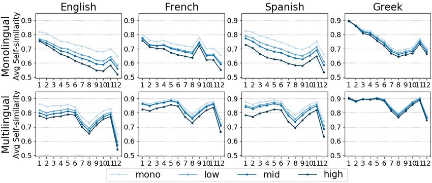
                                              tributions, and control for parameters that         Figure 1: BERT distinguishes monosemous (mono)
                                              are highly correlated with polysemy such as         from polysemous (poly) words in all layers. Rep-
                                              frequency and grammatical category. We              resentations for a poly word are obtained from
                                              demonstrate that BERT-derived represen-             sentences reflecting up to ten different senses
                                              tations reflect words’ polysemy level and           (poly-bal), the same sense (poly-same), or nat-
                                              their partitionability into senses. Polysemy-       ural occurrence in a corpus (poly-rand).
                                              related information is more clearly present
                                              in English BERT embeddings, but mod-
                                              els in other languages also manage to es-
                                                                                                  and Liang, 2019). The first probing tasks address-
                                              tablish relevant distinctions between words
                                              at different polysemy levels. Our results           ing semantic knowledge explored phenomena in
                                              contribute to a better understanding of the         the syntax-semantics interface, such as semantic
                                              knowledge encoded in contextualised rep-            role labelling and coreference (Tenney et al., 2019;
                                              resentations and open up new avenues for            Kovaleva et al., 2019), and the symbolic reason-
                                              multilingual lexical semantics research.            ing potential of LM representations (Talmor et al.,
                                                                                                  2020).
                                         1   Introduction                                            Lexical meaning was largely overlooked in
                                                                                                  early interpretation work, but is now attracting in-
                                         Pre-trained contextual language models have ad-          creasing attention. Pre-trained LMs have been
                                         vanced the state of the art in numerous natural          shown to successfully leverage sense annotated
                                         language understanding tasks (Devlin et al., 2019;       data for disambiguation (Wiedemann et al., 2019;
                                         Peters et al., 2018). Their success has motivated        Reif et al., 2019). The interplay between word
                                         a large number of studies exploring what these           type and token-level information in the hidden
                                         models actually learn about language (Voita et al.,      representations of LSTM LMs has also been ex-
                                         2019a; Clark et al., 2019; Voita et al., 2019b; Ten-     plored (Aina et al., 2019), as well as the simi-
                                         ney et al., 2019). The bulk of this interpretation       larity estimates that can be drawn from contextu-
                                         work relies on probing tasks which serve to predict      alised representations without directly addressing
                                         linguistic properties from the representations gen-      word meaning (Ethayarajh, 2019). In recent work,
                                         erated by the models (Linzen, 2018; Rogers et al.,       Vulić et al. (2020) probe BERT representations for
                                         2020). The focus was initially put on linguistic as-     lexical semantics, addressing out-of-context word
                                         pects pertaining to grammar and syntax (Linzen           similarity. Whether these models encode knowl-
                                         et al., 2016; Hewitt and Manning, 2019; Hewitt           edge about lexical polysemy and sense distinc-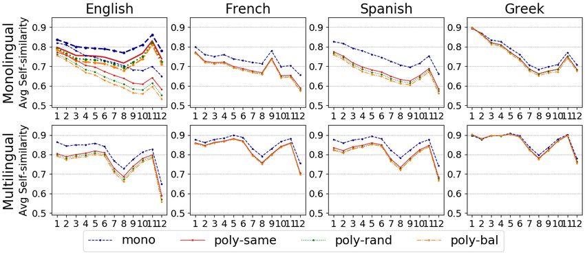
tions is, however, still an open question. Our work   to be present in a resource, and plan the time and
aims to fill this gap.                                effort needed in semantic annotation tasks (Mc-
   We propose methodology for exploring the           Carthy et al., 2016). It could also guide cross-
knowledge about word senses in contextualised         lingual transfer, serving to identify polysemous
representations. Our approach follows a rigorous      words for which transfer might be harder. Finally,
experimental protocol proper to lexical semantic      analysing words’ semantic space can be highly
analysis, which involves the use of datasets care-    useful for the study of lexical semantic change
fully designed to reflect different sense distribu-   (Rosenfeld and Erk, 2018; Dubossarsky et al.,
tions. This allows us to investigate the knowledge    2019; Giulianelli et al., 2020; Schlechtweg et al.,
models acquire during training, and the influence     2020). We make our code and datasets available to
of context variation on token representations. We     enable comparison across studies and to promote
account for the strong correlation between word       further research in these directions.1
frequency and number of senses (Zipf, 1945), and
for the relationship between grammatical category
                                                      2   Related Work
and polysemy, by balancing the frequency and part     The knowledge pre-trained contextual LMs en-
of speech (PoS) distributions in our datasets and     code about lexical semantics has only recently
applying a frequency-based model to polysemy          started being explored. Works by Reif et al. (2019)
prediction.                                           and Wiedemann et al. (2019) propose experiments
   Importantly, our investigation encompasses         using representations built from Wikipedia and the
monolingual models in different languages (En-        SemCor corpus (Miller et al., 1993), and show that
glish, French, Spanish and Greek) and multilin-       BERT can organise word usages in the semantic
gual BERT (mBERT). We demonstrate that BERT           space in a way that reflects the meaning distinc-
contextualised representations encode an impres-      tions present in the data. It is also shown that
sive amount of knowledge about polysemy, and          BERT can perform well in the word sense dis-
are able to distinguish monosemous (mono) from        ambiguation (WSD) task by leveraging the sense-
polysemous (poly) words in a variety of set-          related information available in these resources.
tings and configurations (cf. Figure 1). Impor-       These works address the disambiguation capabili-
tantly, we demonstrate that representations de-       ties of the model but do not show what BERT ac-
rived from contextual LMs encode knowledge            tually knows about words’ polysemy, which is the
about words’ polysemy acquired through pre-           main axis of our work. In our experiments, sense
training which is combined with information           annotations are not used to guide the models into
from new contexts of use (Sections 3-6). Addi-        establishing sense distinctions, but rather for cre-
tionally, we show that BERT representations can       ating controlled conditions that allow us to analyse
serve to determine how easy it is to partition a      BERT’s inherent knowledge of lexical polysemy.
word’s semantic space into senses (Section 7).           Probing has also been proposed for lexical se-
   Our methodology can serve for the analy-           mantics analysis, but addressing different ques-
sis of words and datasets from different top-         tions than the ones posed in our work. Aina et al.
ics, domains and languages. Knowledge about           (2019) probe the hidden representations of a bidi-
words’ polysemy and sense partitionability has        rectional (bi-LSTM) LM for lexical (type-level)
numerous practical implications: it can guide         and contextual (token-level) information. They
decisions towards a sense clustering or a per-        specifically train diagnostic classifiers on the tasks
instance approach in applications (Reisinger          of retrieving the input embedding of a word and
and Mooney, 2010; Neelakantan et al., 2014;           a representation of its contextual meaning (as re-
Camacho-Collados and Pilehvar, 2018); point to        flected in its lexical substitutes). The results show
words with stable semantics which can be safe         that the information about the input word that is
cues for disambiguation in running text (Lea-         present in LSTM representations is not lost after
cock et al., 1998; Agirre and Martinez, 2004;         contextualisation; however, the quality of the in-
Loureiro and Camacho-Collados, 2020); deter-          formation available for a word is assessed through
mine the needs in terms of context size for dis-      the model’s ability to identify the corresponding
ambiguation (e.g. in queries, chatbots); help lexi-     1
                                                          Our code and data are available at https://github.
cographers define the number of entries for a word    com/ainagari/monopoly.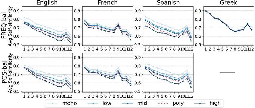
Setting          Word        Sense              Sentences
                                INN                The walk ended, inevitably, right in front of his hotel building.
   mono             hotel.n
                                INN                Maybe he’s at the hotel.
                                CHAMBER            The room vibrated as if a giant hand had rocked it.
   poly-same room.n
                                CHAMBER            (...) Tell her to come to Adam’s room (...)
                                CHAMBER            (...) he left the room, walked down the hall (...)
   poly-bal         room.n      SPACE              It gives them room to play and plenty of fresh air.
                                OPPORTUNITY        Even here there is room for some variation, for metal surfaces vary (...)

             Table 1: Example sentences for the monosemous noun hotel and the polysemous noun room.

embedding, as in Adi et al. (2017) and Conneau                     tations, which amounts to word usage similarity
et al. (2018). Also, lexical ambiguity is only                     (Usim) estimation, a classical task in lexical se-
viewed through the lens of contextualisation. In                   mantics (Erk et al., 2009; Huang et al., 2012; Erk
our work, on the contrary, it is given a central                   et al., 2013). The Usim task precisely involves
role: we explicitly address the knowledge BERT                     predicting the similarity of word instances in con-
encodes about words’ degree of polysemy and par-                   text without use of sense annotations. BERT has
titionability into senses. Vulić et al. (2020) also               been shown to be particularly good at this task
propose to probe contextualised models for lexi-                   (Garí Soler et al., 2019; Pilehvar and Camacho-
cal semantics, but they do so using “static” word                  Collados, 2019). Our experiments allow to ex-
embeddings obtained through pooling over several                   plore and understand what this ability is due to.
contexts, or extracting representations for words in
isolation and from BERT’s embedding layer, be-                     3       Lexical Polysemy Detection
fore contextualisation. These representations are                  3.1      Dataset Creation
evaluated on tasks traditionally used for assessing
the quality of static embeddings, such as out-of-                  We build our English dataset using SemCor 3.0
context similarity and word analogy, which are not                 (Miller et al., 1993), a corpus manually annotated
tailored for addressing lexical polysemy. Other                    with WordNet senses (Fellbaum, 1998). It is im-
contemporaneous work explores lexical polysemy                     portant to note that we do not use the annotations
in static embeddings (Jakubowski et al., 2020),                    for training or evaluating any of the models. These
and the relation of ambiguity and context uncer-                   only serve to control the composition of the sen-
tainty as approximated in the space constructed by                 tence pools that are used for generating contextu-
mBERT using information-theoretic measures (Pi-                    alised representations, and to analyse the results.
mentel et al., 2020). Finally, work by Ethayarajh                  We form sentence pools for monosemous (mono)
(2019) provides useful observations regarding the                  and polysemous (poly) words that occur at least
impact of context on the representations, without                  ten times in SemCor.3 For each mono word, we
explicitly addressing the semantic knowledge en-                   randomly sample ten of its instances in the cor-
coded by the models. Through an exploration of                     pus. For each poly word, we form three sentence
BERT, ELMo and GPT-2 (Radford et al., 2019),                       pools of size ten reflecting different sense distribu-
the author highlights the highly distorted similar-                tions:
ity of the obtained contextualised representations
                                                                       • Balanced (poly-bal). We sample a sen-
which is due to the anisotropy of the vector space
                                                                         tence for each sense of the word in SemCor
built by each model.2 The question of meaning is
                                                                         until a pool of ten sentences is formed.
not addressed in this work, making it hard to draw
any conclusions about lexical polysemy.                                • Random (poly-rand). We randomly sam-
    Our proposed experimental setup is aimed at                          ple ten poly word instances from SemCor.
investigating the polysemy information encoded                           We expect this pool to be highly biased to-
in the representations built at different layers of                      wards a specific sense due to the skewed fre-
deep pre-trained LMs. Our approach basically re-                         quency distribution of word senses (Kilgar-
lies on the similarity of contextualised represen-                       riff, 2004; McCarthy et al., 2004). This con-
   2                                                                   3
    This issue affects all tested models and is particularly            We find the number of senses for a word of a specific part
present in the last layers of GPT-2, resulting in highly similar   of speech (PoS) in WordNet 3.0, which we access through the
representations even for random words.                             NLTK interface (Bird et al., 2009).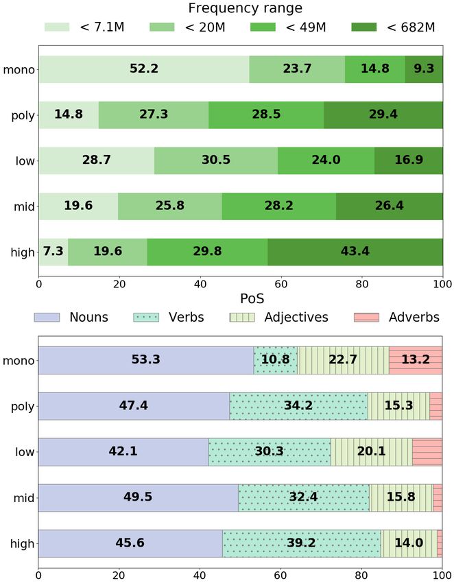
figuration is closer to the expected natural oc-           2019)9 , ELMo (Peters et al., 2018) and con-
       currence of senses in a corpus, it thus serves             text2vec (Melamud et al., 2016). BERT is a
       to estimate the behaviour of the models in a               Transformer architecture (Vaswani et al., 2017)
       real-world setting.                                        that is jointly trained for a masked LM and
   • Same sense (poly-same). We sample ten                        a next sentence prediction task. Masked LM
     sentences illustrating only one sense of the                 inolves a Cloze-style task, where the model
     poly word. Although the composition of                       needs to guess randomly masked words by
     this pool is similar to that of the mono pool                jointly conditioning on their left and right con-
     (i.e. all instances describe the same sense) we              text. We use the bert-base-uncased and
     call it poly-same because it describes one                   bert-base-cased models, pre-trained on the
     sense of a polysemous word.4 Specifically,                   BooksCorpus (Zhu et al., 2015) and English
     we want to explore whether BERT represen-                    Wikipedia. ELMo is a bi-LSTM LM trained
     tations derived from these instances can serve               on Wikipedia and news crawl data from WMT
     to distinguish mono from poly words.                         2008-2012. We use 1024-d representations from
                                                                  the 5.5B model.10       Context2vec is a neural
The controlled composition of the poly sentence                   model based on word2vec’s CBOW architecture
pools allows us to investigate the behaviour of the               (Mikolov et al., 2013) which learns embeddings
models when they are exposed to instances of pol-                 of wide sentential contexts using a bi-LSTM. The
ysemous words describing the same or different                    model produces representations for words and
senses. There are 1,765 poly words in Sem-                        their context. We use the context representations
Cor with at least 10 sentences available.5 We                     from a 600-d context2vec model pre-trained on the
randomly subsample 418 from these in order to                     ukWaC corpus (Baroni et al., 2009).11
balance the mono and poly classes. Our En-                           For French, Spanish and Greek, we use BERT
glish dataset is composed of 836 mono and poly                    models specifically trained for each language:
words, and their instances in 8,195 unique sen-                   Flaubert (flaubert_base_uncased) (Le
tences. Table 1 shows a sample of the sentences                   et al., 2020), BETO (bert-base-spanish-
in different pools. For French, Spanish and Greek,                wwm-uncased) (Cañete et al., 2020), and Greek
we retrieve sentences from the Eurosense corpus                   BERT (bert-base-greek-uncased-v1)
(Delli Bovi et al., 2017) which contains texts from               (Koutsikakis et al., 2020). We also use the
Europarl automatically annotated with BabelNet                    bert-base-multilingual-cased model
word senses (Navigli and Ponzetto, 2012).6 We                     for each of the four languages. mBERT was
extract sentences from the high precision version7                trained on Wikipedia data of 104 languages.12 All
of Eurosense, and create sentence pools in the                    BERT models generate 768-d representations.
same way as in English, balancing the number of
monosemous and polysemous words (418). We                         3.3    The Self-Similarity Metric
determine the number of senses for a word as the                  All models produce representations that describe
number of its Babelnet senses that are mapped to                  word meaning in specific contexts of use. For each
a WordNet sense.8                                                 instance i of a target word w in a sentence, we
3.2    Contextualised Word Representations                        extract its representation from: (i) each of the 12
                                                                  layers of a BERT model;13 (ii) each of the three
We experiment with representations generated
                                                                     9
by three English models: BERT (Devlin et al.,                           We use Huggingface transformers (Wolf et al.,
                                                                  2020).
   4                                                                 10
     The polysemous words are the same as in poly-bal                   https://allennlp.org/elmo
                                                                     11
and poly-rand.                                                          https://github.com/orenmel/
   5
     We use sentences of up to 100 words.                         context2vec
   6                                                                 12
     BabelNet is a multilingual semantic network built from             The mBERT model developers recommend us-
multiple lexicographic and encyclopedic resources, such as        ing the cased version of the model rather than the
WordNet and Wikipedia.                                            uncased one, especially for languages with non-
   7
     The high coverage version of Eurosense is larger than the    Latin alphabets, because it fixes normalisation issues.
high precision one, but disambiguation is less accurate.          More details about this model can be found here:
   8
     This filtering serves to exclude BabelNet senses that cor-   https://github.com/google-research/bert/
respond to named entities and are not useful for our purposes     blob/master/multilingual.md.
                                                                     13
(such as movie or album titles), and to run these experiments           We also tried different combinations of the last four lay-
under similar conditions across languages.                        ers, but this did not improve the results. When a word is split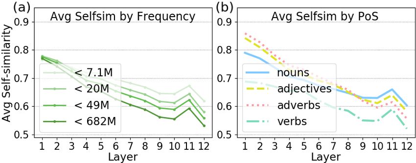
ELMo layers; (iii) context2vec. We calculate self-             poly-same pools, which contain instances of
similarity (Self Sim) (Ethayarajh, 2019) for w in              only one sense. This distinction is important; it
a sentence pool p and a layer l, by taking the aver-           suggests that BERT encodes information about
age of the pairwise cosine similarities of the rep-            a word’s monosemous or polysemous nature re-
resentations of its instances in l:                            gardless of the sentences that are used to derive
                        1    XX                                the contextualised representations. Specifically,
Self Siml (w) = 2                    cos(xwli , xwlj )         BERT produces less similar representations for
                    |I| −|I|
                                i∈I j∈I                        word instances in the poly-same pool compared
                                    j6=i
                                                 (1)           to mono, reflecting that poly words can have dif-
In formula 1, |I| is the number of instances for w             ferent meanings.
(ten in our experiments); xwli and xwlj are the rep-              We also observe a clear ordering of the three
resentations for instances i and j of w in layer l.            poly sentence pools: average Self Sim is higher
The Self Sim score is in the range [-1, 1]. We re-             in poly-same, which only contains instances
port the average Self Sim for all w’s in a pool p.             of one sense, followed by mid-range values in
We expect it to be higher for monosemous words                 poly-rand, and gets its lowest values in the bal-
and words with low polysemy than for highly pol-               anced setting (poly-bal). This is noteworthy
ysemous words. We also expect the poly-same                    given that poly-rand contains a mix of senses
pool to have a higher average Self Sim score than              but with a stronger representation of w’s most fre-
the other poly pools which contain instances of                quent sense than poly-bal (71% vs. 47%).14
different senses.                                                 Our results demonstrate that BERT representa-
   Contextualisation has a strong impact on                    tions encode two types of lexical semantic knowl-
Self Sim since it introduces variation in the                  edge: information about the polysemous na-
token-level representations, making them more                  ture of words acquired through pre-training (as
dissimilar. The Self Sim value for a word would                reflected in the distinction between mono and
be 1 with non-contextualised (or static) embed-                poly-same), and information from the partic-
dings, as all its instances would be assigned the              ular instances of a word used to create the con-
same vector. In contextual models, Self Sim is                 textualised representations (as shown by the finer-
lower in layers where the impact of the context is             grained distinctions between different poly set-
stronger (Ethayarajh, 2019). It is, however, impor-            tings). BERT’s knowledge about polysemy can be
tant to note that contextualisation in BERT models             due to differences in the types of context where
is not monotonic, as shown by previous studies of              words of different polysemy levels occur. We ex-
the models’ internal workings (Voita et al., 2019a;            pect poly words to be seen in more varied con-
Ethayarajh, 2019). Our experiments presented in                texts than mono words, reflecting their different
the next section provide additional evidence in this           senses. BERT encodes this variation with the
respect.                                                       LM objective through exposure to large amounts
                                                               of data, and this is reflected in the representa-
3.4   Results and Discussion                                   tions. The same ordering pattern is observed
3.4.1 Mono-Poly in English                                     with mBERT (lower part of Figure 2) and with
                                                               ELMo (Figure 3 (a)). With context2vec, average
Figure 2 shows the average Self Sim value ob-                  Self Sim in mono is 0.40, 0.38 in poly-same,
tained for each sentence pool with representations             0.37 in poly-rand, and 0.35 in poly-bal.
produced by BERT models. The thin lines in                     This suggests that these models also have some in-
the first plot illustrate the average Self Sim score           herent knowledge about lexical polysemy, but dif-
calculated for mono and poly words using rep-                  ferences are less clearly marked than in BERT.
resentations from each layer of the uncased En-
                                                                  Using the cased model leads to an overall in-
glish BERT model. We observe a clear distinction
                                                               crease in Self Sim and to smaller differences be-
of words according to their polysemy: Self Sim
                                                               tween bands, as shown by the thick lines in the first
is higher for mono than for poly words across
                                                               plot of Figure 2. Our explanation for the lower
all layers and sentence pools. BERT establishes
                                                               distinction ability of the bert-base-cased
a clear distinction even between the mono and
                                                               model is that it encodes sparser information about
into multiple wordpieces (WPs), we obtain its representation
                                                                 14
by averaging the WPs.                                                 Numbers are macro-averages for words in the pools.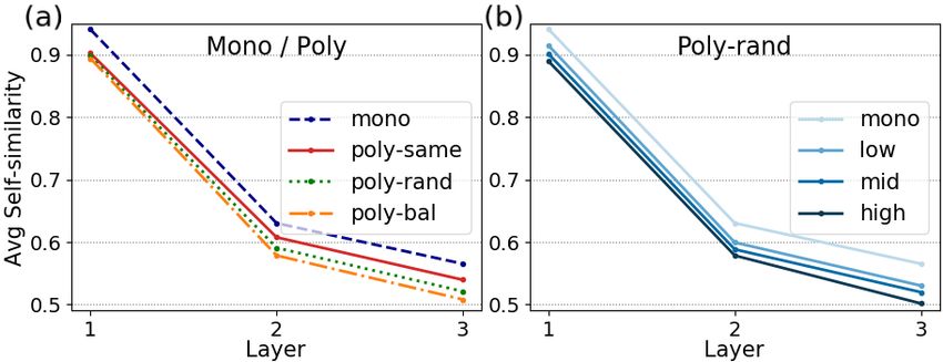
Figure 2: Average Self Sim obtained with monolingual BERT models (top row) and mBERT (bottom row) across
all layers (horizontal axis). In the first plot, thick lines correspond to the cased model.

                                                            The decreasing trend in Self Sim observed for
                                                         BERT in Figure 2, and the peak in layer 11, con-
                                                         firm the phases of context encoding and token re-
                                                         construction observed by Voita et al. (2019a).15 In
                                                         earlier layers, context variation makes representa-
                                                         tions more dissimilar and Self Sim decreases. In
                                                         the last layers, information about the input token is
Figure 3: Comparison of average Self Sim obtained        recovered for LM prediction and similarity scores
for mono and poly words using ELMo representa-           are boosted. Our results show clear distinctions
tions (a), and for words in different polysemy bands     across all BERT and ELMo layers. This suggests
in the poly-rand sentence pool (b).                      that lexical information is spread throughout the
                                                         layers of the models, and contributes new evidence
words than the uncased model. It was trained             to the discussion on the localisation of semantic
on a more diverse set of strings, so many WPs            information inside the models (Rogers et al., 2020;
are present in both their capitalised and non-           Vulić et al., 2020).
capitalised form in the vocabulary. In spite of that,
                                                         3.4.2 Mono-Poly in Other Languages
it has a smaller vocabulary size (29K WPs) than
the uncased model (30.5K). Also, a higher num-           The top row of Figure 2 shows the average
ber of WPs correspond to word parts than in the          Self Sim obtained for French, Spanish and Greek
uncased model (6,478 vs 5,829).                          words using monolingual models.            Flaubert,
   We test the statistical significance of the           BETO and Greek BERT representations clearly
mono/poly-rand distinction using unpaired                distinguish mono and poly words, but average
two-samples t-tests when the normality assump-           Self Sim values for different poly pools are
tion is met (as determined with Shapiro Wilk’s           much closer than in English. BETO seems to
tests). Otherwise, we run a Mann Whitney U               capture these fine-grained distinctions slightly bet-
test, the non-parametrical alternative of this t-test.   ter than the French and Greek models. The sec-
In order to lower the probability of type I errors       ond row of the Figure shows results obtained with
(false positives) that increases when performing         mBERT representations. We observe the highly
multiple tests, we correct p-values using the Ben-       similar average Self Sim values assigned to dif-
jamini–Hochberg False Discovery Rate (FDR) ad-           ferent poly pools, which show that distinction is
justment (Benjamini and Hochberg, 1995). Our             harder than in monolingual models.
results show that differences are significant across       15
                                                              They study the information flow in the Transformer esti-
all embedding types and layers (α = 0.01).               mating the MI between representations at different layers.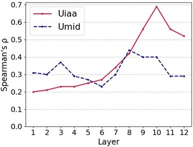
Figure 4: Average Self Sim obtained with monolingual BERT models (top row) and mBERT (bottom row)
for mono and poly words in different polysemy bands. Representations are derived from sentences in the
poly-rand pool.

                                                                 6, high: k > 6. For English, the three bands
                                                                 are populated with a different number of words:
                                                                 low: 551, mid: 663, high: 551. In the other
                                                                 languages, we form bands containing 300 words
                                                                 each.17 In Figure 4, we compare mono words with
                                                                 words in each polysemy band in terms of their av-
                                                                 erage Self Sim. Values for mono words are taken
Figure 5: Comparison of BERT average Self Sim for                from Section 3. For poly words, we use rep-
mono and poly words in different polysemy bands in               resentations from the poly-rand sentence pool
the poly-bal and poly-same sentence pools.                       which better approximates natural occurrence in a
                                                                 corpus. For comparison, we report in Figure 5 re-
   Statistical tests show that the difference                    sults obtained in English using sentences from the
between Self Sim values in mono and                              poly-same and poly-bal pools.18
poly-rand is significant in all layers of                           In English, the pattern is clear in all plots:
BETO, Flaubert, Greek BERT, and mBERT for                        Self Sim is higher for mono than for poly words
Spanish and French.16 The magnitude of the                       in any band, confirming that BERT is able to dis-
difference in Greek BERT is, however, smaller                    tinguish mono from poly words at different pol-
compared to the other models (0.03 vs. 0.09 in                   ysemy levels. The range of Self Sim values for
BETO at the layers with the biggest difference in                a band is inversely proportional to its k: words in
average Self Sim).                                               low get higher values than words in high. The
                                                                 results denote that the meaning of highly poly-
4    Polysemy Level Prediction                                   semous words is more variable (lower Self Sim)
                                                                 than the meaning of words with fewer senses. As
4.1 SelfSim-based Ranking                                        expected, scores are higher and inter-band simi-
In this set of experiments, we explore the impact                larities are closer in poly-same (cf. Figure 5
of words’ degree of polysemy on the representa-                  (b)) compared to poly-rand and poly-bal,
tions. We control for this factor by grouping words              where distinctions are clearer. The observed dif-
into three polysemy bands as in McCarthy et al.                  ferences confirm that BERT can predict the pol-
(2016), which correspond to a specific number of
senses (k): low: 2 ≤ k ≤ 3, mid: 4 ≤ k ≤                           17
                                                                       We only used 418 of these poly words in Section 3 in
                                                                 order to have balanced mono and poly pools.
   16                                                               18
      In mBERT for Greek, the difference is significant in ten         We omit the plots for poly-bal and poly-same for
layers.                                                          the other models due to space constraints.
be explained to some extent by the quality of
the automatic EuroSense annotations, which has
a direct impact on the quality of the sentence
pools. Results of a manual evaluation conducted
by Delli Bovi et al. (2017) showed that WSD pre-
cision is ten points higher in English (81.5) and
Spanish (82.5) than in French (71.8). The Greek
portion, however, has not been evaluated.
Plots in the second row of Figure 4 show re-
sults obtained using mBERT. Similarly to the pre-
vious experiment (Section 3.4), mBERT overall
makes less clear distinctions than the monolin-
gual models. The low and mid bands often
get similar Self Sim values, which are close to
mono in French and Greek. Still, inter-band dif-
ferences are significant in most layers of mBERT
and the monolingual French, Spanish and Greek
models.21
4.2 Anisotropy Analysis
In order to better understand the reasons behind
the smaller inter-band differences observed with
mBERT, we conduct an additional analysis of
the models’ anisotropy. We create 2,183 random
word pairs from the English mono, low, mid
Figure 6: The left plots show the similarity between
and high bands, and 1,318 pairs in each of the
random words in models for each language. Plots on
the right side show the difference between the similar- other languages.22 We calculate the cosine simi-
ity of random words and Self Sim in poly-rand. larity between two random instances of the words
in each pair and take the average over all pairs
(RandSim). The plots in the left column of
ysemy level of words, even from instances de- Figure 6 show the results. We observe a clear
scribing the same sense. difference in the scores obtained by monolingual
We observe similar patterns with ELMo (cf. models (solid lines) and mBERT (dashed lines).
Figure 3 (b)) and context2vec representations in Clearly, mBERT assigns higher similarities to ran-
poly-rand,19 but smaller absolute inter-band dom words, an indication that its semantic space
differences. In poly-same, both models fail is more anisotropic than the one built by mono-
to correctly order the bands. Overall, our re- lingual models. High anisotropy means that rep-
sults highlight that BERT encodes higher qual- resentations occupy a narrow cone in the vector
ity knowledge about polysemy. We test the sig- space, which results in lower quality similarity es-
nificance of the inter-band differences detected in timates and in the model’s limited potential to es-
poly-rand using the same approach as in Sec- tablish clear semantic distinctions.
tion 3.4.1. These are significant in all but a few20 We also compare RandSim to the aver-
layers of the models. age Self Sim obtained for poly words in the
The bands are also correctly ranked in the other poly-rand sentence pool (cf. Section 3.1).
three languages but with smaller inter-band differ- In a quality semantic space, we would expect
ences than in English, especially in Greek where Self Sim (between same word instances) to be
clear distinctions are only made in a few mid- much higher than RandSim. The right column of
dle layers. This variation across languages can Figure 6 shows the difference between these two
19 21
Average Self Sim values for context2vec in the With the exception of mono→low in mBERT for
poly-rand setting: low: 0.37, mid: 0.36, high: 0.36. Greek, and low→mid in Flaubert and in mBERT for French.
20 22
low→mid in ELMo’s third layer, and mid→high in 1,318 is the total number of words across bands in
context2vec and in BERT’s first layer. French, Spanish and Greek.Figure 8: Average Self Sim for English words of dif-
ferent frequencies and part of speech categories with
BERT representations.
5.1 Dataset Composition
We perform this analysis in English using fre-
quency information from Google Ngrams (Brants
and Franz, 2006). For French, Spanish and Greek,
we use frequency counts gathered from the OS-
CAR corpus (Suárez et al., 2019). We split the
words into four ranges (F ) corresponding to the
quartiles of frequencies in each dataset. Each
range f in F contains the same number of words.
We provide detailed information about the com-
Figure 7: Composition of the English word bands in position of the English dataset in Figure 7.23 Fig-
terms of frequency (a) and grammatical category (b). ure 7(a) shows that mono words are much less
frequent than poly words. Figure 7(b) shows
scores. diff in a layer l is calculated as in Equa- the distribution of different PoS categories in each
tion 2: band. Nouns are the prevalent category in all
bands and verbs are less present among mono
diffl = Avg Self Siml (poly−rand) − RandSiml words (10.8%), as expected. Finally, adverbs are
(2) hardly represented in the high polysemy band
We observe that the difference is smaller in the (1.2% of all words).
space built by mBERT, which is more anisotropic
than the space built by monolingual models. This 5.2 Self-Sim by Frequency Range and PoS
is particularly obvious in the upper layers of the We examine the average BERT Self Sim per fre-
model. This result confirms the lower quality of quency range in poly-rand. Due to space con-
mBERT’s semantic space compared to monolin- straints, we only report detailed results for the En-
gual models. glish BERT model in Figure 8 (plot (a)). The
Finally, we believe that another factor behind clear ordering by range suggests that BERT can
the worse mBERT performance is that the multi- successfully distinguish words by their frequency,
lingual WP vocabulary is mostly English-driven, especially in the last layers. Plot (b) in Figure 8
resulting in arbitrary partitionings of words in the shows the average Self Sim for words of each
other languages. This word splitting procedure PoS category. Verbs have the lowest Self Sim
must have an impact on the quality of the lexical which is not surprising given that they are highly
information in mBERT representations. polysemous (as shown in Figure 7(b)). We ob-
serve the same trend for monolingual models in
5 Analysis by Frequency and PoS the other three languages.
Given the strong correlation between word fre-
5.3 Controlling for Frequency and PoS
quency and number of senses (Zipf, 1945), we
explore the impact of frequency on BERT repre- We conduct an additional experiment where we
sentations. Our goal is to determine the extent to control for the composition of the poly bands
which it influences the good mono/poly detec- 23
The composition of each band is the same as in Sections
tion results obtained in Sections 3.4 and 4.1. 3 and 4.Figure 9: Average Self Sim inside the poly bands balanced for frequency (FREQ-bal) and part of speech (POS-
bal). Self Sim is calculated using representations generated by monolingual BERT models from sentences in each
language-specific pool. We do not balance the Greek dataset for PoS because it only contains nouns.
in terms of grammatical category and word fre-
POS -bal
quency. We call these two settings POS-bal and
Nouns Verbs Adjectives Adverbs
FREQ -bal. We define npos , the smallest number
en 198 45 64 7
of words of a specific PoS that can be found in a
fr 171 32 29 9
band. We form the POS-bal bands by subsampling es 167 22 40 0
from each band the same number of words (npos )
of that PoS. For example, all POS-bal bands have FREQ -bal
nn nouns and nv verbs. We follow a similar pro-
en 7.1M 20M 49M 682M
cedure to balance the bands by frequency in the 40 99 62 39
FREQ -bal setting. In this case, nf is the minimum 23m 70m 210m 41M
fr
number of words of a specific frequency range f 17 43 67 38
that can be found in a band. We form the FREQ-bal es 64m 233m 793m 59M
dataset by subsampling from each band the same 12 39 58 48
number of words (nf ) of a given range f in F . el 14m 40m 111m 1.9M
13 41 70 42
Table 2 shows the distribution of words per PoS
and frequency range in the POS-bal and FREQ- Table 2: Content of the polysemy bands in the POS-
bal settings for each language. The table reads bal and FREQ-bal settings. All bands for a language
as follows: the English POS-bal bands contain contain the same number of words of a specific gram-
198 nouns, 45 verbs, 64 adjectives and 7 adverbs; matical category or frequency range. M stands for a
similarly for the other two languages. Greek is million and m for a thousand occurrences of a word in
not included in this POS-based analysis because a corpus.
all sense-annotated Greek words in EuroSense are
nouns. In FREQ-bal, each English band con- or part of speech. The only exception is Greek
tains 40 words that occur less than 7.1M times in BERT which cannot establish correct inter-band
Google Ngrams, and so on and so forth. distinctions when the influence of frequency is
We examine the average Self Sim values ob- neutralised in the FREQ-bal setting. A general ob-
tained for words in each band in poly-rand. servation that applies to all models is that although
Figure 9 shows the results for monolingual mod- inter-band distinctions become less clear, the or-
els. We observe that the mono and poly words dering of the bands is preserved. We observe the
in the POS-bal and FREQ-bal bands are ranked same trend with ELMo and context2vec.
similarly to Figure 4. This shows that BERT’s Statistical tests show that all inter-band distinc-
polysemy predictions do not rely on frequency tions established by English BERT are still signif-icant in most layers of the model.24 This is not the mono/poly poly bands
case for ELMo and context2vec, which can dis- Model Self Sim pairCos Self Sim pairCos
BERT 0.7610 0.798 0.4910 0.4610
tinguish between mono and poly words but fail mBERT 0.778 0.758 0.4612 0.4312
to establish significant distinctions between poly-
EN
ELMo 0.692 0.633 0.372 0.343
semy bands in the balanced settings. For French context2vec 0.61 0.61 0.34 0.31
and Spanish, the statistical analysis shows that all Frequency 0.77 0.41
distinctions in POS-bal are significant in at least Flaubert 0.587 0.556 0.298 0.279
FR
one layer of the models. The same applies to the mBERT 0.669 0.649 0.387 0.388
Frequency 0.61 0.37
mono→poly distinction in FREQ-bal but finer- BETO 0.709 0.667 0.426 0.485
grained distinctions disappear.25
ES
mBERT 0.6911 0.647 0.389 0.437
Frequency 0.67 0.41
6 Classification by Polysemy Level GreekBERT 0.704 0.644 0.344 0.386
EL
mBERT 0.607 0.657 0.3211 0.349
Our finding that word instance similarity differs Frequency 0.63 0.35
across polysemy bands suggests that this feature Baseline 0.50 0.25
can be useful for classification. In this Sec-
Table 3: Accuracy of binary (mono/poly) and multi-
tion, we probe the representations for polysemy class (poly bands) classifiers using Self Sim and
using a classification experiment where we test pairCos features on the test sets. Comparison to a
their ability to guess whether a word is polyse- baseline that predicts always the same class and a clas-
mous, and which poly band it falls in. We use sifier that only uses log frequency as feature. Subscripts
the poly-rand sentence pools and a standard denote the layers used.
train/dev/test split (70/15/15%) of the data. For the
mono/poly distinction (i.e. the data used in Sec- Table 3 presents classification accuracy on the
tion 3), this results in 584/126/126 words per set test set. We report results obtained with the best
in each language. To guarantee a fair evaluation, layer for each representation type and feature as
we make sure there is no overlap between the lem- determined on the development sets. In English,
mas in the three sets. We use two types of features: best accuracy is obtained by BERT in both the
(i) the average Self Sim for a word; (ii) all pair- binary (0.79) and multiclass settings (0.49), fol-
wise cosine similarities collected for its instances, lowed by mBERT (0.77 and 0.46). Despite its sim-
which results in 45 features per word (pairCos). plicity, the frequency-based classifier obtains bet-
We train a binary logistic regression classifier for ter results than context2vec and ELMo, and per-
each type of representation and feature. forms on par with mBERT in the binary setting.
As explained in Section 4, the three poly bands This shows that frequency information is highly
(low, mid and high) and mono contain a dif- relevant for the mono-poly distinction. All clas-
ferent number of words. For classification into sifiers outperform the same class baseline. These
polysemy bands, we balance each class by ran- results are very encouraging, showing that BERT
domly subsampling words from each band. In embeddings can be used to determine whether a
total, we use 1,168 words for training, 252 for word has multiple meanings, and provide a rough
development and 252 for testing (70/15/15%) in indication of its polysemy level. Results in the
English. In the other languages, we use a split other three languages are not as high as those ob-
of 840/180/180 words. We train multi-class lo- tained in English, but most models give higher re-
gistic regression classifiers with the two types of sults than the frequency-based classifier.26
features, Self Sim and pairCos. We compare
the results of the classifiers to a baseline that pre- 7 Word Sense Clusterability
dicts always the same class, and to a frequency-
based classifier which only uses the words’ log We have shown that representations from pre-
frequency in Google Ngrams, or in the OSCAR trained LMs encode rich information about words’
corpus, as a feature. degree of polysemy. They can successfully distin-
guish mono from poly lemmas, and predict the
24
Note that the sample size in this analysis is smaller com- polysemy level of words. Our previous experi-
pared to that used in Sections 3.4 and 4.1.
25 26
With a few exceptions: mono→low and mid→high Only exceptions are Greek mBERT in the multi-class
are significant in all BETO layers. setting, and Flaubert in both settings.ments involved a set of controlled settings repre- tations generated by BERT, context2vec and
senting different sense distributions and polysemy ELMo (BERT-REP, c2v-REP, ELMo-REP);27 us-
levels. In this Section, we explore whether these ing substitute-based representations with auto-
representations can also point to the clusterability matically generated substitutes. The substitute-
of poly words in an uncontrolled setting. based approach allows for a direct comparison
with the method of McCarthy et al. (2016). They
7.1 Task Definition represent each instance i of a word w in Usim as
Instances of some poly words are easier to group a vector ~i, where each substitute s assigned to w
into interpretable clusters than others. This is, for over all its instances (i ∈ I) becomes a dimen-
example, a simple task for the ambiguous noun sion (ds ). For a given i, the value for each ds
rock which can express two clearly separate senses is the number of annotators who proposed substi-
(STONE and MUSIC), but harder for book which tute s. ds contains a zero entry if s was not pro-
might refer to the CONTENT or OBJECT senses of posed for i. We refer to this type of representa-
the word (e.g. I read a book vs. I bought a book). tion as Gold-SUB. We generate our substitute-
In what follows, we test the ability of contextu- based representations with BERT using the simple
alised representations to estimate how easy this “word similarity” approach in Zhou et al. (2019).
task is for a specific word, i.e. its partitionability For an instance i of word w in context C, we rank
into senses. a set of candidate substitutes S = {s1 , s2 , ..., sn }
Following McCarthy et al. (2016), we use the based on the cosine similarity of the BERT repre-
clusterability metrics proposed by Ackerman and sentations for i and for each substitute sj ∈ S in
Ben-David (2009) to measure the ease of clus- the same context C. We use representations from
tering word instances into senses. McCarthy et the last layer of the model. As candidate substi-
al. base their clustering on the similarity of man- tutes, we use the unigram paraphrases of w in the
ual meaning-preserving annotations (lexical sub- Paraphrase Database (PPDB) XXL package (Gan-
stitutes and translations). Instances of different itkevitch et al., 2013; Pavlick et al., 2015).28
senses, such as: Put granola bars in a bowl vs. For each instance i of w, we obtain a ranking
That’s not a very high bar, present no overlap in R of all substitutes in S. We remove low-quality
their in-context substitutes: {snack, biscuit, block, substitutes (i.e. noisy paraphrases or substitutes
slab} vs. {pole, marker, hurdle, barrier, level, ob- referring to a different sense of w) using the filter-
struction}. Semantically related instances, on the ing approach proposed by Garí Soler et al. (2019).
contrary, share a different number of substitutes We check each pair of substitutes in subsequent
depending on their proximity. The need for man- positions in R, starting from the top; if a pair is
ual annotations, however, constrains the method’s unrelated in PPDB, all substitutes from that posi-
applicability to specific datasets. tion onwards are discarded. The idea is that good
We propose to extend and scale up the Mc- quality substitutes should be both high-ranked and
Carthy et al. (2016) clusterability approach using semantically related. We build vectors as in Mc-
contextualised representations, in order to make it Carthy et al. (2016), using the cosine similarity
applicable to a larger vocabulary. These experi- assigned by BERT to each substitute as a value.
ments are carried out in English due to the lack of We call this representation BERT-SUB.
evaluation data in other languages.
7.3 Sense Clustering
7.2 Data
The clusterability metrics that we use are met-
We run our experiments on the usage similarity rics initially proposed for estimating the quality of
(Usim) dataset (Erk et al., 2013) for comparison the optimal clustering that can be obtained from a
with previous work. Usim contains ten instances dataset; the better the quality of this clustering, the
for 56 target words of different PoS from the Se- higher the clusterability of the dataset it is derived
mEval Lexical Substitution dataset (McCarthy and
27
Navigli, 2007). Word instances are manually an- We do not use the first layer of ELMo in this experiment.
notated with pairwise similarity scores on a scale It is character-based, so most representations of a lemma are
identical and we cannot obtain meaningful clusters.
from 1 (completely different) to 5 (same meaning). 28
We use PPDB (http://www.paraphrase.org) to
We represent target word instances in Usim reduce variability in our substitute sets, compared to the ones
in two ways: using contextualised represen- that would be proposed by looking at the whole vocabulary.Gold Metric BERT-REP c2v-REP ELMo-REP BERT-SUB Gold-SUB BERT-AGG Gold-AGG
SEP & -0.48*10 -0.12 -0.242 -0.03 -0.20 -0.48*11 –
Uiaa VR % 0.1712 0.14 0.192 0.09 0.34* 0.33*12 –
SIL % 0.61*11 0.06 0.212 0.10 0.32* 0.69*10 0.80*
SEP % 0.43*9 -0.01 0.083 0.05 0.16 0.43*9 –
Umid VR & -0.249 -0.08 -0.153 -0.15 -0.24 -0.32*5 –
SIL & -0.46*10 0.05 -0.062 -0.11 -0.38* -0.44*8 -0.48*
Table 4: Spearman’s ρ correlation between automatic metrics and gold standard clusterability estimates. Significant
correlations (where the null hypothesis ρ = 0 is rejected with α < 0.05) are marked with *. The arrows indicate
the expected direction of correlation for each metric. Subscripts indicate the layer that achieved best performance.
The two strongest correlations obtained with each gold standard measure are in boldface.
from (Ackerman and Ben-David, 2009). k clusters and its range is [0,1). We use k-means’
In order to estimate the clusterability of a word sum of squared distances of data points to their
w, we thus need to first cluster its instances in the closest cluster center as the loss. Details about
data. We use the k-means algorithm which re- these two metrics are given in Appendix A.30 We
quires the number of senses for a lemma. This is, also experiment with SIL as a clusterability met-
of course, different for every lemma in our dataset. ric, as it can assess cluster validity. For VR and
We define the optimal number of clusters k for a SIL, a higher value indicates higher clusterability.
lemma in a data-driven manner using the Silhou- The inverse applies to SEP.
ette coefficient (SIL) (Rousseeuw, 1987), without We calculate Spearman’s ρ correlation between
recourse to external resources.29 For a data point the results of each clusterability metric and two
i, SIL compares the intra-cluster distance (i.e. the gold standard measures derived from Usim: Uiaa
average distance from i to every other data point and Umid. Uiaa is the inter-annotator agreement
in the same cluster) with the average distance of for a lemma in terms of average pairwise Spear-
i to all points in its nearest cluster. The SIL value man’s correlation between annotators’ judgments.
for a clustering is obtained by averaging SIL for all Higher Uiaa values indicate higher clusterability,
data points, and it ranges from -1 to 1. We cluster meaning that sense partitions are clearer and eas-
each type of representation for w using k-means ier to agree upon. Umid is the proportion of mid-
with a range of k values (2 ≤ k ≤ 10), and re- range judgments (between 2 and 4) assigned by
tain the k of the clustering with the highest mean annotators to all instances of a target word. It in-
SIL . Additionally, since BERT representations’ dicates how often usages do not have identical (5)
cosine similarity correlates well with usage simi- or completely different (1) meaning. Therefore,
larity (Garí Soler et al., 2019), we experiment with higher Umid values indicate lower clusterability.
Agglomerative Clustering with average linkage di-
rectly on the cosine distance matrix obtained with 7.5 Results and Discussion
BERT representations (BERT-AGG). For com- The clusterability results are given in Table 4. Ag-
parison, we also use Agglomerative Clustering on glomerative Clustering on the gold Usim simi-
the gold usage similarity scores from Usim, trans- larity scores (Gold-AGG) gives best results on
formed into distances (Gold-AGG). the Uiaa evaluation in combination with the SIL
clusterability metric (ρ = 0.80). This is unsur-
7.4 Clusterability Metrics prising, since Uiaa and Umid are derived from
We use in our experiments the two best perform- the same Usim scores. From our automatically
ing metrics from McCarthy et al. (2016): Variance generated representations, the strongest correla-
Ratio (VR) (Zhang, 2001) and Separability (SEP) tion with Uiaa (0.69) is obtained with BERT-AGG
(Ostrovsky et al., 2012). VR calculates the ratio and the SIL clusterability metric. The SIL met-
of the within- and between-cluster variance for a ric also works well with BERT-REP achieving the
given clustering solution. SEP measures the differ- strongest correlation with Umid (-0.46). It consti-
ence in loss between two clusterings with k−1 and 30
Note that the VR and SEP metrics are not compatible with
Gold-AGG which relies on Usim similarity scores, because
29
We do not use McCarthy et al.’s graph-based approach we need vectors for their calculation. For BERT-AGG, we
because it is not compatible with all our representation types. calculate VR and SEP using BERT embeddings.guages, as shown by our experiments on French,
Spanish and Greek, and to a lesser extent for mul-
tilingual BERT. Moreover, English BERT repre-
sentations can be used to obtain a good estimation
of a word’s partitionability into senses. These re-
sults open up new avenues for research in multilin-
gual semantic analysis, and we can consider vari-
ous theoretical and application-related extensions
for this work.
The polysemy and sense-related knowledge re-
Figure 10: Spearman’s ρ correlations between the gold
standard Uiaa and Umid scores, and clusterability es- vealed by the models can serve to develop novel
timates obtained using Agglomerative Clustering on a methodologies for improved cross-lingual align-
cosine distance matrix of BERT representations. ment of embedding spaces and cross-lingual trans-
fer, pointing to more polysemous (or less cluster-
able) words for which transfer might be harder.
tutes, thus, a good alternative to the SEP and VR
Predicting the polysemy level of words can also
metrics used in previous studies when combined
be useful for determining the context needed for
with BERT representations.
acquiring representations that properly reflect the
Interestingly, the correlations obtained using
meaning of word instances in running text. From
raw BERT contextualised representations are
a more theoretical standpoint, we expect this work
much higher than the ones observed with Mc-
to be useful for studies on the organisation of the
Carthy et al. (2016)’s representations which rely
semantic space in different languages and on lexi-
on manual substitutes (Gold-SUB). These were in
cal semantic change.
the range of 0.20-0.34 for Uiaa and 0.16-0.38 for
Umid (in absolute value). The results demonstrate Acknowledgements
that BERT representations offer good estimates
of the partitionability of words into senses, im- This work has been supported by the
proving over substitute annotations. As expected, French National Research Agency un-
the substitution-based approach performs better der project ANR-16-CE33-0013. The
with clean manual substitutes (Gold-SUB) than work is also part of the FoTran project,
with automatically generated ones (BERT-SUB). funded by the European Research
We present a per layer analysis of the corre- Council (ERC) under the European Union’s Hori-
lations obtained with the best performing BERT zon 2020 research and innovation programme
representations (BERT-AGG) and the SIL metric (grant agreement № 771113). We thank the anony-
in Figure 10. We report the absolute values of the mous reviewers and the TACL Action Editor for
correlation coefficient for a more straightforward their careful reading of our paper, their thorough
comparison. For Uiaa, the higher layers of the reviews and their helpful suggestions.
model make the best predictions: correlations in-
crease monotonically up to layer 10, and then they
References
show a slight decrease. Umid prediction shows a
more irregular pattern: it peaks at layers 3 and 8, Margareta Ackerman and Shai Ben-David. 2009.
and decreases again in the last layers. Clusterability: A Theoretical Study. Journal of
Machine Learning Research, 5:1–8.
8 Conclusion
Yossi Adi, Einat Kermany, Yonatan Belinkov, Ofer
We have shown that contextualised BERT repre- Lavi, and Yoav Goldberg. 2017. Fine-grained
sentations encode rich information about lexical Analysis of Sentence Embeddings Using Auxil-
polysemy. Our experimental results suggest that iary Prediction Tasks. In Proceedings of ICLR,
this high quality knowledge about words, which Toulon, France.
allows BERT to detect polysemy in different con-
figurations and across all layers, is acquired dur- Eneko Agirre and David Martinez. 2004. Un-
ing pre-training. Our findings hold for the English supervised WSD based on Automatically Re-
BERT as well as for BERT models in other lan- trieved Examples: The Importance of Bias. InProceedings of the 2004 Conference on Empir- Neural Networks for NLP, pages 276–286, Flo-
ical Methods in Natural Language Processing, rence, Italy. Association for Computational Lin-
pages 25–32, Barcelona, Spain. Association for guistics.
Computational Linguistics.
Alexis Conneau, German Kruszewski, Guillaume
Laura Aina, Kristina Gulordava, and Gemma Lample, Loïc Barrault, and Marco Baroni.
Boleda. 2019. Putting Words in Context: 2018. What you can cram into a single $&!#*
LSTM Language Models and Lexical Ambigu- vector: Probing sentence embeddings for lin-
ity. In Proceedings of the 57th Annual Meeting guistic properties. In Proceedings of the 56th
of the Association for Computational Linguis- Annual Meeting of the Association for Compu-
tics, pages 3342–3348, Florence, Italy. Associ- tational Linguistics (Volume 1: Long Papers),
ation for Computational Linguistics. pages 2126–2136, Melbourne, Australia. Asso-
ciation for Computational Linguistics.
Marco Baroni, Silvia Bernardini, Adriano Fer-
raresi, and Eros Zanchetta. 2009. The WaCky Claudio Delli Bovi, Jose Camacho-Collados,
Wide Web: a Collection of Very Large Linguis- Alessandro Raganato, and Roberto Navigli.
tically Processed Web-Crawled Corpora. Jour- 2017. EuroSense: Automatic Harvesting of
nal of Language Resources and Evaluation, Multilingual Sense Annotations from Parallel
43(3):209–226. Text. In Proceedings of the 55th Annual Meet-
ing of the Association for Computational Lin-
Yoav Benjamini and Yosef Hochberg. 1995. Con- guistics (Volume 2: Short Papers), pages 594–
trolling the False Discovery Rate: a Practical 600, Vancouver, Canada. Association for Com-
and Powerful Approach to Multiple Testing. putational Linguistics.
Journal of the Royal statistical society: series
B (Methodological), 57(1):289–300. Jacob Devlin, Ming-Wei Chang, Kenton Lee, and
Kristina Toutanova. 2019. BERT: Pre-training
Steven Bird, Ewan Klein, and Edward Loper.
of Deep Bidirectional Transformers for Lan-
2009. Natural Language Processing with
guage Understanding. In Proceedings of the
Python: Analyzing Text with the Natural Lan-
2019 Conference of the North American Chap-
guage Toolkit. O’Reilly Media, Inc., Beijing.
ter of the Association for Computational Lin-
Thorsten Brants and Alex Franz. 2006. Web 1T 5- guistics: Human Language Technologies, Vol-
gram Version 1. In LDC2006T13, Philadelphia, ume 1 (Long and Short Papers), pages 4171–
Pennsylvania. Linguistic Data Consortium. 4186, Minneapolis, Minnesota. Association for
Computational Linguistics.
José Camacho-Collados and Mohammad Taher
Pilehvar. 2018. From Word To Sense Embed- Haim Dubossarsky, Simon Hengchen, Nina Tah-
dings: A Survey on Vector Representations of masebi, and Dominik Schlechtweg. 2019.
Meaning. Journal of Artificial Intelligence Re- Time-Out: Temporal Referencing for Robust
search, 63:743–788. Modeling of Lexical Semantic Change. In Pro-
ceedings of the 57th Annual Meeting of the As-
José Cañete, Gabriel Chaperon, Rodrigo Fuentes, sociation for Computational Linguistics, pages
and Jorge Pérez. 2020. Spanish Pre-Trained 457–470, Florence, Italy. Association for Com-
BERT Model and Evaluation Data. In Proceed- putational Linguistics.
ings of the ICLR 2020 Workshop on Practical
ML for Developing Countries (PML4DC), Ad- Katrin Erk, Diana McCarthy, and Nicholas Gay-
dis Ababa, Ethiopia. lord. 2009. Investigations on Word Senses and
Word Usages. In Proceedings of the Joint Con-
Kevin Clark, Urvashi Khandelwal, Omer Levy, ference of the 47th Annual Meeting of the ACL
and Christopher D. Manning. 2019. What Does and the 4th International Joint Conference on
BERT Look at? An Analysis of BERT’s Atten- Natural Language Processing of the AFNLP,
tion. In Proceedings of the ACL 2019 Work- pages 10–18, Suntec, Singapore. Association
shop BlackboxNLP: Analyzing and Interpreting for Computational Linguistics.You can also read


