Exposing Semantic Segmentation Failures via Maximum Discrepancy Competition
←
→
Page content transcription
If your browser does not render page correctly, please read the page content below
Exposing Semantic Segmentation Failures via Maximum Discrepancy
                                        Competition
                                        Jiebin Yan 1 · Yu Zhong 1 · Yuming Fang 1 · Zhangyang Wang 2 · Kede Ma 3
arXiv:2103.00259v2 [cs.CV] 3 Mar 2021

                                        Abstract Semantic segmentation is an extensively studied              diagnosis of ten PASCAL VOC semantic segmentation al-
                                        task in computer vision, with numerous methods proposed               gorithms. With detailed analysis of experimental results, we
                                        every year. Thanks to the advent of deep learning in seman-           point out strengths and weaknesses of the competing algo-
                                        tic segmentation, the performance on existing benchmarks is           rithms, as well as potential research directions for further
                                        close to saturation. A natural question then arises: Does the         advancement in semantic segmentation. The codes are pub-
                                        superior performance on the closed (and frequently re-used)           licly available at https://github.com/QTJiebin/
                                        test sets transfer to the open visual world with unconstrained        MAD_Segmentation.
                                        variations? In this paper, we take steps toward answering the
                                                                                                              Keywords Semantic segmentation · Performance evalua-
                                        question by exposing failures of existing semantic segmen-
                                                                                                              tion · Generalization · Maximum discrepancy competition
                                        tation methods in the open visual world under the constraint
                                        of very limited human labeling effort. Inspired by previous
                                        research on model falsification, we start from an arbitrar-           1 Introduction
                                        ily large image set, and automatically sample a small im-
                                        age set by MAximizing the Discrepancy (MAD) between                   Deep learning techniques have been predominant in vari-
                                        two segmentation methods. The selected images have the                ous computer vision tasks, such as image classification (He
                                        greatest potential in falsifying either (or both) of the two          et al., 2016; Krizhevsky et al., 2012; Simonyan and Zisser-
                                        methods. We also explicitly enforce several conditions to di-         man, 2014), object detection (Ren et al., 2015), and seman-
                                        versify the exposed failures, corresponding to different un-          tic segmentation (Long et al., 2015). One important reason
                                        derlying root causes. A segmentation method, whose fail-              for the remarkable successes of deep learning techniques
                                        ures are more difficult to be exposed in the MAD compe-               is the establishment of large-scale human-labeled databases
                                        tition, is considered better. We conduct a thorough MAD               for different vision tasks. However, years of model develop-
                                                                                                              ment on the same benchmarks may raise the risk of overfit-
                                        Jiebin Yan                                                            ting due to excessive re-use of the test data. This poses a new
                                        E-mail: jiebinyan@foxmail.com
                                                                                                              challenge for performance comparison in computer vision:
                                        Yu Zhong
                                        E-mail: zhystu@qq.com                                                    How to probe the generalization of “top-performing”
                                        Yuming Fang (Corresponding Author)                                       computer vision methods (measured on closed and well-
                                        E-mail: fa0001ng@e.ntu.edu.sg                                            established test sets) to the open visual world with much
                                        Zhangyang Wang                                                           greater content variations?
                                        E-mail: atlaswang@utexas.edu
                                        Kede Ma                                                                   Here we focus our study on semantic segmentation,
                                        E-mail: kede.ma@cityu.edu.hk                                          which involves partitioning a digital image into semanti-
                                                                                                              cally meaningful segments, for two main reasons. First, pre-
                                        1 School of Information Technology, Jiangxi University of Fi-         vious studies on generalizability testing are mostly restricted
                                        nance and Economics, Nanchang, Jiangxi, China.
                                        2 Department of Electrical and Computer Engineering, The University
                                                                                                              to image classification (Goodfellow et al., 2014), while lit-
                                        of Texas at Austin, Austin, Texas, USA.                               tle attention has been received for semantic segmentation
                                        3 Department of Computer Science, City University of Hong Kong,       despite its close relationship to many high-stakes applica-
                                        Kowloon, Hong Kong.                                                   tions, such as self-driving cars and computer-aided diagno-
2                                                                                                                       Jiebin Yan 1 et al.

sis systems. Second, semantic segmentation requires pixel-                – An extensive demonstration of our method to diagnose
level dense labeling, which is a much more expensive and                    ten semantic segmentation methods on PASCAL VOC,
time-consuming endeavor compared to that of image clas-                     where we spot the generalization pitfalls of even the
sification and object detection. According to Everingham                    strongest segmentation method so far, pointing to poten-
et al. (2015), it can easily take ten times as long to segment              tial directions for improvement.
an object than to draw a bounding box around it, making
the human labeling budget even more unaffordable for this
particular task. As it is next to impossible to create a larger          2 Related Work
human-labeled image set as a closer approximation of the
open visual world, the previous question may be rephrased                In this section, we first give a detailed overview of semantic
in the context of semantic segmentation:                                 segmentation, with emphasis on several key modules that
        How to leverage massive unlabeled images from the                have been proven useful to boost performance on standard
        open visual world to test the generalizability of seman-         benchmarks. We then review emerging ideas to test different
        tic segmentation methods under a very limited human              aspects of model generalizability in computer vision.
        labeling budget?
     Inspired by previous studies on model falsification in
the field of computational neuroscience (Golan et al., 2019),            2.1 Semantic Segmentation
software testing (McKeeman, 1998), image processing (Ma
et al., 2020), and computer vision (Wang et al., 2020),                  Traditional methods (Cao and Fei-Fei, 2007; Csurka and
we take steps toward answering the question by efficiently               Perronnin, 2008; Shotton et al., 2008) relied exclusively on
exposing semantic segmentation failures using the MAxi-                  hand-crafted features such as textons (Julesz, 1981), his-
mum Discrepancy (MAD) competition1 (Wang et al., 2020).                  togram of oriented gradients (Dalal and Triggs, 2005), and
Specifically, given a web-scale unlabeled image set, we au-              bag-of-visual-words (Kadir and Brady, 2001; Lowe, 2004;
tomatically mine a small image set by maximizing the dis-                Russell et al., 2006), coupled with different machine learn-
crepancy between two semantic segmentation methods. The                  ing techniques, including random forests (Shotton et al.,
selected images are the most informative in terms of dis-                2008), support vector machines (Yang et al., 2012), and con-
criminating between two methods. Therefore, they have the                ditional random fields (Verbeek and Triggs, 2008). The per-
great potential to be the failures of at least one method. We            formance of these knowledge-driven methods is highly de-
also specify a few conditions to encourage spotting more                 pendent on the quality of the hand-crafted features, which
diverse failures, which may correspond to different under-               are bound to have limited expressive power. With the intro-
lying causes. We seek such small sets of images for every                duction of fully convolutional networks (Long et al., 2015),
distinct pair of the competing segmentation methods, and                 many existing semantic segmentation algorithms practiced
merge them into one, which we term as the MAD image                      end-to-end joint optimization of feature extraction, group-
set. Afterwards, we allocate the limited human labeling bud-             ing and classification, and obtained promising results on
get to the MAD set, sourcing the ground-truth segmentation               closed and well-established benchmarks. Here, we summa-
map for each selected image. Comparison of model predic-                 rize four key design choices of convolutional neural net-
tions and human labels on the MAD set strongly indicates                 works (CNNs) that significantly advance the state-of-the-art
the relative performance of the competing models. In this                of semantic segmentation.
case, a better segmentation method is the one with fewer                     1) Dilated Convolution (Yu and Koltun, 2015), also
failures exposed by other algorithms. We apply this gen-                 known as atrous convolution, is specifically designed for
eral model falsification method to state-of-the-art semantic             dense prediction. With an extra parameter to control the
segmentation methods trained on the popular benchmark of                 rate of dilation, it aggregates multi-scale context information
PASCAL VOC (Everingham et al., 2015). Analysis of the                    without sacrificing spatial resolution. However, dilated con-
resulting MAD set yields a number of insightful and previ-               volution comes with the so-called gridding problem. Wang
ously overlooked findings on the PASCAL VOC dataset.                     et al. (2018) proposed hybrid dilated convolution to effec-
     In summary, our contributions include:                              tively alleviate the gridding issue by gradually increasing the
    – A computational framework to efficiently expose diverse            dilation rates in each stage of convolutions. Yu et al. (2017)
      and even rare semantic segmentation failures based on              developed dilated residual networks for semantic segmenta-
      the MAD competition.                                               tion with max pooling removed. DeepLabv3+ (Chen et al.,
    1
                                                                         2018b), the latest version of the well-known DeepLab fam-
    Note that MAD is different from “Maximum Mean Discrepancy”
                                                                         ily (Chen et al., 2017, 2018a,b) combined dilated convolu-
(Tzeng et al., 2014). The former means maximizing the difference be-
tween the predictions of two test models, while the latter is a method   tion with spatial pyramid pooling for improved extraction of
of computing distances between probability distributions.                multi-scale contextual information.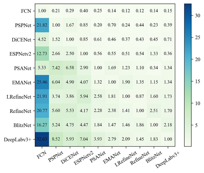
Exposing Semantic Segmentation Failures via Maximum Discrepancy Competition                                                    3

    2) Skip Connection. In the study of fully convolutional        the HVS, whose goal is to extract and leverage the most rel-
networks for semantic segmentation, Long et al. (2015)             evant information to the vision task at hand. Some studies
adopted skip connections to fuse low-level and high-level          attempted to advance semantic segmentation by incorporat-
information, which is helpful for generating sharper bound-        ing attention mechanism. Li et al. (2018) proposed a fea-
aries. U-Net (Ronneberger et al., 2015) and its variant (Zhou      ture pyramid attention module to combine attention mecha-
et al., 2018) used dense skip connections to combine fea-          nism with pyramid representation, resulting in more precise
ture maps of the encoder and the corresponding decoder,            dense prediction. Fu et al. (2019a) presented a self-attention
and achieved great successes in medical image segmen-              mechanism in semantic segmentation, which involves a po-
tation. SegNet (Badrinarayanan et al., 2017) implemented           sition attention module to aggregate important spatial fea-
a similar network architecture for semantic segmentation,          tures scattered across different locations, and a channel at-
and compensated for the reduced spatial resolution with            tention module to emphasize interdependent feature maps.
index-preserving max pooling. Fu et al. (2019b) proposed a         Zhao et al. (2018b) proposed a point-wise spatial attention
stacked deconvolutional network by stacking multiple small         network to aggregate long-range contextual information and
deconvolutional networks (also called “units”) for fine re-        to enable bi-directional information propagation. Similarly,
covery of localization information. The skip connections           Huang et al. (2019) introduced a criss-cross network for effi-
were made for both inter-units and intra-units to enhance          ciently capturing full-image contextual information with re-
feature fusion and assist network training.                        duced computational complexity. Li et al. (2019) developed
    3) Multi-Scale Computation. Multi-scale perception is          expectation maximization attention networks to compute at-
an important characteristic of the human visual system             tention maps on a compact set of basis vectors.
(HVS), and there have been many computational models,                   Apart from the pursuit of accuracy, much effort has also
trying to mimic this type of human perception for various          been made toward resource-efficient and/or real-time se-
tasks in signal and image processing (Simoncelli and Free-         mantic segmentation. Separable convolution (Mehta et al.,
man, 1995), computer vision (Lowe, 2004), and compu-               2019a,b; Peng et al., 2017) is a common practice to main-
tational neuroscience (Wandell and Thomas, 1997). In the           tain a large kernel size, while reducing floating point op-
context of CNN-based semantic segmentation methods, the            erations. Dvornik et al. (2017) proposed BlitzNet for real-
multi-scale perception can be formed in three ways. The            time semantic segmentation and object detection. Zhao
most straightforward implementation is to feed different res-      et al. (2018a) proposed an image cascade network to strike
olutions of an input image to one CNN, as a way of en-             a balance between efficiency and accuracy in process-
couraging the network to capture discriminative features at        ing low-resolution and high-resolution images. The low-
multiple scales (Chen et al., 2019). An advanced implemen-         resolution branch is responsible for coarse prediction, while
tation of the same idea is to first construct a pyramid rep-       the medium- and high-resolution branches are used for seg-
resentation of the input image (e.g., a Gaussian, Laplacian        mentation refinement. A similar idea was leveraged in Chen
(Burt, 1981), or steerable pyramid (Simoncelli and Free-           et al. (2019) to process high-resolution images with mem-
man, 1995)), and then train CNNs to process different sub-         ory efficiency. Nekrasov et al. (2018) proposed a lighter
bands, followed by fusion. As CNNs with spatial pooling            version of RefineNet by reducing model parameters and
are born with multi-scale representations, the second type of      floating point operations. Chen et al. (2020a) presented an
implementation explores feature pyramid pooling. Specifi-          AutoML-designed semantic segmentation network with not
cally, Zhao et al. (2017) developed a pyramid pooling mod-         only state-of-the-art performance but also faster speed than
ule to summarize both local and global context informa-            current methods. In this work, we only evaluate and com-
tion. An atrous spatial pyramid pooling model was intro-           pare the semantic segmentation methods in terms of their
duced in (Chen et al., 2018a). The third type of implemen-         accuracies in the open visual world, and do not touch on the
tation makes use of skip connections to directly concatenate       efficiency aspect (i.e., computational complexity).
features of different scales for subsequent processing. Re-
fineNet (Lin et al., 2017) proposed a multi-resolution fu-         2.2 Tests of Generalizability in Computer Vision
sion block to predict the segmentation map from the skip-
connected feature maps of different resolutions. Chen et al.       In the pre-dataset era, the vast majority of computer vision
(2020a) utilized neural architecture search techniques to au-      algorithms for various tasks were hand-engineered, whose
tomatically identify and integrate multi-resolution branches.      successes were declared on a very limited number of visual
    4) Attention Mechanism. Visual attention refers to the         examples (Canny, 1986). Back then, computer vision was
cognitive process of the HVS that allows us to concentrate         more of an art than a science; it was unclear which meth-
on potentially valuable features, while ignoring less impor-       ods would generalize better for a particular task. Arbelaez
tant visual information. The attention mechanism imple-            et al. (2011) compiled one of the first “large-scale” human-
mented in computer vision is essentially similar to that of        labeled database for evaluating edge detection algorithms.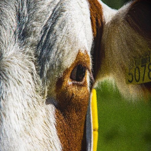
4                                                                                                                  Jiebin Yan 1 et al.

Interestingly, this dataset is still in active use for the de-     well on the training set and i.i.d. test set due to the dataset
velopment of CNN-based edge detection methods (Xie and             insufficiency or selection bias, but fail to generalize to chal-
Tu, 2015). Mikolajczyk and Schmid (2005) conducted a sys-          lenging testing environments. Geirhos et al. (2018) showed
tematic performance evaluation of several local descriptors        that CNNs trained on ImageNet are overly relying on texture
on a set of images with different geometric and photometric        appearances, instead of object shapes as used by humans for
transformations, e.g., viewpoint change and JPEG compres-          image classification. To leverage the spotted shortcut, Bren-
sion. The scale-invariant feature transform (SIFT) (Lowe,          del and Bethge (2019) proposed a learnable bag-of-feature
2004) cut a splendid figure in this synthetic dataset with eas-    model to classify an image by “counting texture patches”
ily inferred ground-truth correspondences. This turned out         without considering their spatial ordering, and achieved high
to be a huge success in computer vision. Similar dataset-          performance on ImageNet.
driven breakthroughs include the structural similarity index            Recently, researchers began to create various fixed out-
(Wang et al., 2004) for image quality assessment thanks            of-distribution (o.o.d.) test sets to probe model generaliz-
to the LIVE database (Sheikh et al., 2006), deformable             ability mainly in the area of image classification. Here, we
part models (Felzenszwalb et al., 2009) for object detection       use the o.o.d. test set to broadly include: 1) samples that
thanks to the PASCAL VOC (Everingham et al., 2015), and            are drawn from the same underlying distribution of the i.i.d.
CNNs for image classification (and general computer vision         training and test data, but belong to different subpopulations
tasks) thanks to the ImageNet (Deng et al., 2009).                 (Jacobsen et al., 2018), and 2) samples that are from a sys-
     Nowadays, nearly all computer vision methods rely on          tematically different distribution. For example, Hendrycks
human-labeled data for algorithm development. As a result,         et al. (2019) compiled a set of natural adversarial examples
the de facto means of probing generalization is to split the       that represent a hard subpopulation of the space of all nat-
available dataset into two (or three) subsets: one for train-      ural images, causing ImageNet classifiers to degrade signif-
ing, (one for validation), and the other for testing. To fa-       icantly. Hendrycks and Dietterich (2019) evaluated the ro-
cilitate fair comparison, the splitting is typically fixed. The    bustness of ImageNet classifiers to common corruptions and
goodness of fit on the test set provides an approximation to       perturbations, such as noise, blur, and weather. Geirhos et al.
generalization beyond training. Recent years have witnessed        (2018) proposed to use synthetic stimuli of conflicting cues
the successful application of the independent and identi-          by transferring the textures of one object (e.g., an Indian ele-
cally distributed (i.i.d.) evaluation to monitor the progress of   phant) to another object (e.g., a tabby cat), while keeping the
many subfields of computer vision, especially where large-         main structures. Li et al. (2017) tested classifiers on sketch,
scale labeled datasets are available.                              cartoon, and painting domains. Although these fixed o.o.d.
     Despite demonstrated successes, computer vision re-           test sets successfully reveal some shortcuts of image clas-
searchers began to reflect on several pitfalls of their evalua-    sifiers, they suffer from the potential problem of extensive
tion strategy. First, the test sets are pre-selected, fixed, and   re-use, similar as fixed i.i.d. test sets.
re-used. This leaves open the door for adapting methods to              Over decades, Ulf Grenander suggested to study com-
the test sets (intentionally or unintentionally) via extensive     puter vision from the pattern theory perspective (Grenander,
hyperparameter tuning, raising the risk of overfitting. For ex-    2012a,b,c). Mumford (1994) defined pattern theory as:
ample, the ImageNet Large Scale Visual Recognition Chal-               The analysis of the patterns generated by the world in
lenge (Russakovsky et al., 2015) was terminated in 2017,               any modality, with all their naturally occurring complex-
which might give us an impression that image classifica-               ity and ambiguity, with the goal of reconstructing the
tion has been solved. Yet Recht et al. (2019) investigated the         processes, objects and events that produced them.
generalizability of ImageNet-trained classifiers by building       According to the pattern theory, if one wants to test whether
a new test set with the same protocol of ImageNet. They,           a computational method relies on intended (rather than
however, found that the accuracy drops noticeably (from            shortcut) features for a specific vision task, the set of fea-
11% to 14%) for a broad range of image classifiers. This re-       tures should be tested in a generative (not a discriminative)
veals the much underestimated difficulty of ensuring a suf-        way. This is the idea of “analysis by synthesis”, and is well-
ficiently representative and unbiased test set. The situation      demonstrated in the field of texture modeling (Julesz, 1962).
would only worsen if human labeling requires extensive do-         Specifically, classification based on some fixed example tex-
main expertise (e.g., medical applications (Jia et al., 2019)),    tures provides a fairly weak test of the sufficiency of a set of
or if failures are rare but fatal in high-stakes and failure-      statistics in capturing the appearances of visual textures. A
sensitive applications (e.g., autonomous cars (Chen et al.,        more efficient test is trying to synthesize a texture image by
2020b; Mohseni et al., 2019)).                                     forcing it to satisfy the set of statistical constraints given by
     More importantly, the i.i.d. evaluation method may not        an example texture image (Portilla and Simoncelli, 2000). If
reveal the shortcut learning problem (Zhang et al., 2019b),        the synthesized image looks identical to the example image
where shortcuts mean a set of decision rules that perform          for a wide variety of texture patterns, the candidate set of
Exposing Semantic Segmentation Failures via Maximum Discrepancy Competition                                                                       5

Fig. 1 The pipeline of the MAD competition for semantic segmentation. (a) A web-scale image set D that provides a closer approximation to
the space of all possible natural images. It is worth noting that dense labeling each image in D is prohibitively expensive (if not impossible). (b)
The MAD image set S ⊂ D, in which each image is able to best discriminate two out of J semantic segmentation models. S is constructed by
maximizing the discrepancy between two models while satisfying a set of constraints to ensure the diversity of exposed failures. The size of S can
be adjusted to accommodate the available human labeling budget. (c) Representative images from S together with the ground-truth maps and the
predictions associated with the two segmentation models. Although many of the chosen models have achieved excellent performance on PASCAL
VOC, MAD is able to automatically expose their respective failures, which are in turn used to rank their generalization to the open visual world.

features is probably sufficient (i.e., intended) to characterize            versing the roles of the two models. The synthesized images
the statistical regularities of visual textures, and is also ex-            are the most informative in revealing their relative advan-
pected to perform well in the task of texture classification.               tages and disadvantages. Nevertheless, the image synthesis
By contrast, if the set of features is insufficient for texture             process may be computationally expensive, and the synthe-
synthesis, the synthesized image would satisfy the identical                sized images may be highly unnatural and of less practical
statistical constraints, but look different. In other words, a              relevance. Ma et al. (2020) alleviated these issues by re-
strong failure of the texture model under testing is identified,            stricting the sampling process from the space of all possible
which is highly unlikely to be included in the pre-selected                 images to a large-scale image subdomain of interest. Wang
and fixed test set for the purpose of texture classification.               et al. (2020) extended this idea to compare multiple Ima-
                                                                            geNet classifiers, where the discrepancy between two classi-
    The recent discovery of adversarial samples (Goodfel-
                                                                            fiers is measured by a weighted hop distance over the Word-
low et al., 2014) of CNN-based image classifiers can also be
                                                                            Net hierarchy (Miller, 1998). However, the above methods
cast into the framework of “analysis by synthesis”. That is,
                                                                            do not take into full consideration the diversity of the se-
imperceptible perturbations are added to synthesize o.o.d.
                                                                            lected samples, which is crucial for fully characterizing er-
images, leading to well-trained classifiers to make wrong
                                                                            roneous corner-case behaviors of the competing models.
predictions. Jacobsen et al. (2018) described a means of syn-
                                                                                 We conclude this section by mentioning that similar
thesizing images that have exact the same probabilities over
                                                                            ideas have emerged in software engineering, in the form of
all 1, 000 classes (i.e., logits), but contain arbitrary object.
                                                                            differential testing (McKeeman, 1998). It is a classic idea to
Segmentation models also suffer from large performance
                                                                            find bug-exposing test samples, by providing the same tests
drop under adversarial examples. Arnab et al. (2018) in-
                                                                            to multiple software implementations of the same function.
vestigated the sensitivity of segmentation methods to ad-
                                                                            If some implementation runs differently from the others, it is
versarial perturbations, and observed that residual connec-
                                                                            likely to be buggy. Inspired by differential testing, Pei et al.
tion and multi-scale processing contribute to robustness im-
                                                                            (2017) developed DeepXplore, an automated whitebox test-
provement. Guo et al. (2019) found that image degradation
                                                                            ing of deep driving systems on synthetic weather conditions.
has a great impact on segmentation models.
     The closest work to ours is due to Wang and Simoncelli
(2008), who practiced “analysis by synthesis” in the field of               3 Proposed Method
computational vision, and proposed the maximum differen-
tiation competition method for efficiently comparing com-                   In this section, we investigate the generalizability of seman-
putational models of perceptual quantities. In the context of               tic segmentation methods by efficiently exposing their fail-
image quality assessment (Wang and Bovik, 2006), given                      ures using the MAD competition (Ma et al., 2020; Wang
two image quality models, they first synthesized a pair of                  and Simoncelli, 2008). Rather than creating another fixed
images that maximize (and minimize) the predictions of one                  test set with human annotations, we automatically sample a
model while fixing the other. This process is repeated by re-               small set of algorithm-dependent images by maximizing the
6                                                                                                                             Jiebin Yan 1 et al.

                                  (a)                                                                    (b)

                                  (c)                                                                    (d)

Fig. 2 An illustration of three plausible outcomes of the MAD competition between two segmentation methods (DeepLabv3+ (Chen et al.,
2018b) and EMANet (Li et al., 2019)). (a) Both methods give satisfactory segmentation results. (b) and (c) One method makes significantly better
prediction than the other. (d) Both methods make poor predictions.

discrepancy between the methods, as measured by common                    budget. The MAD competition suggests to select x̂ by max-
metrics in semantic segmentation (e.g., mean intersection                 imizing the discrepancy between the predictions of the two
over union (mIoU)). Moreover, we allow the resulting MAD                  methods, or equivalently minimizing their concordance:
set to cover diverse sparse mistakes by enforcing a set of ad-
ditional conditions. Subjective testing indicates the relative
performance of the segmentation methods in the MAD com-                   x̂ = arg min S(f1 (x), f2 (x)),                                    (1)
                                                                                  x∈D
petition, where a better method is more aggressive in spot-
ting others’ failures and more resistant to others’ attacks.
The pipeline of the proposed method is shown in Fig. 1.                   where S(·) denotes a common metric in semantic segmen-
                                                                          tation, e.g., mIoU. Comparison of f1 (x̂) and f2 (x̂) against
                                                                          the human-labeled f (x̂) leads to three plausible outcomes:
3.1 The MAD Competition Procedure
                                                                              Case I: Both methods give satisfactory results (see Fig. 2
We formulate the general problem of exposing failures in se-                  (a)). This could happen in theory, for example if both f1
mantic segmentation as follows. We assume a natural image                     and f2 are nearly optimal, approaching the human-level
set D = {x(m) }M     m=1 of an arbitrarily large size, M , whose              performance. In practice, we would like to minimize this
purpose is to approximate the open visual world. For sim-                     possibility since the selected x̂ is not the counterexam-
plicity, each x ∈ D contains N pixels, x = {xn }N      n=1 . Also             ple of either method. This can be achieved by constantly
assumed is a subjective experimental environment, where                       increasing the size of the unlabeled set D while ensuring
                                                       (m)
we can associate each pixel with a class label f (xn ) ∈ Y                    the design differences of f1 and f2 .
for n ∈ {1, 2 . . . , N }, m ∈ {1, 2, . . . , M }, and Y =
{1, 2, . . . , |Y|}. Moreover, we are given J semantic segmen-                Case II: One method (e.g., f1 ) makes significantly bet-
tation models F = {fj }Jj=1 , each of which accepts x ∈ D                     ter prediction than the other (e.g., f2 ). That is, we have
as input, and makes a dense prediction of f (x) ∈ Y N , col-                  successfully exposed a strong failure of f2 with the help
lectively denoted by {fj (x)}Jj=1 . The ultimate goal is to                   of f1 (see Figs. 2 (b) and (c)). The selected x̂ is the most
expose the failures of F and compare their relative perfor-                   valuable in ranking their relative performance.
mance under a minimum human labeling budget.
                                                                              Case III: Both methods make poor predictions, mean-
3.1.1 Main Idea                                                               ing that we have automatically spotted a strong failure
                                                                              of both f1 and f2 (see Fig. 2 (d)). Although the selected
We begin with the simplest scenario, where we plan to ex-                     x̂ offers useful information on how to improve the com-
pose failures of two semantic segmentation methods f1 and                     peting models, it contributes less to the relative perfor-
f2 . We are allowed to collect the ground-truth map f (x) for                 mance comparison between f1 and f2 .
a single image x ∈ D due to the most stringent labeling
Exposing Semantic Segmentation Failures via Maximum Discrepancy Competition                                                                          7

                                                                         (a)

                                                                         (b)

                                                                        (c)
Fig. 3 An illustration of the set of empirical rules to encourage the diversity of the MAD-selected images in terms of scene content and error
type. In this figure, we compare two top-performing semantic segmentation algorithms on PASCAL VOC (Everingham et al., 2015) - DeepLabv3+
(Chen et al., 2018b) and EMANet (Li et al., 2019). The S(·) in Eq. (1) is implemented by mIoU. (a) The MAD samples without any constraints.
It is not hard to observe that objects of the same categories and large scales appear much more frequently. (b) The MAD samples by adding the
category constraint. The proposed method is refined to dig images of different categories, but still falls short in mining objects of different scales.
(c) The MAD samples by further adding the scale constraint, which are more diverse in objective category and scale, therefore increasing the
possibility of exposing different types of corner-case failures.

3.1.2 Selection of Multiple Images                                             shows such an example, where we compare DeepLabv3+
                                                                               (Chen et al., 2018b) and EMANet (Li et al., 2019). The four
It seems trivial to extend the MAD competition using mul-                      samples in sub-figure (a) are representative among the top-
tiple images by selecting top-K images that optimize Eq.                       30 images selected by MAD. We find that objects of the
(1). However, this naı̈ve implementation may simply expose                     same categories (e.g., dining table and potted plant) and ex-
different instantiations of the same type of errors. Fig. 3 (a)
8                                                                                                                                Jiebin Yan 1 et al.

     Algorithm 1: The MAD Competition for Semantic                         Algorithm 2: Adding a New Segmentation Method
     Segmentation                                                          into the MAD Competition
         Input: A large-scale unlabeled image set D, a list of semantic        Input: The same unlabeled image set D, a new segmentation
                 segmentation models F = {fj }J  j=1 , and a                           model fJ+1 , the aggressiveness and resistance
                 concordance measure S                                                 matrices A, R ∈ RJ×J for F ∈ {fj }J   j=1 , and a
         Output: Two global ranking vectors µ(a) , µ(r) ∈ RJ                           concordance measure S
                                                                                                                (a)  (r)
    1    S ← ∅, A ← I, and R ← I {I is the J × J identity matrix}              Output: Two ranking
                                                                                                    vectors µ , µ     ∈ RJ+1
    2    for i ← 1 to J do                                                                0      A 0           0     R 0
                                                                           1   S ← ∅, A ← T            , and R ← T
     3        Compute the segmentation results {fi (x)|x ∈ D}                                    0 1                0 1
    4    end                                                               2   Compute the segmentation results {fJ+1 (x), x ∈ D}
    5    for i ← 1 to J do                                                 3   for i ← 1 to J do
     6        for j ← 1 to J do                                            4        Compute the concordance {S(fi (x), fJ+1 (x))|x ∈ D}
     7             while j 6= i do                                         5        Select fi and fJ+1 as the defender and the attacker,
     8                 Compute the concordance                                       respectively
                        {S(fi (x), fj (x))|x ∈ D}                                                                         n
                                                                                                                             (y)
                                                                                                                                    o|Y|
                                                                           6        Divide D into |Y| overlapping groups Di,J+1
     9                 Divide D into |Y| overlapping groups                                                                             y=1
                        n
                             (y) |Y|
                                o                                                    based on the predictions of the defender
                          Dij         based on the predictions of fi       7       for y ← 1 to |Y| do
                                    y=1
                           (i.e., fi is the defender)                                           (y)
                                                                           8            Filter Di,J+1 according to the scale constraint
    10                   for y ← 1 to |Y| do                                                                       (y)
                                         (y)                               9           Create the MAD subset Si,J+1 by selecting top-K
    11                         Filter Dij according to the scale                                                  (y)
                                 constraint                                             images in the filtered   Di,J+1   that optimize Eq. (2)
                                                        (y)                                   S (y)
    12                         Create the MAD subset Sij by selecting     10           S ← S Si,J+1
                                                             (y)
                                top-K images in the filtered Dij that     11       end
                                optimize Eq. (2)                          12       Switch the roles of fi and fJ+1 , and repeat Step 6 to
                                      S (y)                                         Step 10
    13                         S ← S Sij
                                                                          13   end
    14                   end
                                                                          14   Collect human segmentation maps for S
    15             end
                                                                          15   for i ← 1 to J do
    16       end                                                          16        a0i,J+1 ← P (fi ; SJ+1,i )/P (fJ+1 ; SJ+1,i )
 17      end                                                              17        a0J+1,i ← P (fJ+1 ; Si,J+1 )/P (fi ; Si,J+1 )
 18      Collect human segmentation maps for S                                       0
 19      Compute the aggressiveness matrix A and the resistance           18        ri,J+1  ← P (fi ; Si,J+1 )/P (fJ+1 ; Si,J+1 )
                                                                                     0
          matrix R using Eq. (3) and Eq. (5), respectively                19        rJ+1,i  ← P (fJ+1 ; SJ+1,i )/P (fi ; SJ+1,i )
 20      Aggregate paired comparison results into two global ranking      20   end
          vectors µ(a) and µ(r) by maximum likelihood estimation          21   Update the two global ranking vectors µ(a) and µ(r)

tremely large scales (e.g., occupying the entire image) fre-
quently occur, which makes the comparison less interesting
and useful. Here we enforce a category constraint to encour-          the MAD samples associated with DeepLabv3+ (Chen et al.,
age more diverse images to be selected in terms of scene              2018b) and EMANet (Li et al., 2019), when we add the cate-
content and error type. Specifically, we set up a defender-           gory constraint. As expected, objects of different categories
attacker game, where the two segmentation models, f1 and              begin to emerge, but the selection is still biased towards ob-
f2 , play the role of the defender and the attacker, respec-          jects with relatively large scales. To mitigate this issue, we
tively. We divide the unlabeled set D into |Y| overlapping            add a second scale constraint. Suppose that all competing
            (y) |Y|
groups {D12 }y=1 according to the predictions by the de-              models use the same training set L, which is divided into
                                                                                          |Y|
fender f1 : if f1 (xn ) = y, for at least one spatial location        |Y| groups {L(y) }y=1 based on the ground-truth segmenta-
                                  (y)
n ∈ {1, 2, . . . , N }, then x ∈ D12 . After that, we divide the      tion maps. For x ∈ L(y) , we count the proportion of pixels
optimization problem in (1) into |Y| subproblems:                     that belong to the y-th object category, and extract the first
                                                                                 (y)                          (y)
  (k)                                                                 quartile Tmin and the third quartile Tmax as the scale statis-
x̂ =          arg min       S(f1 (x), f2 (x)), ∀y ∈ {1, . . . , |Y|},                   (y) S (y)
             (y)
         x∈D12 \{x̂(m) }k−1
                        m=1
                                                                      tics. For x ∈ D12       D21 , if the proportion of pixels be-
                                                                                                                      (y)   (y)
                                                                (2)   longing to the y-th category is in the range [Tmin , Tmax ], x is
                                                                      valid for comparison of f1 and f2 . Otherwise, x will be dis-
where {x̂(m) }k−1m=1 is the set of k − 1 images that have al-         carded. Fig. 3 (c) shows the MAD samples of DeepLabv3+
ready been identified. We may reverse the role of f1 and              and EMANet by further adding the scale constraint. As can
                        (y) |Y|
f2 , divide D into {D21 }y=1 based on f2 which is now the             be seen, objects of different categories and scales have been
defender, and solve a similar set of optimization problems            spotted, which may correspond to failures of different un-
                                           (y)
to find top-K images in each subset D21 . Fig. 3 (b) shows            derlying root causes.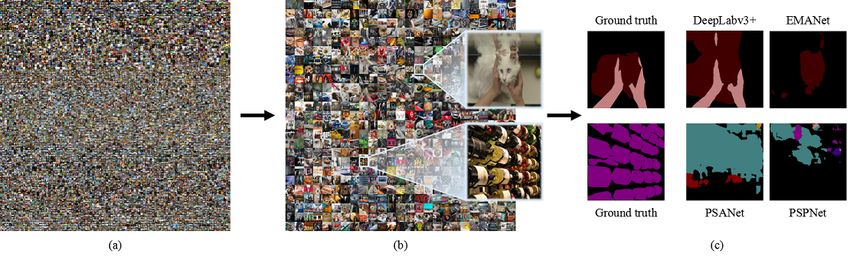
Exposing Semantic Segmentation Failures via Maximum Discrepancy Competition 9
3.1.3 Comparison of Multiple Models Table 1 The object categories in the PASCAL VOC benchmark (Ev-
eringham et al., 2015).
We further extend the MAD competition to include J seg- Category
mentation models. For each out of J × (J − 1) ordered Person person
pairs of segmentation models, fi and fj , where i 6= j and Animal bird, cat, cow, dog, horse, sheep
i, j ∈ {1, 2 . . . , J}, we follow the procedure described in Vehicle aero plane, bicycle, boat, bus, car, motorbike, train
(y) |Y| bottle, chair, dining table, potted plant, sofa,
Section 3.1.2 to obtain |Y| MAD subsets {Sij }y=1 , where Indoor
tv/monitor
(y) (y)
Sij contains top-K images from Dij with fi and fj being
the defender and the attacker, respectively. The final MAD
S (y) Table 2 The first and third quartiles of the scale statistics for each
set S = Sij has a total of J × (J − 1) × |Y| × K images, category in PASCAL VOC (Everingham et al., 2015).
whose number is independent of the size of the large-scale
unlabeled image set D. This nice property of MAD encour- Category Tmin Tmax Category Tmin Tmax
aero plane 0.034 0.160 bicycle 0.013 0.087
ages us to expand D to include as many natural images as bird 0.021 0.148 boat 0.031 0.158
possible, provided that the computational cost for dense pre- bottle 0.006 0.148 bus 0.167 0.450
diction is negligible. car 0.018 0.262 cat 0.129 0.381
After collecting the ground-truth segmentation maps for chair 0.021 0.129 cow 0.069 0.292
potted plant 0.079 0.286 sheep 0.076 0.302
S (details in Section 4.1.4), we compare the segmentation
sofa 0.082 0.284 train 0.082 0.264
models in pairs by introducing the notions of aggressive- tv/monitor 0.027 0.249 dining table 0.012 0.109
ness and resistance (Ma et al., 2020). The aggressiveness dog 0.039 0.297 horse 0.084 0.262
aij quantifies how aggressive fi is to identify the failures of motorbike 0.132 0.356 person 0.028 0.199
fj as the attacker:
P (fi ; Sji ) where Φ(·) is the standard Gaussian cumulative distribu-
aij = , (3)
P (fj ; Sji ) tion function. Direct optimization of L(µ(a) |A) suffers from
the translation ambiguity. To obtain a unique solution, one
where P (a)
often adds an additional constraint that i µi = 1 (or
(a)
|Y| µ1 = 0). The vector of global resistance scores µ(r) ∈ RJ
1 X 1 X
P (fi ; Sji ) = S(fi (x), f (x)) . can be obtained in a similar way. We summarize the MAD
|Y| y=1 S (y)
ji (y)
x∈Sji competition procedure in Algorithm 1.
(4) Last, we note that a new semantic segmentation algo-
rithm fJ+1 can be easily added into the current MAD com-
Note that a small positive constant may be added to both petition. The only additional work is to 1) select MAD
the numerator and the denominator of Eq. (3) as a form of subsets by maximizing the discrepancy between fJ+1 and
Laplace smoothing to avoid potential division by zero. aij F, subject to the category and scale constraints, 2) collect
is nonnegative with a higher value indicating stronger ag- ground-truth dense labels for the newly selected images, 3)
gressiveness. The resistance rij measures how resistant fi is expand A and R by one to accommodate new paired com-
against the attack from fj : parison results, and 4) update the two global ranking vectors
(see Algorithm 2).
P (fi ; Sij )
rij = (5)
P (fj ; Sij )
with a higher value indicating stronger resistance. The pair- 4 Experiments
wise aggressiveness and resistance statistics of all J seg-
mentation models form two J × J matrices A and R, re- In this section, we apply the MAD competition to com-
spectively, with ones on diagonals. Next, we convert pair- pare ten semantic segmentation methods trained on PAS-
wise comparison results into global rankings using maxi- CAL VOC (Everingham et al., 2015). We focus primarily
mum likelihood estimation (Tsukida and Gupta, 2011). Let- on PASCAL VOC because 1) it is a well-established bench-
(a) (a) (a)
ting µ(a) = [µ1 , µ2 , . . . , µJ ] be the vector of global ag- mark accompanied by many state-of-the-art methods with
gressive scores, we define the log-likelihood of the aggres- different design modules, therefore providing a comprehen-
sive matrix A as sive pictures of the segmentation methods’ pros and cons;
and 2) the performance on this benchmark seems to have
(a) (a)
X
L(µ(a) |A) = aij log Φ µi − µj , (6) saturated, therefore questioning demanding finer discrimi-
ij nation between segmentation methods.
10                                                                                                                   Jiebin Yan 1 et al.

 RefineNet/EMANet    BlitzNet/RefineNet

PSANet/DeepLabv3+     PSPNet/PSANet

RefineNet/ESPNetv2 PSPNet/LRefineNet

Fig. 4 “Boat” images selected from D by MAD (left panel) and from PASCAL VOC (right panel). Shown below each MAD image are the two
associated segmentation methods.

LRefineNet/EMANet    PSPNet/RefineNet

     FCN/ESPNetv2    PSPNet/EMANet

 PSANet/LRefineNet   PSPNet/ESPNetv2

Fig. 5 “Person” images selected from D by MAD (left panel) and from PASCAL VOC (right panel).

4.1 Experimental Setup                                               4.1.2 Construction of F

4.1.1 Construction of D                                              In this study, we test ten CNN-based semantic segmenta-
                                                                     tion models trained on PASCAL VOC (Everingham et al.,
                                                                     2015), including FCN (Long et al., 2015), PSPNet (Zhao
                                                                     et al., 2017), RefineNet (Lin et al., 2017), BlitzNet (Dvornik
Before introducing the unlabeled image set D, we first               et al., 2017), DeepLabv3+ (Chen et al., 2018b), LRe-
briefly review the PASCAL VOC benchmark (Everingham                  fineNet (Nekrasov et al., 2018), PSANet (Zhao et al.,
et al., 2015). It contains 20 object categories as listed in Ta-     2018b), EMANet (Li et al., 2019), DiCENet (Mehta et al.,
ble 1. The first and third quartiles of the scale statistics for     2019a) and ESPNetv2 (Mehta et al., 2019b), which are cre-
each category are given in Table 2. The number of training           ated from 2015 to 2019. Among the test methods, FCN
and validation images are 1, 464 and 1, 149, respectively. We        is a pioneering work in deep semantic segmentation. LRe-
follow the construction of PASCAL VOC, and crawl web                 fineNet is a faster version of RefineNet. Therefore, it is inter-
images using the same category keywords, their synonyms,             esting to see the trade off between speed and accuracy under
as well as keyword combinations (e.g., person + bicycle). No         the MAD setting. It is also worth investigating the effects
data screening is needed during data crawling. In our exper-         of several core modules, such as dilated convolution, skip
iment, we build D with more than 100, 000 images, which              connection, multi-scale computation, and attention mecha-
is substantially larger than the training and validation sets of     nism to enhance model robustness when facing the open vi-
PASCAL VOC. Some MAD images from D are shown in                      sual world. For all segmentation models, we use the publicly
Figs. 4 and 5, in contrast to images of the same categories in       available implementations with pre-trained weights to guar-
PASCAL VOC.                                                          antee the reproducibility of the results on PASCAL VOC
Exposing Semantic Segmentation Failures via Maximum Discrepancy Competition 11
Fig. 6 The pie chart of the mIoU values of all ten segmentation meth-
ods on the MAD set S.
Fig. 7 The box-plot of the mIoU values of individual segmentation
methods. We evaluate fi on two disjoint and complementary subsets
(see Table 3). In all experiments, we resize the input image Ui and Vi of S, where Ui and Vi include images that are associated
to 512 × 512 for inference. with and irrelevant to fi , respectively. The gray bar represents the me-
dian mIoU. The lower and upper boundaries of the box indicate the first
and third quartiles, respectively. The minimum and maximum data are
4.1.3 Construction of S
also shown as the endpoints of the dashed line.
To construct S, we need to specify the concordance metric
in Eq. (1). In the main experiments, we adopt mIoU, which 4.1.4 Subjective Annotation
is defined as
|Y| We invite seven participants to densely label the MAD im-
1 X Nyy
mIoU = P|Y| P|Y| , ages with the help of the graphical image annotation tool -
|Y| + 1 y=0
y 0 =0 Nyy 0 + y 0 =0 Ny 0 y − Nyy LabelMe2 . To familiarize participants with the labeling task,
(7) we include a training session to introduce general knowl-
where the mean is taken over all object categories, and edge about semantic segmentation and the manual of La-
belMe. As suggested in PASCAL VOC, we perform two
N
X rounds of subjective experiments. The first round of experi-
Nyy0 = I[fi (xn ) = y ∩ fj (xn ) = y 0 ], (8)
ment is broken into multiple sessions. In each session, par-
n=1
ticipants are required to annotate 20 images, followed by a
where I[·] denotes the indicator function. In Section 4.3, we short break to reduce the fatigue effect. Participants can dis-
will investigate the sensitivity of the results when we switch cuss with each other freely, which contributes to the annota-
to other metrics commonly used in semantic segmentation, tion consistency. In the second round, we carry out cross val-
such as mean accuracy. idation to further improve the consistency of the annotated
As no data cleaning is involved in the construction of D, data. Each participant takes turn to check the segmentation
it is possible that the selected MAD images fall out of the maps completed by others, marking positions and types of
20 object categories (e.g., elephants), or are unnatural (e.g., possible annotation errors. During this process, participants
cartoons). In this paper, we restrict our study to test the gen- can also communicate with each other. After sufficient dis-
eralizability of semantic segmentation models to subpopu- cussions among participants, disagreement on a small por-
lation shift (Santurkar et al., 2020), and only include natu- tion of annotations is thought to be aligned.
ral photographic images containing the same 20 object cat-
egories. This is done in strict adherence to the data prepara-
tion guideline of PASCAL VOC (Everingham et al., 2015).
4.2 Main Results
As will be clear in Section 4.2, this seemingly benign setting
already poses a grand challenge to the competing models. We first get an overall impression on the model generaliz-
Considering the expensiveness of subjective testing, we set ability by putting together the mIoU values obtained by all
K = 1, which corresponds to selecting the optimal image ten segmentation methods on the MAD set S in Fig. 6. It is
to discriminate between each ordered pair of segmentation clear that MAD successfully exposes failures of these CNN-
models in each object category. After removing repetitions,
S includes a total of 833 images. 2
https://github.com/wkentaro/labelme12 Jiebin Yan 1 et al.
Fig. 8 An illustration of MAD failure transferability. The natural photographic image in the left panel is selected by MAD to best differentiate
BlitzNet (Dvornik et al., 2017) and ESPNetv2 (Mehta et al., 2019b). Interestingly, it is also able to falsify other competing models in dramatically
different ways, as shown in the right panel.
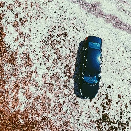
Fig. 9 The aggressiveness matrix A computed by Eq. (3) to indicate Fig. 10 The resistance matrix R computed by Eq. (5) to indicate how
how aggressive the row model is to falsify the column model. A larger resistant the row model is under attack by the column model. A larger
value with cooler color indicates stronger aggressiveness. value with cooler color indicates stronger resistance.
based methods, leading to a substantial performance drop two associated segmentation methods (i.e., falling in Case
on S. More precisely, over 84.7% of the mIoU values are III). Second, the performance of fi on Vi is only slightly
smaller than 0.6, while less than 8% exceed 0.8 (see Fig. 6). better than that on Ui , suggesting that the MAD images are
This is in stark contrast to the pronounced results on PAS- highly transferable to falsify other segmentation models (see
CAL VOC, where all ten methods achieve an mIoU value Fig. 8). This coincides with the strong transferability of ad-
greater than 0.6 (see Table 3). We next take a closer look at versarial examples (often with imperceptible perturbations)
individual performance. For each segmentation method fi , found in image classification. In summary, MAD has iden-
we divide S into two disjoint subsets Ui and Vi , where im- tified automatically a set of naturally occurring hard exam-
ages in Ui and Vi are associated with and irrelevant to fi , ples from the open visual world that significantly degrade
respectively. We evaluate fi on the two subsets, and summa- segmentation accuracy.
rize the mIoU results in Fig. 7, from which we have two in- We continue to analyze the aggressiveness and resis-
sightful observations. First, the performance of fi on Ui for tance of the test methods when they compete with each
all i = {1, 2, . . . , J} is marginal, indicating that a significant other in MAD. We first show the aggressiveness and resis-
portion of the MAD images are double-failure cases of the tance matrices, A and R, in Figs. 9 and 10, respectively.Exposing Semantic Segmentation Failures via Maximum Discrepancy Competition 13
Table 3 The performance comparison of ten semantic segmentation models. A and R represent aggressiveness and resistance, respectively.
Model Backbone mIoU mIoU rank A rank ∆A rank R rank ∆R rank
DeepLabv3+ (Chen et al., 2018b) Xception 0.890 1 1 0 1 0
EMANet (Li et al., 2019) ResNet-152 0.882 2 5 -3 5 -3
PSANet (Zhao et al., 2018b) ResNet-101 0.857 3 6 -3 6 -3
PSPNet (Zhao et al., 2017) ResNet-101 0.854 4 8 -4 9 -5
LRefineNet (Nekrasov et al., 2018) ResNet-152 0.827 5 4 +1 4 +1
RefineNet (Lin et al., 2017) ResNet-101 0.824 6 2 +4 3 +3
BlitzNet (Dvornik et al., 2017) ResNet-50 0.757 7 3 +4 2 +5
ESPNetv2 (Mehta et al., 2019b) - 0.680 8 7 +1 7 +1
DiCENet (Mehta et al., 2019a) - 0.673 9 9 0 8 +1
FCN (Long et al., 2015) VGG16 0.622 10 10 0 10 0
A higher value in each entry with cooler color represents Third, the rankings of both EMANet (Li et al., 2019) and
stronger aggressiveness/resistance of the corresponding row PSANet (Zhao et al., 2018b) drop slightly in MAD com-
model against the column model. From the figures, we make pared with their excellent performance on PASCAL VOC.
two interesting observations. First, it is relatively easier for This reinforces the concern that “delicate and advanced”
a segmentation method to attack other methods than to sur- modules proposed in semantic segmentation (e.g., the atten-
vive the attack from others, as indicated by the larger values tion mechanisms used in EMANet and PSANet) may have
in A than those in R. Second, a segmentation method with a high risk of overfitting to the extensively re-used bench-
stronger aggressiveness generally shows stronger resistance, marks. As a result, the generalizability of EMANet and
which is consistent with the finding in the context of im- PSANet to the open visual world is inferior to segmentation
age quality assessment (Ma et al., 2020). We next aggregate models with simpler design, such as BlitzNet.
paired comparisons into global rankings, and show the re- Fourth, the MAD performance of some low-weight ar-
sults in Table 3. We have a number of interesting findings, chitectures, ESPNetv2 and DiCENet, are worse than the
which are not apparently drawn from the high mIoU num- competing models except FCN, which is consistent with
bers on PASCAL VOC. their performance on PASCAL VOC. These results indi-
cate that the trade-off between computational complexity
First, although BlitzNet (Dvornik et al., 2017) focuses
and segmentation performance should be made in practice.
on improving the computational efficiency of semantic seg-
We conclude by visualizing the MAD failures of the seg-
mentation with below-the-average mIoU performance on
mentation models in Fig. 11, where mIoU < 0.6. Generally,
PASCAL VOC, it performs remarkably well in compari-
the selected images are visually much harder, containing
son to other models in MAD. A distinct characteristic of
novel appearances, untypical viewpoints, extremely large or
BlitzNet is that it employs object detection as an auxiliary
small object scales, and only object parts.
task for joint multi-task learning. It is widely acceptable
that object detection and semantic segmentation are closely
related. Early researchers (Leibe et al., 2004) used detec- 4.3 Ablation Studies
tion to provide a good initialization for segmentation. In
the context of end-to-end optimization, we conjecture that 4.3.1 Sensitivity of Different Performance Measures
the detection task would regularize the segmentation task to
learn better localized features for more accurate segmenta- We conduct ablation experiments to test the sensitivity of
tion boundaries. Another benefit of this multi-task setting MAD results to different performance measures in Eq. (2).
is that BlitzNet can learn from a larger number of images Apart from mIoU, we adopt another two commonly used
through the detection task, with labels much cheaper to ob- criteria in semantic segmentation, the frequency weighted
tain than the segmentation task. IoU (FWIoU) and the mean pixel accuracy (MPA), which
are defined as
Second, RefineNet (Lin et al., 2017) shows strong com-
P|Y| Nyy
petence in MAD, moving up at least three places in the ag- y=0 P|Y| P|Y|
y 0 =0
Nyy0 + y0 =0 Ny0 y −Nyy
gressiveness and resistance rankings. The key to the model’s FWIoU = P|Y| P|Y| , (9)
success is the use of multi-resolution fusion and chained y=0 y 0 =0 Nyy0
residual pooling for high-resolution and high-accuracy pre-
and
diction. This is especially beneficial for segmenting images
that only contain object parts (see Figs. 4, 5 and 11 (d)). |Y|
1 X Nyy
In addition, the chained residual pooling module may also MPA = , (10)
|Y| + 1 y=0 |Y|
P
contribute to making better use of background context. 0 Nyy0
y =014 Jiebin Yan 1 et al.
(a) Appearance.
(b) Viewpoint.
(c) Object scale.
(d) Object part.
Fig. 11 Visualization and summary of common MAD failures of the competing segmentation models.
respectively, where Nyy0 has been specified in Eq. (8). We Table 4 The sensitivity of the MAD rankings to the choice of segmen-
follow the same procedure as in Sections 4.1.3 to construct tation performance measures in Eq. (2). The SRCC values are com-
puted using the aggressiveness and resistance rankings under mIoU as
two MAD sets under FWIoU and MPA, containing 662 and
reference.
825 distinct images, respectively. The subjective annotation
procedure is also in accordance to Section 4.1.4. After col- SRCC
Aggressiveness ranking under FWIoU 0.891
lecting the ground-truth segmentation maps, we compare the
Aggressiveness ranking under MPA 0.878
global aggressiveness and resistance rankings under FWIoU Resistance ranking under FWIoU 0.879
and MPA, with those under mIoU, which serve as reference. Resistance ranking under MPA 0.830
Table 4 shows the Spearman’s rank correlation coefficient
(SRCC) results, which are consistently high, indicating that
the MAD rankings are quite robust to the choice of segmen- 2019a), DANet (Fu et al., 2019a), and Panoptic-DeepLab
tation performance measures. (Cheng et al., 2020), all trained mainly on the Cityscapes
dataset (Cordts et al., 2016). Specifically, HANet includes
an add-on module, with emphasis on the distinct character-
4.4 Further Testing on WildDash
istics of urban-scene images. We test HANet with the back-
bone ResNeXt-101 (Xie et al., 2017) for its optimal per-
We further validate the feasibility of MAD to expose seman-
formance. DGCNet exploits graph convolutional networks
tic segmentation failures on another challenging dataset -
for capturing long-range contextual information. DANet
WildDash (Zendel et al., 2018) with unban-scene images.
uses position attention and channel attention modules, while
This dataset is designed specifically for testing segmenta-
Panoptic-DeepLab adopts the dual-decoder module for se-
tion models for autonomous driving. We download 4, 256
mantic segmentation. We follow the experimental protocols
images from its official website3 to construct D.
on PASCAL VOC with one key difference: we opt to a two-
We test four recent semantic segmentation models, in-
alternative forced choice (2AFC) method to minimize the
cluding HANet (Choi et al., 2020), DGCNet (Zhang et al.,
human labeling effort. In particular, instead of obtaining the
3
https://www.wilddash.cc/ ground-truth segmentation maps for the selected MAD im-Exposing Semantic Segmentation Failures via Maximum Discrepancy Competition 15
Table 5 The MAD competition of four semantic segmentation models rich and diverse failures. We are currently testing this idea,
on WildDash (Zendel et al., 2018). The mIoU results are computed on and preliminary results indicate that existing models are able
Cityscapes (Cordts et al., 2016). A and R represent aggressiveness and
to learn from their MAD failures for improved segmentation
resistance, respectively.
performance. Moreover, if we relax the constraint of densely
Model mIoU/rank A/∆ rank R/∆ rank labeling S and opt for other forms of cheaper labels (e.g.,
HANet 0.832 / 1 1/0 1/0 object bounding boxes), we can significantly enlarge the size
DGCNet 0.820 / 2 4 / -2 4 / -2
DANet 0.815 / 3 2 / +1 2 / +1
of S, which may also be useful for boosting the segmenta-
Panoptic-DeepLab 0.809 / 4 3 / +1 3 / +1 tion performance. In addition, it is also interesting to see
whether the MAD-selected images in the context of seman-
tic segmentation are equally transferable to falsify computa-
ages, participants are forced to choose the better prediction tional models of related tasks, such as instance segmentation
from two competing models. Two experienced postgraduate and object detection.
students are invited to this subjective experiment.
We show the global ranking results in Table 5, and make Acknowledgements This work was partially supported by the Na-
two consistent observations, which have been drawn from tional Key R&D Program of China under Grant 2018AAA0100601,
the experiments on PASCAL VOC. First, more training data and the National Natural Science Foundation of China under Grants
leads to improved generalizability. For example, the best- 62071407 and 61822109.
performing HANet is trained on both coarsely and finely an-
notated images in Cityscapes (Cordts et al., 2016) as well as Conflict of interest
Mapillary (Neuhold et al., 2017), while other test models are
only trained on the finely annotated images in Cityscapes. The authors declare that they have no conflict of interest.
Second, the incorporation of “advanced” modules in DGC-
Net, such as graph convolutional networks, may encourage
overfitting to i.i.d. data from Cityscapes, with weak gener- References
alization to o.o.d. data from WildDash. We also show rep-
Arbelaez P, Maire M, Fowlkes C, Malik J (2011) Con-
resentative MAD samples and the four model predictions in
tour detection and hierarchical image segmentation. IEEE
Fig. 12. We find that MAD successfully exposes strong fail-
Transactions on Pattern Analysis and Machine Intelli-
ures of the two associated models, which transfer well to
gence 33(5):898–916
falsify other segmentation methods.
Arnab A, Miksik O, Torr Philio H (2018) On the robustness
of semantic segmentation models to adversarial attacks.
5 Conclusion In: IEEE International Conference on Computer Vision
and Pattern Recognition, pp 888–897
In this paper, we have investigated the generalizability of se- Badrinarayanan V, Kendall A, Cipolla R (2017) SegNet: A
mantic segmentation models by exposing their failures via deep convolutional encoder-decoder architecture for im-
the MAD competition. The main result is somewhat sur- age segmentation. IEEE Transactions on Pattern Analysis
prising: high accuracy numbers achieved by existing seg- and Machine Intelligence 39(12):2481–2495
mentation models on closed test sets do not result in robust Brendel W, Bethge M (2019) Approximating CNNs with
generalization to the open visual world. In fact, most im- bag-of-local-features models works surprisingly well on
ages selected by MAD are double-failures of the two as- ImageNet. arXiv preprint arXiv:190400760
sociated segmentation models with strong transferability to Burt PJ (1981) Fast filter transform for image processing.
falsify other methods. Fortunately, as the MAD samples are Computer Graphics and Image Processing 16(1):20–51
selected to best differentiate between two models, we are Canny J (1986) A computational approach to edge detec-
able to rank their relative performance in terms of aggres- tion. IEEE Transactions on Pattern Analysis and Machine
siveness and resistance through this failure-exposing pro- Intelligence 8(6):679–698
cess. We have performed additional experiments to verify Cao L, Fei-Fei L (2007) Spatially coherent latent topic
that the MAD results are insensitive under different segmen- model for concurrent segmentation and classification of
tation measures, and are consistent across different segmen- objects and scenes. In: IEEE International Conference on
tation datasets. We hope that the proposed MAD for seman- Computer Vision, pp 1–8
tic segmentation would become a standard complement to Chen LC, Papandreou G, Kokkinos I, Murphy K, Yuille
the close-set evaluation of a much wider range of dense pre- AL (2017) DeepLab: Semantic image segmentation with
diction problems. deep convolutional nets, atrous convolution, and fully
A promising future direction is to jointly fine-tune the connected CRFs. IEEE Transactions on Pattern Analysis
segmentation methods on the MAD set S, which contains and Machine Intelligence 40(4):834–848You can also read