Are State Governments Roadblocks to Federal Stimulus? Evidence from Highway Grants in the 2009 Recovery Act
←
→
Page content transcription
If your browser does not render page correctly, please read the page content below
FEDERAL RESERVE BANK OF SAN FRANCISCO

                          WORKING PAPER SERIES

        Are State Governments Roadblocks to Federal
                         Stimulus?
            Evidence from Highway Grants in the
                     2009 Recovery Act

                                 Sylvain Leduc
                     Federal Reserve Bank of San Francisco

                                 Daniel Wilson
                     Federal Reserve Bank of San Francisco

                                  January 2014

                         Working Paper 2013-16
  http://www.frbsf.org/publications/economics/papers/2013/wp2013-16.pdf

The views in this paper are solely the responsibility of the authors and should not be
interpreted as reflecting the views of the Federal Reserve Bank of San Francisco or the
Board of Governors of the Federal Reserve System.
Are State Governments Roadblocks to Federal Stimulus?
Evidence from Highway Grants in the 2009 Recovery Act
Sylvain Leduc and Daniel Wilson (FRB San Francisco)*
January 6, 2014
Abstract
We examine how state governments adjusted spending in response to the large temporary
increase in federal highway grants under the 2009 American Recovery and Reinvestment Act
(ARRA). The mechanism used to apportion ARRA highway grants to states allows us to isolate
exogenous changes in these grants. We find that states increased highway spending in 2010
nearly dollar-for-dollar with their apportioned grants, implying little if any crowd-out. We show
that our results are not unique to the ARRA period, but rather are consistent with a strong effect
from grants dating back at least to the early 1980s.
JEL Codes: H77, H54, E62
*We thank Brian Lucking, Ben Pyle, and Akshay Rao for excellent research assistance. We also thank
Brian Knight for providing the data he used in Knight (2002). The paper benefited from comments from
William Gale, Diane Lim, Teresa Mila-Garcia, David Phillips, and conference and seminar participants at
the Federal Reserve Bank of San Francisco, Urban Economics Association, National Tax Association,
and IEB Workshop on Fiscal Federalism. The views expressed in this paper are solely the responsibility
of the authors and should not be interpreted as reflecting the views of the Federal Reserve Bank of San
Francisco, or of any other person associated with the Federal Reserve System.I. Introduction
Often overlooked in debates about the merits of federal stimulus spending or federal
spending in general is the role of subnational governments as “middlemen,” propagating shocks in
federal spending to the real economy. After all, a significant and growing portion of federal
spending in many countries comes in the form of federal transfers to regional governments that
actually administer the spending. This is particularly true for stimulus spending. For instance,
nearly half of the estimated $550 billion in federal spending from the 2009 American Recovery
and Reinvestment Act (ARRA or Recovery Act) consisted of grants to state governments.
The composition and effects of fiscal expansions, both in general and as countercyclical
tools, depend in large part on what states do with federal grants.1 On the one hand, grants targeted
for a specific purpose such as for highways or education are presumably intended to induce states
to increase spending for that purpose.2 Yet federal grants generally are partially or fully fungible,
allowing states to simply use the grant revenue to substitute for the state’s tax revenue and other
own funds that would have funded that spending, thus enabling states to reduce tax rates or
decrease their net borrowing. This substitution often is referred to as “crowd-out.” While this
paper is agnostic on which of these possible uses of federal grants – spending, tax cuts, or saving –
has the highest economic multiplier, the choice made by state governments is of critical
importance, both to policymakers aiming to achieve the type of fiscal stimulus they intend and to
economists seeking to understand the likely effects of fiscal expansions.
Because the Recovery Act eased the requirements that states must meet to obtain federal
grants, many have argued that crowd-out might have been particularly high in this case and could
have greatly reduced the effect of the legislation on overall government spending. In particular,
mechanisms such as matching requirements that require states to pay a fraction of the costs of a
project otherwise financed with federal grants can reduce crowd-out. But these requirements were
waived for many types of grants under the ARRA. For instance, federal highway grants typically
involve a 20 percent matching requirement, which was waived under the ARRA.
Similarly, requirements that states maintain their own level of funding in order to receive
1
The issue is analogous to how households’ marginal propensity to consume determines the effects of federal
transfers and income tax cuts to individuals. See, for instance, Johnson, Parker, and Souleles (2006) for an analysis
of the income tax rebate of 2001.
2
This oft-documented phenomenon of federal grant revenues stimulating higher expenditures by recipient
subnational governments is known as the “flypaper effect” in the public finance literature. See Inman (2008) for a
recent survey of the literature on the flypaper effect and Hines and Thaler (1995) for an earlier review.
1federal funds (known as maintenance-of-effort requirements) are intended to mitigate crowd-out
effects of federal grants. But these requirements can be difficult to enforce in normal times and
likely are much more difficult to enforce in recessions. Over the 2008-2010 period, in particular,
many state governments underestimated the pace at which their budgetary balances were
deteriorating, leading to strong pressures to reduce expenditures more than previously planned.
The potential crowd-out of states’ own funding by ARRA grants figures importantly in a
number of recent studies of the ARRA. Cogan and Taylor (2011) and Inman (2010) argue, based
on national time series data, that the Recovery Act’s grants failed to provide much economic
stimulus partly because states appear to have responded to higher federal grants for infrastructure,
education, and the like by reducing borrowing, leaving state governments’ spending on goods and
services nearly unchanged.3 Conley and Dupor (forthcoming), in their cross-state analysis of the
employment effects of ARRA spending, make a similar argument, emphasizing that crowd-out
was likely high under ARRA, particularly in the case of highway spending. The Congressional
Budget Office (CBO) also relied on an assumption of partial crowd-out of state spending in its
analysis of the expected fiscal cost of the Recovery Act.4
The concerns are especially relevant for federal highway grants, which Knight (2002)
showed led to nearly complete crowd-out over the period 1983 to 1997. Moreover, highway
spending was roughly flat nationally over the 2008-2011 period, despite the nearly 50 percent
increase in announced grant funding in 2009 resulting from the Recovery Act. While it is difficult
to infer the effect of higher federal grants on state spending by looking at national time series data
alone due to the inability to observe what state spending would have been absent the additional
grants, to many the flatness of national spending over this period is prima facie evidence of high
crowd out.
In this paper, we address the question of crowd-out of federal grants to states by focusing on
ARRA highway grants. We focus on highway grants both because of the a priori reasons
mentioned above to suspect crowd-out and because highway grants afford particularly strong
identification of their causal effects due to the institutional mechanism determining their cross-
3
Likewise, Gramlich (1978), based on national time series patterns in state and local government spending and
saving, concluded that state and local governments saved nearly all of federal transfers they received as part of the
economic stimulus of 1976.
4
See CBO (2009).
2state allocation. We use cross-state data to examine how state governments adjusted their highway
spending in response to the large temporary increase in federal grants under ARRA.
We follow an instrumental variables (IV) difference-in-differences methodology. The first
of the two differences is across time, comparing a given state’s highway spending in 2008, the
year before the ARRA, to its spending in the years after. By time differencing, we remove any
state fixed effects, such as those due to time-invariant state characteristics like density, climate,
and political preferences, which could otherwise influence state-government highway spending.
The second difference involves comparison across states that received different amounts of
highway grants per capita.
We focus primarily on the effect of ARRA highway grants on states highway spending in
2010 both because the ARRA highway grants were not announced until March 2009 and because
previous research has found substantial time lags between highway grant announcements and
outlays (see Leduc and Wilson (2013)). The ARRA stipulated that states must commit ARRA
grant funds to specific projects by September 2010, suggesting that much of the resulting outlays
would occur in 2010. Nonetheless, we also estimate the effects of the ARRA grants on state
highway spending in 2009 and 2011, as well as the cumulative effect over 2009-2011.
Most of the ARRA highway funds were apportioned to states based on long-standing, pre-
existing formulas. These formulas are based on road factors, such as the number of lane miles in a
state or a state’s contribution to the Highway Trust Fund, which are known with a three-year
delay, thus making it quite unlikely that current (post-ARRA) economic activity in a given state
could have affected the distribution of these formula-based funds. Yet, a small portion of the
ARRA highway funds were distributed outside the formula mechanism, either by competitive
grant programs (such as Transportation Investment Generating Economic Recovery (TIGER)
discretionary grants) or at the discretion of the Department of Transportation. Therefore, it is
possible that these funds, and thus total ARRA highway funding, could be endogenous with
respect to post-ARRA state economic activity.
To insure against the endogeneity concern that apportionment of highway grants to states
may be correlated with the before/after-ARRA change in state highway spending, we use
instrumental variables that exploit the formula-based mechanism by which most highway grant
funding was distributed under ARRA. Both to expedite the distribution of ARRA highway grants
to states and to insulate (as much as possible) the White House and Congress from criticism that
3grants were distributed based on political considerations, Congress apportioned the majority of
those funds using the pre-existing formulas mentioned above. We thus use road-related factors that
go into these formulas as instruments for the amount of ARRA highway funds received by states.
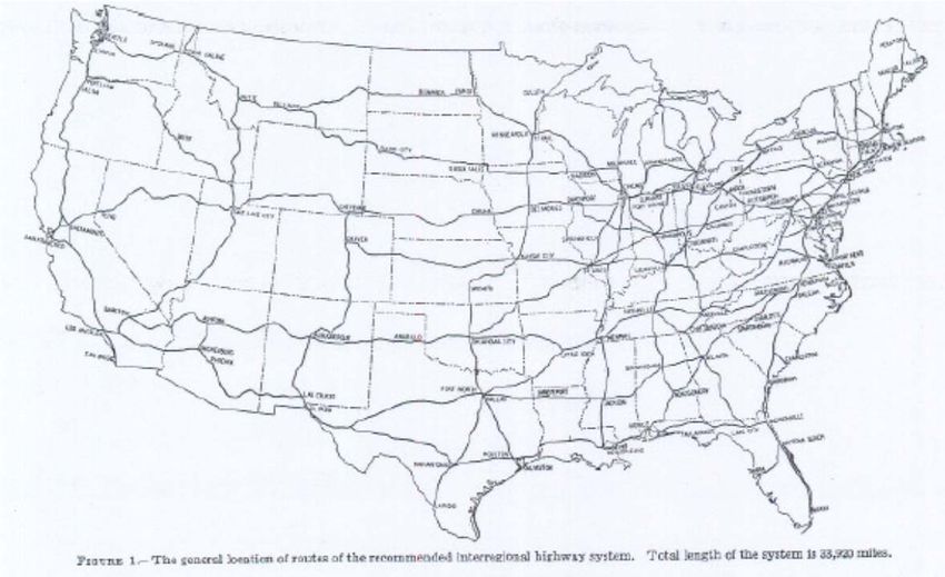
We also construct an alternative instrument based on one of the first proposed maps for the
national interstate highway system. Specifically, we obtained data on the number of proposed
interregional highway miles in each state from the 1944 highway system recommendation put
forth by President Franklin D. Roosevelt’s National Interregional Highway Committee (NIHC).
This plan became the basis for subsequent highway system proposals and was eventually enacted
in the 1956 Interstate Highway Act. Because the cross-state distribution of miles in this original
1944 proposal is highly correlated with the distribution of highway miles (and other road factors)
today, this instrument is a remarkably strong predictor of the cross-state distribution of ARRA
highway grants some 60 years later.
Our results indicate that ARRA highway grants did in fact lead to higher state-
government highway spending than would have occurred in the ARRA’s absence. In particular,
we estimate that each dollar of ARRA grants led to nearly one additional dollar of state highway
spending in 2010, implying little if any crowd-out. This result is extremely robust and holds
across a variety of specifications, including across our two alternative instruments and including
a wide variety of conditioning variables. We also estimate the effect of the ARRA highway
grants on spending in 2009 and 2011. We find a small but statistically significant effect of the
ARRA grants in 2009 and a large and significant effect in 2011, which is consistent with
substantial time lags between grant announcements and outlays. Using Jordà’s (2005) local
projection method, we find that the cumulative effect of grants on highway spending over the
2009-2011 period is roughly two dollars per dollar of grants, suggesting some crowding-in of
states’ own funding for highways, perhaps due to complementarities between road projects
eligible for federal reimbursement and those that are not.
In addition, we document that that the higher state highway spending resulted in
employment increases in sectors most directly affected by highway expenditures, for instance the
road construction sector. In particular, our estimates for 2010 imply that each $1 million of
ARRA highway grants received by a state resulted in approximately 2 additional road
construction jobs. Given that ARRA highway grants totaled about $25 billion nationally, this
implies a national effect of roughly 50,000 jobs, which is equivalent to a 16% increase in road
4construction employment from September 2008. We also detect some modest spillover effects on
employment in sectors most likely to benefit from improved transportation infrastructure.
In our analysis, we pay particular attention to the timing of federal highway grants and
show that our results are also robust to using different accounting measures with different time
lags (for instance, apportionments versus obligations or outlays). This is particularly important
since, depending on the timing, some of these measures can be anticipated, which can alter the
estimated effects on state-government spending (see, Ramey (2011) and Leduc and Wilson
(2013)).5 In particular, federal grant apportionments to states are known first and then obligated
by the states to finance particular projects. However, states are not reimbursed by the federal
government until the projects are completed, and then the federal payments show up as outlays.
Importantly, our estimated effect of roughly dollar-for-dollar spending from grants in 2010 holds
whether we measure ARRA highway grants using data on apportionments, obligations, or
outlays.
Our evidence of a strong effect of ARRA highway grants on highway spending is
particularly striking given that states generally faced no requirement under ARRA to match any
fraction of highway projects’ costs, making the funds fully fungible. In turn, it begs the question
of whether the strong effect of ARRA highway grants reflects some unique characteristics of the
ARRA. To answer this question, we extend our analysis and estimate the effect of highway
grants on state highway spending using an IV panel data model similar to that of Knight (2002)
but with a much longer sample, from 1983 to 2008. While we are able to replicate Knight’s
complete crowd-out result using his one-way (state) fixed effects model and his 1983-1997
sample period, we find that extending the sample period yields an effect of nearly one, on par
with that found in the 2010 cross-section. Our results thus suggest little change in the effect of
highway grants over the past 15 years, contrary to a recent assessment by the CBO (2013).
Our paper also complements the recent empirical work on the effects of ARRA on
economic activity. In general, this literature has documented important employment effects from
ARRA spending using employment variation across time and states, with the estimates differing
somewhat across studies (see, for instance, Wilson (2012), Feyrer and Sacerdote (2011),
Chodorow-Reich et al. (2012), and Conley and Dupor (forthcoming)). The results of this paper
5
Carlino and Inman (2013) develop narrative measures of federal grants-in-aid since the mid-1950s to deal with
anticipation effects associated with this form of federal transfers.
5suggest a possible transmission channel for this effect that would operate through increases in
state spending.6 However, we acknowledge that these results may not generalize to other types of
grants. In this case, the transmission channel may operate through other channels, for instance
via lower state taxes than would be the case absent the additional federal grants. In addition, by
documenting the degree of crowd-out during a deep recession when state governments are under
acute budgetary pressures, our paper fills an important gap in the public finance literature on the
flypaper effect. One exception is the work of Gramlich (1978, 1979), which examines the effects
of different grants in the 1977 economic stimulus program using an estimated model of state and
local governments.
The remainder of the paper is organized as follows. In the next section, we discuss the
importance of grants in the 2009 Recovery Act and the particular requirements attached to the
distribution of highway grants to states. Section III presents our methodology and identification
strategy, while the data are described in Section IV. We then present our main results, followed
by a battery of robustness exercises. Section VI extends our analysis to the period before the
Recovery Act, while the last section concludes.
II. Federal Grants and the American Recovery and Reinvestment Act
The financial crisis in the fall of 2008 and the rapid decline in economic activity that
followed led to the enactment of the American Recovery and Reinvestment Act (ARRA) in early
2009. Initially estimated to cost $787 billion over ten years and subsequently revised upward to
$840 billion, the Act involved a combination of tax cuts, representing roughly one-third of the
total cost of the bill, and increases in expenditures.7 Although the full cost of the legislation is
expected to spread over ten years, an estimated 75 percent of the cost occurred in fiscal years
2009 and 2010.
Federal transfers to state and local governments are a central part of the ARRA. For
instance, the Bureau of Economic Analysis (BEA) reports that between 2009 and 2012, $282
billion was paid out in federal transfers to state and local governments to help support spending
6
Recent preliminary work by Fisher and Wassmer (2013) looks at the closely related issues of how state and local
expenditures on total public capital (of which roads are a subset) has varied over the 2000-2010 period and whether
ARRA highway grants helped mitigate cuts in public capital expenditures during 2009 and 2010. Consistent with
the results in this paper, their OLS panel fixed effects regressions indicate a large positive effect of these grants on
state and local public capital spending.
7
Recovery.gov provides updates on the breakdown of the ARRA’s cost
(http://www.recovery.gov/Transparency/fundingoverview/Pages/fundingbreakdown.aspx)
6on health, education, infrastructure, and other programs, representing over half of ARRA outlays
during this period. Capital grants for transportation infrastructure constituted nearly $50 billion
of these transfers between 2009 and 2012, with $27 billion going to the financing of highway
infrastructure projects.
To speed up disbursement, the Recovery Act was designed to channel the majority of funds
to states via existing transportation programs. For instance, the ARRA highway funds were
partly distributed to states according to the apportionment mechanism corresponding to the long-
standing Surface Transportation Program under the umbrella of the Federal-Aid Highway
Program through which federal highway grants have historically been apportioned to states.8 As
a result, state transportation officials had a good understanding of project eligibility and other
federal requirements, which facilitated the timely distribution of federal grants.
The desire to expedite the disbursements of highway grants led legislators to include
additional requirements in the ARRA that are absent from the procedures used to apportion
typical (non-ARRA) federal highway funds. In particular, the Recovery Act included much
shorter deadlines to obligate the funds apportioned to the states. 9 Compared to the normal four
years, the ARRA stipulated that states had a maximum of 18 months to obligate the funds from
the date of apportionment. Thus, funds apportioned in early 2009 needed to be obligated by
September 30, 2010. Apportioned funds not obligated within this time frame were to be
rescinded. In addition, highway projects that could be completed (i.e., expenditures fully outlaid)
within three years were to be given priority.
These timing requirements had a clear impact on the types of projects that states financed
with the stimulus funds. For instance, the Government Accounting Office (GAO) (2011)
reported that, as of June 2011, 68 percent of obligated ARRA highway funds had been used to
finance pavement-related highway projects: resurfacing, reconstruction or widening of existing
highways. In contrast, new highway construction projects represented only 7 percent of the
obligated funds. (An example of a new infrastructure project financed with ARRA grants is the
expansion of the Caldecott Tunnel on Highway 24 near Berkeley, CA).
8
See Leduc and Wilson (2013) for a comprehensive view of the Federal-Aid Highway Program.
9
As we describe later, federal funds are first apportioned to states using formulas. Once a project is approved by the
relevant federal oversight agency for financing, states then obligate the federal funds, which legally binds the U.S.
government to repay the states for the cost of the project.
7The Recovery Act also included maintenance-of-effort (MOE) requirements. 10 This
provision specified that the governor of each state needed to certify that the state would maintain
its planned level of transportation spending from February 2009 through September 2010. The
goal of the requirement was to ensure that federal funds would be used to add to, instead of
substitute for, state funds and ultimately raise overall transportation spending.
Observers have doubted the effectiveness of these MOE requirements for a few reasons.
First, the governor certifications were due by March 19, 2009, several weeks after each state
learned how much in highway grants had been apportioned to the state. Though governors were
instructed to base their certification on expenditure plans as of February 17, 2009, when the
Recovery Act passed, there was little if any enforcement mechanism to ensure that states would
not adjust planned expenditures in response to these grant apportionments. 11 Second, it is
difficult for states to precisely forecast their revenue and plan their level of spending in an
unexpectedly deep downturn such as the Great Recession and its aftermath. As budget balances
worsened more beyond expectations over the 2008–2010 period in particular, states faced severe
pressures to reduce spending. Third, the penalty for failing to meet the MOE requirements was
small. A state that failed to meet the MOE requirement for ARRA highway grants was still
eligible to receive all of the originally apportioned funds. However, it would miss out on the
FY2011 redistribution of unobligated funds (from other states that did not fully obligate funds
within the required time frame), which is small compared to total annual state apportionments.12
Finally, the federal government may be hesitant to fully enforce MOE requirements in a
recession because it means decreasing aid to the very states that may need it the most, those
unable to maintain spending levels given unexpected declines in economic activity and tax
revenues.
Finally, the Recovery Act did not require states to share the cost burden of federally
financed highway projects, in contrast to non-ARRA highway grants, which typically call for
10
For details on the MOE requirements for ARRA highway grants, see
http://www.fhwa.dot.gov/economicrecovery/guidance.htm.
11
Moreover, even expenditure plans as of February 17 likely would have anticipated a substantial increase in federal
highway aid as some legislation like the Recovery Act was widely expected in the weeks leading up to its
enactment.
12
At the end of each fiscal year, the federal highway administration reassesses the ability of each state to obligate its
apportioned funds and adjusts the limitation on obligations, decreasing it for some states and increasing it for others.
For instance, for fiscal year 2010, the GAO (2011) reported that $1.3 billion in obligation limitations were available
for redistribution. That was less than 1% of total highway grant obligations in 2010.
8states to cover 20 percent of the costs. Although the absence of matching requirements lowered
the cost to the states of using ARRA highway grants, it also made those grants more fully
fungible, making it more likely that the ARRA funds would crowd out state spending.
The importance of ARRA highway grants relative to non-ARRA grants is shown in Figures
1 to 3. For instance, Figure 1 shows that states received between $50 and $100 (in constant 1997
dollars) per capita in apportioned highway grants annually between 1983 and 2008. The
Recovery Act added over $80 per capita ($27 billion) in 2009 to apportioned highway grants, a
near doubling in a single year. As mentioned above, states generally were required to obligate
these apportioned funds to specific projects by September 30, 2010. Consequently, the
enormous surge in apportionments led to a sharp increase in highway grant obligations over 2009
and 2010 before returning to pre-ARRA levels in 2011, as shown in Figure 2. At first glance,
Figure 2 thus suggests that states did not use ARRA highway grants as a substitute for non-
ARRA. The outlays eventually resulting from these highway grant obligations are shown in
Figure 3. Although the majority of apportioned grants was obligated in 2009, ARRA outlays
rose most in 2010 and continued into 2011. This feature is consistent with the substantial time
lags between apportionments and outlays that are discussed in FHWA (2007) and more precisely
documented in Leduc and Wilson (2013).
III. Methodology
To motivate our main empirical specification, it is useful to start by considering a simple
regression model describing the determination of the level of state highway spending per capita
in some post-ARRA year (t) in state i. We model this level as a linear function of highway
grants ( ), a vector of conditioning variables ( ), a time-invariant state fixed effect ( ), and a
time fixed effect ( ):
(1)
The coefficient of interest is , which captures the effect of highway grants on state government
highway spending. Hereafter, we adopt the terminology of the public finance literature and refer
to this effect as the “flypaper effect.” Under the hypotheses that the grants are completely
fungible and state governments are rational and benevolent, one should expect a flypaper effect
far below one ( ). In particular, if roads are a normal good, then should be equal to roads’
share of total state government expenditures, which averaged 0.065 in 2010. A flypaper effect
9above this level would thus indicate less than perfect crowd-out of a state’s own highway
funding in response to highway grants.
An obvious concern with this level specification is that unobserved state fixed effects,
such as time-invariant geographical or climatic characteristics, may cause bias even in the
instrumental variables/generalized method of moments (IV/GMM) regressions if these fixed
effects are correlated with both state highway spending (conditional on controls) and the
instruments. For instance, geographically large states with spread-out populations tend to have
high values of interstate miles per capita and other road-related formula factors and hence
receive comparatively large amounts of highway grants per capita. And because their population
is spread out, they arguably would spend large amounts per capita on roads even without the
federal grants.
One can remove these fixed effects by time-differencing equation (1) ,
(2)
where denotes the J-year difference operator.
While time-invariant state characteristics may influence the level of state highway
spending, there is little reason to think they should affect the change in state highway spending.
In fact, as a robustness check below, we condition on the state’s trend (i.e., change) in highway
spending per capita over the ten years before ARRA and find that it is economically and
statistically insignificant and that its inclusion has very little effect on grants’ estimated effect on
spending. Because our concern is with estimating the effect of the ARRA highway grants on
post-ARRA highway spending for years , we take differences with respect to 2008
values. Specifically, when , we take a one-year difference; when , we take a
two-year difference; and when , we take a three-year difference.
In some specifications below, we measure using total (ARRA and non-ARRA)
highway grants. However, because the primary focus of the paper is on estimating the flypaper
effect of ARRA highway grants, generally we will use only ARRA highway grants, which we
denote here as . Notice that in this case, the estimating equation becomes
(3)
The second line of the equation substitutes in the identity , which reflects
the fact that for all . That is, ARRA highway grants are, by definition, zero
10before the ARRA’s enactment in 2009. Thus, if the time-difference is t relative to 2008 or any
other pre-ARRA year, then the difference in ARRA grants is simply the level of grants in year t.
Our baseline results are based on estimating equations (2) and (3), using both OLS and
IV/GMM. There are two primary endogeneity concerns. First, states with more lane-miles per
capita and other road-related formula factors may also coincidentally have been hit harder by the
recession and/or recovered faster after the recession, leading to a spurious correlation between
ARRA highway grants (and formula factors) and post-ARRA state highway spending. For
instance, less dense states with more lane-miles per capita may have had steeper house price run-
ups prior to the recession, larger housing crashes in the recession, and then sharper housing
recoveries in 2009-2011 at the same time that they received more ARRA highway grants. We
address such concerns via selection-on-observables. That is, we condition on a number of
variables likely to capture pre-ARRA trends in state highway spending, state house prices, and
overall state economic conditions, as well as variables capturing the political environment of the
state.
A second endogeneity concern is that, while most ARRA highway grants were
distributed according to the pre-existing formulas described earlier, some portion may have been
distributed in an endogenous manner. For instance, the Department of Transportation may have
been influenced by political pressure to direct funds disproportionately to politically powerful
states (particularly if politically powerful states were also states that would have increased road
spending relative to other states even in absence of ARRA) or may have wanted to direct funds
disproportionately to states perceived to be more in need.
We address this concern via instrumental variables. We use two alternative sets of
instruments. The first set consists of the state’s number of interstate highway lane-miles and the
state’s contributions to the Highway Trust Fund (HTF) attributable to commercial vehicles.
These two variables are a subset of the road-related factors used in the statutory formulas for
apportioning the bulk of federal highway grants to states. These formulas have been used for
several decades in the multiyear federal highway authorization acts. In writing the legislation on
highway grants in the ARRA, Congress piggy-backed on these pre-existing formulas by
apportioning half of the $27.5 billion in ARRA highway grants in proportion to each state’s
share of overall Federal-Aid Highway Program (FAHP) grants in 2008 and the other half
according to the pre-existing formula used by the Surface Transportation Program (STP), which
11is a subset of the FAHP. The STP formula is a weighted average of a state’s federal-aid highway
lane-miles (0.25 weight), vehicle-miles traveled (0.40), and contributions to the HTF (0.35). The
formulas for the other major programs in the FAHP, the Interstate Maintenance (IM) and the
National Highway System (NHS), use very similar factors. For instance, the IM formula is an
equal-weighted average of interstate vehicle-miles traveled, interstate lane-miles, and
contributions to the HTF attributable to commercial vehicles.
For all FAHP programs, grants for a given year are apportioned based on data for these
factors as of three years prior. The three-year lag is due to lengthy lags involved with collecting
and processing the data. In particular, the 2009 ARRA grants were apportioned as functions of
road factors from 2005 (for the half of funds using 2008 FAHP apportionment shares) and 2006
(for the half based on STP’s formula). Because we are using these factors as instruments for a
given year’s grants, the three-year lag fortunately further ensures the exogeneity of these factors
with respect to a state’s current economic activity and its current highway spending decisions. In
our baseline specifications, we use just the measures of interstate lane-miles and HTF
contributions used in the IM formula as instruments rather than the full dozen or so road factors
going into FAHP formulas, to avoid potential biases from using a large number of instruments
(see, e.g., Hansen, Hausman, and Newey (2008)). Using the full set yields little additional first-
stage power given that the road factors tend to be highly correlated. We also exclude vehicle-
miles traveled as an instrument because it is possible that this variable (even with the three-year
lag) is correlated with contemporaneous economic activity. That said, the results are quite robust
to including additional road factors as instruments.
The second instrument set consists of the number of highway miles in each state
according to the original 1944 proposal for the interstate highway system put forth by President
Franklin D. Roosevelt’s National Interregional Highway Committee (NIHC). The 1944 NIHC
report contained both a map and a table indicating the number of proposed highway miles by
state corresponding to the committee’s recommendation for a new national interregional
highway network. The map is shown in Figure 4 below.13
13
This map also was used as an instrument for county-level rural highway construction in Michaels’s (2008) study
of the labor market effects of reduced trade barriers.
12Figure 4. Map of Proposed National Highway System in 1944 NIHC Report
The 1944 plan became the basis for interstate highway system proposals, including the
1947 map used to construct city-level instruments in the studies of Baum-Snow (2007) and
Duranton and Turner (2011, 2012), as well as for the actual 1956 Interstate Highway Act, which
initiated the construction of the U.S. interstate highway system as we know it today. Because
modern spending on the interstate highways has consisted largely of widening, improving, and
adding lanes to the original highways rather than building new routes, the initial 1944 plan is
highly correlated with the geographic distribution of highway lane-miles today. Furthermore,
because modern-day lane-miles, as well as other strongly correlated road factors were used to
determine the apportionment of ARRA highway grants to states, there arises a rather remarkable
positive correlation between the 1944 highway network and the cross-state distribution of ARRA
highway funds some 65 years later. Indeed, as the ARRA funds account for the bulk of the
increase in total federal highway funds from 2008 to 2009, there also turns out to be a positive
correlation between the distribution of highway miles in the 1944 plan and the 2008-2009
change in total FHWA grants – a correlation not found in previous year’s changes in grants,
which are functions of changes in road factors as opposed to levels.
13We also report results where we replace these road-related instruments with instruments
measuring each state’s political power in Congress, both in general and on the key committees in
charge of transportation funding. Such instruments were used in Knight’s (2002) study of the
flypaper effect of highway grants over 1983-1997 as well as by the Feyrer and Sacerdote (2012)
study of the employment effects of the ARRA. Consistent with the first-stage results reported in
these other studies, we find the Congressional power instruments are only weakly predictive of
highway grants, both for ARRA years and earlier. Given that IV estimates based on weak
instruments are prone to finite-sample bias (see, e.g., Stock, Wright and Yogo (2002)), we prefer
the regressions using road-related formula factors or the 1944 highway network as instruments.
Nonetheless, as shown below, we obtain very similar results using these Congressional power
instruments.
IV. Data
This section describes the data on state government spending, regular federal-aid
highway grants, ARRA highway grants, the instruments, and the conditioning variables used to
estimate the regressions discussed earlier. Summary statistics for these variables are provided in
Table 1. The statistics are given for the year 2010, except where otherwise indicated, because the
effect of the ARRA highway grants on state highway spending in 2010 is the primary focus of
this paper. All dollar variables are measured in constant 1997 dollars. 14 Our primary sample
includes 48 states. Alaska is excluded because, due to its extreme weather and population
sparsity, it is a major outlier in terms of per capita highway grants and spending. Nonetheless, we
show in a robustness check that the estimated flypaper effect of ARRA grants is even larger
when Alaska is included. Nebraska is excluded because it does not have a bicameral legislature
making two of the conditioning variables (Democrat share of state house and state senate)
undefined. Including Nebraska and dropping those two conditioning variables has virtually no
effect on the results.
A. State Government Spending
14
We use 1997 dollars to deflate variables to facilitate our replication of, and comparisons to, the Knight (2002)
results, as in Table 9.
14Data on highway-related expenditures and total general-fund expenditures by each state
government come from the Census Bureau’s Survey of State Government Finances (SGF). These
data are available from 1977 to 2011. We measure highway expenditures as the sum of regular
and toll highway expenditures on (1) current operations, (2) construction outlays, (3) other
capital outlays, and (4) transfers to local governments for roads. The SGF defines highway
expenditures as expenditures on “[m]aintenance, operation, repair, and construction of highways,
streets, roads, alleys, sidewalks, bridges, tunnels, ferry boats, viaducts, and related non-toll [and
toll] structures.” For each state, data in the SGF are reported for that state’s fiscal year. All but
four states have fiscal years ending June 30 of the named year (e.g., FY2012 begins July 1, 2011
and ends June 30, 2012). The other four states – Alabama, Michigan, New York, and Texas –
have fiscal years ending September 30 of the named year.
B. Regular (Non-ARRA) Federal-Aid Highway Grants
When referring to federal aid, the term “grants” typically denotes the amount of
intergovernmental transfers from the federal government to other levels of government. Yet there
are at least three distinct concepts, or measures, of grants that differ importantly in their timing:
Apportionments, Obligations, and Outlays. These concepts are described briefly below; see
FHWA (2007) for details.
“Apportionments” are the amounts of Congressionally authorized federal funding that
each state is eligible to receive for reimbursement of FHWA-approved highway costs. For
federal highway grants, each program within the Federal Aid Highway Program apportions these
authorized national totals to states based on a statutory apportionment formula, as discussed
earlier. Each year, the annual apportionments for each program are announced at the start of the
federal fiscal year (October 1). At that time, no actual funds are transferred from the federal
government to states. Rather, these announcements inform states of the funding they are eligible
to receive as reimbursement for expenditures on FHWA-approved projects. After states are
informed of their apportionments, they then are able to obligate those prospective funds to
specific FHWA-approved projects. For regular (non-ARRA) highway grants, states typically
have up to four years to obligate apportioned funds. In contrast, an important feature of ARRA
highway grants was the requirement that states obligate funds within 18 months of
apportionment – that is, by September 30, 2010, 18 months from March 2, 2009, the date on
15which ARRA highway grant apportionments were announced (see FHWA (2009)). As
mentioned earlier, this provision was included in the ARRA to provide incentives to states to
start highway projects quickly, while they could provide the greatest countercyclical stimulus,
rather than over the usual several-year process. We provide evidence suggesting that indeed the
lag between grant apportionments and obligations, and in turn outlays, was much shorter for
ARRA grants than for regular, non-ARRA grants.
The sum of state government obligations within each state and year are the FHWA’s
“obligations” for that state-year. These obligations are effectively promises by the federal
government to reimburse the states for future costs. Still, no actual funds are transferred at this
time. Once projects commence and costs are incurred, payments are made from the state
government to the contractors or local government agencies engaged in the work and the federal
government transfers funds to the state government’s general fund. These federal
reimbursements are referred to as FHWA “outlays.”
Data on apportionments, obligations, and outlays are available from the Office of
Highway Policy Information’s annual Highway Statistic Series publications (Tables FA-4, FA-
4B, and FA-3, respectively). For 2009 onward, the reported totals for obligations in these
statistics include FHWA obligations of ARRA funds, while the totals for apportionments and
outlays do not. Data on ARRA FHWA apportionments, obligations, and outlays are available
separately, allowing us to measure these three variables both gross and net of ARRA grants.
C. ARRA Highway Grants
Data on ARRA highway grant apportionments come from the March 2, 2009 FHWA
Notice, “Apportionment of Highway Infrastructure Investment Funds Pursuant to the American
Recovery and Reinvestment Act of 2009, Public Law Number 111-5” (FHWA 2009). Data on
ARRA obligations and outlays by state are available from recovery.gov, the website set up by
the federal government to provide information to the public about how ARRA funds are being
spent. For each government department, the website provides weekly Financial and Activity
Reports containing the cumulative-to-date amounts of awards and outlays for each specific grant,
loan, or contract by state and subagency (such as the FHWA). From the Department of
Transportation’s Financial and Activity Reports, we computed the sum of all FHWA-issued
16grants – measured by both obligations and outlays – by state over the course of each federal
fiscal year (2009-2011). (FHWA grants are identified by the TAFS code 69-0504.)
In our cross-sectional regressions, which focus on the effect of ARRA grants on state
government highway spending in 2010, we consider three alternative measures of ARRA
highway grants. The first is ARRA highway apportionments to the state (i.e., the announcements
of ARRA highway grant apportionments on March 2, 2009). The second is the ARRA highway
obligations through the end of the federal fiscal year 2010 (September 30, 2010). This variable
turns out to be nearly equivalent to ARRA highway apportionments because of the ARRA
requirement that apportioned funds be obligated within 18 months of the apportionment date –
that is, by September 2, 2010. The third measure is ARRA highway outlays through the end of
(federal) fiscal year 2010. In some regressions, we look at state government highway spending in
2011; for those regressions, we use ARRA highway apportionments, obligations, and outlays
through fiscal year 2011, though ARRA apportionments were zero after 2009 and obligations
were very close to zero after 2010.
It is worth noting that there is a one-quarter misalignment between our data on state
government spending and federal grants. Four states (Alabama, Michigan, New York, and
Texas) have the same fiscal year as the federal government, which ends September 30 of the
calendar year. But the other 43 states in our sample have fiscal years that end one quarter earlier.
This misalignment can be thought of as adding measurement error to the true dependent variable,
state government spending within the federal fiscal year. As long as this measurement error is
uncorrelated with highway grants (for ordinary least squares (OLS) regressions) or with the
instruments (for IV regressions), it will not cause any bias and will be reflected in the size of the
standard errors.
D. Instruments
Data on FHWA apportionment formula factors comes from the Office of Highway Policy
Information’s annual Highway Statistic Series publications, Table FA-4E. The number of miles
in each state of the 1944 NIHC proposed national highway system can be found in Table 1 of the
1944 NIHC Report to Congress (NIHC 1944, pp. 8-9). The Congressional power instruments
used in some specification came from Stewart and Woon (2012).
17E. Conditioning Variables
Our baseline specification includes several conditioning variables that could potentially
affect or predict post-ARRA state highway spending while also being correlated with ARRA
highway grants or the instruments. We include the 2008-2010 change in state income per capita
(in 1997 dollars), using data from the Bureau of Economic Analysis. We also include the 2008-
2010 change in three variables meant to capture the state’s residents’ preferences regarding
public spending. These variables were also included in Knight’s (2002) study of the flypaper
effect of federal highway grants. The first is an indicator variable for whether the governor is a
Democrat (1) or Republican (0). The other two are the share of legislators in the state’s House of
Representatives that are Democrats and share of legislators in the state’s Senate that are
Democrats. The data for these political variables come from the Council of State Governments.
In various robustness checks presented later in the paper, we also condition on a lagged
dependent variable (2006 to 2008 change in highway spending), the ten-year trend in highway
spending leading up to the Recovery Act, the pre-recession run-up in house prices, the 2008 level
of the index of leading economic indicators (from the Federal Reserve Bank of Philadelphia), the
2006 to 2008 change in the index of leading indicators, and the 2008 levels of the three political
variables described above.
V. Results
A. OLS
The results from estimating variations on equation (3) via Ordinary Least Squares are
shown in Table 2. Identification in the OLS case is based on the selection-on-observables
assumption, which posits that, conditional on the observed covariates, the amount of ARRA
highway grants received by a state is uncorrelated with the residual of state highway spending (
in equation (3)). The dependent variable in each regression is the 2008-2010 change in state
highway spending per capita. The regression in the first column includes only a constant along
with the level of 2009 ARRA highway grant apportionments.15 Column (2) adds changes in the
political preferences variables, and column (3) adds the 2008-2010 change in income per capita.
15
All three measures of ARRA highway grants in Table 2 and subsequent tables are cumulative amounts through
the end of fiscal year t (where t is 2009, 2010, or 2011, matching the end‐year of the dependent variable). For
ARRA highway apportionments, this cumulative measure is constant over t because the entirety of ARRA highway
grants were apportioned in 2009.
18The coefficient on grant apportionments is very similar, about 0.7, across the three cases and is
highly statistically significant – both relative to zero and relative to the share of highway
spending in total spending, which as mentioned earlier averages about 0.07. The coefficients in
columns (1) and (3) are not statistically significantly different from one, while the coefficient in
column (2) is significantly different from one at the 10% level. Columns (4) and (5) repeat the
regression in Column (3) but with alternative measures of ARRA highway grants. Using
cumulative ARRA FHWA obligations through the end of fiscal year 2010 (column (4)) yields
nearly identical results. Using cumulative ARRA FHWA outlays (column (5)) yields a somewhat
larger effect of about 0.9. The coefficient on obligations is statistically significantly different
from one (at the 5% level) while the coefficient on outlays is not significantly different from one.
Recall that a coefficient near zero (near highway’s typical share of total state spending)
would indicate that federal grant funds are entirely fungible – treated by states no differently than
any other general revenue. In contrast, a coefficient of one implies a perfect flypaper effect,
whereby each additional dollar of federal highway grants leads to an additional dollar in highway
spending by the state government. A coefficient above one would imply that federal highway
grants not only cause a dollar-for-dollar increase in state highway spending but also crowd-in
additional highway expenditures by the state. Thus, the OLS results strongly reject complete
fungibility and instead indicate a very strong flypaper effect.
B. First Stage of IV/GMM – Exogenous Determinants of ARRA Highway Grants
As mentioned earlier, one possible concern about the OLS results is that the distribution
among states of some portion of the ARRA highway grants could have been endogenous with
respect to post-ARRA highway spending. We address this concern via instrumental variables.
Before presenting the IV/GMM second-stage results, which give estimates of the flypaper effect
of ARRA highway grants on state government highway spending, we evaluate the strength and
validity of the instruments. We consider the two alternative sets of instruments described in
Section III, the first consisting of road-related apportionment formula factors and the second
consisting of the 1944 NIHC planned highway miles per capita.
The results of the first-stage regression of ARRA highway grants, for each of the three
grants measures, on each set of (excluded) instruments and conditioning variables (included
instruments) are shown in Table 3. The regressions in columns 1, 3, and 5 use 2006 interstate
19lane-miles and 2006 payments to the Highway Trust Fund (HTF) attributable to commercial
vehicles as the excluded instruments. The regressions underlying columns 2, 4, and 6 use the
proposed highway miles in each state according to the 1944 NIHC recommendation. (We
measure this variable on a logarithmic scale to reduce the influence of a few outliers, yielding a
more even distribution and a stronger first-stage fit). Along with coefficients and
heteroskedasticity-robust standard errors, the table also reports the first-stage F statistics and the
p-values on the Hansen-J overidentifying restrictions test (for those regressions containing more
than one excluded instrument). The overidentifying restrictions tests are based on the residuals
from the differences specification (Columns 1-3 of Tables 4 and 5).
The 2006 road factors strongly predict each of the three measures of ARRA highway
grants, as indicated by the very high first-stage F-statistics. Stock and Yogo (2005) provide 5
percent critical values of the first-stage F statistic for the test of weak instrument bias in two-
stage least squares. They find that, for a single endogenous variable and two excluded
instruments, F-statistics above approximately 9 correspond to a bias (of the IV estimator relative
to OLS) of less than 10 percent. The first-stage F statistics on the 2006 road factors are roughly
58. The overidentifying restriction test yields p-values on the null hypothesis of exogeneity that
are well above standard significance levels.
The proposed miles of highways from the 1944 NIHC plan also strongly predict ARRA
highway grants, though not quite as strongly as the 2006 road factors. The first-stage F-statistics
when using the 1944 plan miles range from 29 to 36.
C. Second Stage – The Flypaper Effect
The IV/GMM second-stage results from estimating equation (3) are shown in Tables 4
and 5. The results in Table 4 are based on the 2006 road factors as instruments, while the results
in Table 5 are based on the 1944 NIHC proposed miles. The estimated highway spending effect
of ARRA highway grants, for each of the three grants measures, are shown in columns 1 to 3 of
each table.
Starting with Table 4, we find a very strong flypaper effect irrespective of the grants
measures used. The point estimates in columns 1 to 3 indicate a flypaper effect of ARRA
highway grants on 2010 highway spending of approximately 0.76. In all three cases, the effect is
statistically very far from zero and from highway’s typical share of highway spending (0.065 on
20average); it is significantly different from one at the 5% level. The flypaper coefficient is quite
precisely estimated in large part because of the very strong first-stage fit.
One possible concern with these regressions is that ARRA highway grants could be
correlated with non-ARRA highway grants, which are omitted from the regression and may
independently affect state highway spending. That is, non-ARRA highway grants may have their
own flypaper effect and may be correlated with ARRA grants, biasing the estimated flypaper
effect on ARRA grants. Thus, in columns 4 to 6, we report the results from estimating the
difference-in-differences specification (equation (3)) where grants are measured using total
(ARRA and non-ARRA) obligations or outlays. For apportionments and obligations, we use the
difference from 2008 to 2009, given that there should be at least a one-year lag between either of
these variables and outlays, as discussed earlier. For outlays, the difference is from 2008 to 2010.
The estimated IV/GMM coefficients on the difference in total highway grants are broadly
similar to those found for ARRA highway grants in that they are economically and statistically
far from zero. The coefficients range from about 0.6 when using obligations to about 1.1 when
using outlays. Thus, there is no indication that the flypaper effect found for the ARRA highway
grants was driven by not accounting for a flypaper effect for non-ARRA grants. This result
should not be too surprising given that, as we showed in Figures 1-3, the change in total FHWA
apportionments or obligations from 2008 to 2009 is accounted for primarily by their ARRA
component; and similarly the change in total FHWA outlays from 2008 to 2010 is accounted for
primarily by ARRA outlays.
The results based on using the 1944 NIHC planned miles as instruments are shown in
Table 5. The results are broadly similar to those of Table 4, though the estimated flypaper effect
of ARRA grants is somewhat larger. Specifically, the coefficient on ARRA highway grants
varies from 0.88 to 0.94, dependent on the measure of ARRA highway grants. The coefficient on
the change in total highway grants ranges from 0.71 to 1.32. In all cases, the coefficients are
statistically significantly different from zero but not from one.16
16
Another way to test whether ARRA highway grants do indeed “stick where they hit” is to look at the effect of the
ARRA grants on highway spending’s share of total state government spending. If ARRA grant funds were treated by
states as being completely fungible, they should have no effect of the share of state government spending going to
highways. Regressing the 2008‐2010 change in highway spending’s share of total state government spending on
log ARRA grants per capita yields positive and significant coefficients, around 0.007, in both OLS and IV and for all
three grant measures. A coefficient of 0.007 implies that having 10 percent higher ARRA grants than another state
21Summarizing our baseline empirical results, we find strong evidence that ARRA highway
grants induced states to increase highway spending over the course of 2009 and 2010.
Specifically, we find that each dollar in ARRA highway grants to a given state led to between 76
and 94 cents of additional highway spending in that state in 2010. Note that this result captures
the effect of ARRA grants on 2010 highway spending alone; to assess the total cumulative
flypaper effect of ARRA highway grants, one must add the effects of the grants on spending in
2009 and 2011 (and, possibly, future years), as we do later in the paper.
D. Robustness Checks and Placebo Regressions
We estimate a number of alternative specifications to assess the robustness of our results
and to test alternative explanations. First, we assess the robustness of the results to alternative
specifications such as excluding the conditional variables, including additional conditioning
variables, or dropping outliers. The results of these robustness checks are shown in the first ten
rows of Table 6. Each cell of the table represents a separate regression, showing the IV/GMM
coefficient and standard error on the measure of ARRA highway grants indicated in the column
heading. The regressions use the 2006 road factors as instruments; using the 1944 planned miles
as instruments yields similarly robust results (i.e., coefficients and standard errors similar to
those in columns 1-3 of Table 5).
The regressions underlying the first row include, along with the baseline set of
conditioning variables (as in columns 1-3 of Table 4), a lagged dependent variable – that is, the
2006 to 2008 change in state highway spending per capita. This regression addresses the concern
that there may be unobserved factors correlated with the 2006 road factors that also affected the
2008 to 2010 change in highway spending. For example, more sparsely populated states with
higher interstate lane-miles per capita coincidentally might have been more exposed to the
housing slump beginning in late 2006 and the subsequent financial crisis and recession, and more
exposed states likely would have had a lower (or more negative) change in highway spending
from 2006 to 2008 as well as potentially from 2008 to 2010. This could lead to a spurious
correlation between lane-miles, one of our instruments, and the 2008 to 2010 change in highway
spending. However, conditioning on the lagged dependent variable – the change in highway
is associated with an increase of about 0.7 percentage point in the state’s highway share of spending between
2008 and 2010.
22You can also read