Paired Stated Preference Methods for Valuing Management of White Pine Blister Rust: Order Effects and Outcome Uncertainty
←
→
Page content transcription
If your browser does not render page correctly, please read the page content below
Journal of Forest Economics, 2020, 35: 75–101

Paired Stated Preference Methods for
Valuing Management of White Pine
Blister Rust: Order Effects and
Outcome Uncertainty
 James R. Meldrum1 , Patricia Champ2 , Craig Bond3 and Anna Schoettle2∗
1
  U.S. Geological Survey, Fort Collins Science Center, 2150 Centre Ave Bldg
C, Fort Collins, CO 80526, USA
2
  USDA Fort Service, Rocky Mountain Research Station, 240 W Prospect Rd.,
Fort Collins, CO 80526, USA
3
  Colorado State University, Department of Agricultural and Resource
Economics, 501 University Ave, Fort Collins, CO 80523, USA

      ABSTRACT
      The literature on nonmarket valuation includes many examples
      of stated and revealed preference comparisons. However, compar-
      isons within stated preference methods are sparse. Specifically, the
      literature provides few examples of pairing both a discrete choice
      experiment (CE) and a contingent valuation (CV) question within a
      single survey. This paper presents results of a nonmarket valuation
      study that employs both methods to elicit public preferences over
      uncertainty of outcomes and over management strategies. The two
      methods were employed to examine public support for the proactive
      management of the invasive pathogen, Cronartium ribicola, that
      causes the lethal disease white pine blister rust in high-elevation
      forests in North America. By addressing three related questions,
      this study finds the following main results: First, both methods
      suggest the importance of presenting outcome uncertainty to re-
      spondents. Second, the results provide no evidence that preferences

   ∗ Correspondence author: James R. Meldrum, jmeldrum@usgs.gov. This work was

supported by the USDA, Economic Research Service (ERS) Program of Research on the
Economics of Invasive Species Management (PREISM); the USDA-Forest Service Rocky
Mountain Research Station; and the Colorado State University Department of Agricultural
and Resource Economics.

ISSN 1104-6899; DOI 10.1561/112.00000510
©2020 J. R. Meldrum, P. Champ, C. Bond and A. Schoettle
Online Appendix Available at
http://dx.doi.org/10.1561/112.00000510_app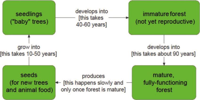
76                                                         James R. Meldrum et al.

      vary over the means taken for pursuing the given ends, which in
      this case is long term forest health. Third, the paired inclusion
      of both methods results in order effects for CE results but not
      for CV results. Results and discussion provide insight into the
      most appropriate stated preference approach for informing different
      types of decisions about the efficient management of public lands.

Keywords: Contingent valuation, Choice experiment, Invasive species, Forest
          management

1    Introduction

Choice experiments (CEs) and contingent valuation (CV) are the two main
stated preference methods for nonmarket valuation (Champ et al., 2017;
Johnston et al., 2017). While both CEs and CV can be structured to ask
precisely the same questions about preferences, the two methods are well
positioned to ask different but complementary questions. CV provides values
for a good, policy, or program. In contrast, CEs provide values for the attributes
that comprise a good, policy, or program. CV is better suited for understanding
public preferences for the entirety of a well-defined program, whereas CEs can
provide “values for changes in a single characteristic or values for changes in
levels of characteristics or values for multiple changes in characteristics . . . ”
(Holmes et al., 2017). These values can be used to provide insight into how
to develop a program based on public preferences. However, compared to
CV, CEs are more cognitively burdensome. Overall, neither method strictly
dominates the other; as Johnston et al. (2017) recommend, “[t]he use of CV or
a CE to describe the change being valued should be based on how respondents
tend to perceive the good, the study objectives, and the information content
of valuation scenarios.” (p. 333)
    The present study asks two different, but closely related, applied questions
relevant to the management of high elevation forests for the disease white pine
blister rust (WPBR), which is caused by the non-native pathogen Cronartium
ribicola. The CV question asks about the overall value of a national-level
program and its success in securing the long-term sustainability of the associ-
ated species, whereas the CE questions seek estimates of marginal values to
support development of efficient management plans and actions. While general
nonmarket benefits from forests are well documented (Barrio and Loureiro,
2010), fewer studies investigate the nonmarket benefits from managing invasive
species in forests (Holmes et al., 2008; Kramer et al., 2003; Rosenberger and
Smith, 1997; Rosenberger et al., 2012).
Paired Stated Preference Methods for Valuing Management... 77
A rich literature assesses the convergent validity of CEs and CV by com-
paring estimated results from the two. The typical approach in this literature
involves implementing the two methods with similar attributes in a split-sample
design, with the CE administered to one sample and the CV to the other.
Some studies using this approach found no significant differences between
the CE and CV values, including in the contexts of solid waste management
decisions (Jin et al., 2006), beach quality improvements (Loomis and Santiago,
2013), land-use management preferences (Dachary-Bernard and Rambonilaza,
2012), and wetland ecosystem service valuations (He et al., 2016). Other
studies found significant differences between CE and CV values between the
split samples. Petrolia et al. (2014) used a split sample to compare a CE
with a “binary choice” CE, functionally equivalent to CV, for valuing restora-
tion of coastal wetlands, and found substantially higher values in the single
referendum-style (i.e., CV) choice. Neher et al. (2018) compared CE and CV
values for white water boating in the Grand Canyon at different hypothetical
flow levels and found a difference in values for one of four flow levels, suggesting
that the difference could result from either a lack of familiarity with that case
or from the functional forms used for estimation. The present study extends
the literature not by directly investigating comparability of results, but rather
by investigating how the nature of the good, policy, or program being valued
and the presence of the other stated preference question in the survey relate
to the CE and CV responses.
Specifically, the present study differs from the typical study in the literature
in that (a) its CE and CV questions are not directly comparable, yet (b) all
respondents faced both types of questions but with the order of the two sets of
questions randomized in a split sample approach. We examine three questions.
RQ1: How does the stated uncertainty of management outcomes affect results
from both methods? RQ2: Do preferences vary over the means taken for
pursuing the given ends, which in this case is long term forest health? RQ3:
Does the paired inclusion of both methods influence responses?
2 Background
Though non-native forest pests and diseases are well recognized to be a
substantial threat to biodiversity and ecosystem services worldwide, rigorous
understanding of the economic and nonmarket effects of many of these invasions
remains elusive (Boyd et al., 2013; Lovett et al., 2016; Aukema et al., 2011;
Holmes et al., 2009; Born et al., 2005). There is sparse understanding of
the nonmarket values associated with limiting the spread of invasive forests
disease. Among the few related studies, Drake and Jones (2017) use CV to
elicit public willingness to pay (WTP) to protect against two specific forest
diseases in England and Wales, and Sheremet et al. (2017) use a CE to find78 James R. Meldrum et al.
significant public benefits to addressing invasive plant diseases more generally
in the UK. The present study expands on the analysis of CV data for the
context of managing WPBR in high elevation, five-needled pine forests that
was previously reported by Meldrum et al. (2011, 2013) and Meldrum (2015).
It also builds on the findings of Naughton et al. (2019), who use a separate
CV study to estimate willingness to pay for managing whitebark pine, one of
the species threatened by WPBR, against multiple threats.
The present survey pairs CV questions aimed at eliciting public prefer-
ences for a national-level program to address this invasive species with CE
questions aimed at eliciting public preferences relevant to the optimization of
landscape-level management plans. One applied question concerns whether
public preferences for WPBR management are affected by the specific types
of management actions taken. Although the pathogen’s complex lifecycle
makes either eradication or containment of the disease unlikely, promising
interventions such as prescribed burning, mechanical thinning, and planting
genetically-resistant five-needled pine seedlings exploit the natural resistance of
some trees to rust to improve these forests’ resilience to the disease (Schoettle
et al., 2018; Jacobi et al., 2017; Schoettle et al., 2014; Burns et al., 2008;
Schoettle and Sniezko, 2007; Samman et al., 2003). Previous CE research in
other contexts has found mixed results on whether program attributes matter
to study participants independently from primary outcomes. For example,
Rolfe and Windle (2013) and Rogers (2013) found evidence that preferences
over conservation outcomes for marine parks in Australia were influenced by
CE attributes describing the management processes used to achieve those
outcomes, whereas McVittie and Moran (2010) found respondents indifferent
among different levels of restrictions in marine conservation zones, holding
conservation outcomes constant. Johnston et al. (2012) found higher value
estimates for indirect effects from restoration projects (e.g., fish-dependent
wildlife species survival) versus direct effects (e.g., increases in the long-run
probability of fish run survival). Closer to the present context, Rossi et al.
(2011) found a preference for replanting over prescribed burning as a policy for
southern pine beetle prevention on private forests, and Sheremet et al. (2017)
found that WTP for forest disease control depends on the control methods
used, with lower support for clear felling and chemicals than for thinning.
To the authors’ knowledge, the literature has yet to implement a paired
stated preference approach to investigate how uncertainty related to manage-
ment outcomes and differing means to the same ends affect the results from the
two valuation approaches. The few examples of paired CE and CV questions
within the same survey tend to be structured so that results are directly
comparable. Adamowicz et al. (1998) estimated separate and joint models of
CV and CE data and found favorable properties from the CE model and either
somewhat lower or somewhat higher welfare measures from CE, depending on
assumptions. Hynes et al. (2011) compared CV results with those from a setPaired Stated Preference Methods for Valuing Management... 79
of CE questions asked later in the survey and found no statistically significant
differences between the CV and CE responses. While these examples do not
consider potential order effects from the multiple question types, Johnston
et al. (2017) suggested that survey design with multiple valuation questions
must consider the impacts of their sequencing. For example, Day and Prades
(2010) and Day et al. (2012) demonstrated implications of ordering in the
sequence of multiple CE questions, and numerous theories from behavioral
economics predict that the order of different questions can influence responses
more generally (Alevy et al., 2011; Carlsson, 2010). In the present study, the
pairing of the two methods allows investigation of not only the relationship of
estimated results, but also how the two instruments might interact.
Complex ecological processes associated with many management interven-
tions result in uncertain outcomes. Management interventions for WPBR in
high-elevation forests fall squarely into this category. The long generation
time of the five-needled pine species that are threatened by WPBR means the
long-run effectiveness of any management plan is uncertain (Burns et al., 2008;
Samman et al., 2003; Schoettle and Sniezko, 2007; Field et al., 2012). Thus,
this study also focuses on the implication of explicitly addressing uncertainty of
management outcomes within both the CE and CV designs. That is, it focuses
on uncertainty not over whether the plan is implemented but rather whether it
is successful. Johnston et al. (2017) pointed out that the literature increasingly
demonstrates the importance of addressing risk and uncertainty in program
outcomes. For example, Roberts et al. (2008) found substantially higher WTP
to avoid algae blooms and maintain normal water levels when they presented
CE choices with uncertainty versus with certainty. They suggest multiple
possible reasons for this counterintuitive result, including that the stated end-
state uncertainty “promotes a more realistic choice . . . and may thereby better
approximate choice behavior in real situations,” that “when the choice question
is more complex, consumers more critically evaluate the tradeoffs between the
attributes that vary among the options,” or that perhaps respondents “may
respond to the [certain] choice questions by assigning subjective probabilities
to the outcomes in the experiment” (p. 592). Wielgus et al. (2009) found that
model fit improved when they explicitly stated a high outcome probability ver-
sus when they provided no information on outcome uncertainty, and Cameron
et al. (2011) described “scenario adjustment” as the effect when participants
may accept a scenario described by a stated preference question yet “ ‘adjust’
some of its informational aspects to fit their own personal situation, history or
context” (p. 10), as Flores and Strong (2007) found for CV choices, which can
be influenced by subjective beliefs about project costs. Similarly, Provencher
et al. (2012) conducted a CV study on Eurasian Watermilfoil (Myriophyllum
spicatum) invasions that affect lake quality and demonstrated the importance
of accounting for subjective expectations in the baseline scenario. Accordingly,
a growing number of studies address outcome uncertainty, either by including80 James R. Meldrum et al.
uncertainty over the entire set of non-cost attributes in a choice (e.g., Rolfe
and Windle, 2015; Wielgus et al., 2009), which corresponds to collinear un-
certainty for different outcome characteristics, or by including uncertainty as
an individual attribute (e.g., Glenk and Colombo, 2011; Rigby et al., 2010;
Veronesi et al., 2014), which is more appropriate when not all attributes (e.g.
thinning or burning current acreage) are uncertain. Other studies (Bartczak
and Meyerhoff, 2013; Lew et al., 2010) have found that CE estimates of WTP
under uncertainty depend on the “baseline” chance of the outcome. However,
most of the above examples are CE studies; to date, outcome uncertainty in
CV studies remains relatively uncommon. Closest analogs tend to appear in
the literatures on respondent uncertainty (e.g., Hanley et al., 2009; Ready
et al., 2010), which model respondents’ uncertainty in their own responses,
and on payment and provision uncertainty, which relate to the uncertainty
of the chosen option being implemented and/or respondents being compelled
to make payment (e.g., Champ et al., 2002; Christantoni and Damigos, 2018;
Mitani and Flores, 2014; Poe et al., 2002).
3 Survey and Methods
Survey data were collected as part of a broader project on the costs and benefits
of managing WPBR in high-elevation forests. As described in more detail
elsewhere (Meldrum et al., 2011, 2013; Meldrum, 2015), the survey instrument
was developed through a series of focus groups, a pretest, and extensive
consultation with natural scientists, closely following recommendations of
Champ et al. (2003). Knowledge Networks, Inc.1 administered the online
survey to a probability-based sample of the general population in the western
United States in June of 2010. Over a period of 11 days, 541 of 895 contacted
individuals completed the survey, for a completion rate of 60%. Probability
weights, based on the inverse probability of selection from the population
and correcting for oversampling of the Mountain region to ensure adequate
coverage, were provided by Knowledge Networks, Inc. and used for all reported
estimates. See Table 1 for demographics of raw sample, weighted sample, and
study population; more details are provided elsewhere (Meldrum et al., 2011,
2013; Meldrum, 2015).
In the analyzed sample, the average respondent was 49 years old, and 53%
were women. One in the three respondents (32%) had earned a bachelor degree,
75% were white, non-Hispanic, and the median reported income was between
$50,000 and $59,999. On a five-point scale ranging from strongly disagree (1)
to strongly agree (5), 75% of respondents agreed (4 or 5) with the statement
1 Any use of trade, firm, or product names is for descriptive purposes only and does not
imply endorsement by the U.S. Government.Paired Stated Preference Methods for Valuing Management... 81
Table 1: Demographics of raw sample, weighted sample, and study population.
Raw Weighted
Variable Sample Sample Populationa
Census division
Mountain (MT, ID, WY, CO, NM, 71% 32% 34%
AZ, UT, NV)
Pacific (WA, OR, CA) 29% 68% 66%
Gender
Male 47% 49% 50%
Female 53% 51% 50%
Age
18-29 16% 23% 24%
30-44 22% 28% 28%
45-59 30% 26% 27%
60+ 31% 22% 22%
Educational Attainment
Less than High School 10% 15% 16%
High School 23% 25% 27%
Some College 35% 31% 31%
Bachelor and beyond 32% 29% 26%
Race/Ethnicity
White, Non-Hispanic 75% 59% 55%
Black, Non-Hispanic 2% 2% 5%
Other, Non-Hispanic 6% 10% 10%
Hispanic 14% 25% 29%
2+ Races, Non-Hispanic 2% 4% 2%
Other Criteria
In a Metropolitan Statistical Area 86% 91% 91%
Number of Respondents/Housing 541 541 27,115,377
Units
a
Statistics derived from U.S. Census Bureau, Current Population Survey, 2007, U.S. Census
Bureau, Population Estimates Program, 2009, and 2006–2008 American Community Survey
3-Year Estimates.
that “protecting five-needled pines from the threat of extinction is important”
whereas only 16% agreed that “people should not intervene in high-elevation
forests.” Although only 31% agreed that “tourism related to high-elevation
forests is important,” more than half (63%) have visited at least one of three
major National Parks (Rocky Mountain, Yellowstone, and Glacier) in the
range of the high-elevation white pines, and 75% expect to visit at least one of
those parks in the future. At the time of publication, data are not available82 James R. Meldrum et al.
from Colorado State University but will be made available upon request to
the corresponding author.
3.1 Experimental Design
The survey implemented a split sample design to randomize the order of the
CV and CE questions within the survey. After introductory material and
general questions about familiarity and experience with high-elevation white
pine forests, half of the sample faced two CV questions followed by a series of
six CE choice sets, whereas the other half faced the six CE choice sets followed
by the two CV questions. Both groups were informed of the total number
of questions and the two types of questions prior to being asked to complete
the CE or CV questions. The online survey format assures adherence to the
intended survey order, because the entire survey could not be previewed, and
previous answers could not be revisited after viewing following questions.
The CV experiment consisted of two questions, both of which asked about
a “national-level program that might be used to managed all of the high-
elevation forests in the Western United States”: one without mention of
outcome uncertainty, and a second with explicit inclusion of a projected
outcome uncertainty level. Specifically, question 1 (Q1) asked:
Suppose managers treat [QUANT]% of the high-elevation forests in
the Western United States. As a result, these acres will be healthy
in 100 years from now. The remainder of the acreage would not be
treated. Would your household be willing to pay a one time cost of
$[BID1] to fund this program?
and question 2 (Q2) asked:
Now suppose the managers treat [QUANT]% of the high-elevation
forests in the Western United States, and as a result of these actions,
there is a [UNCRT]% chance that these acres will be healthy in 100
years from now. The remainder of the acreage would not be treated.
Would your household be willing to pay a one time cost of $[BID2]
to fund this program?
where the variables (BID1, QUANT, and UNCRT) were randomly selected
from the set shown in Table 2, and BID2 was randomly selected if the response
to Q1 = “yes” and randomly selected such that BID2 < BID1 if the response to
Q1 = “no.” Note that this constraint introduces a potential downward bias if
the Roberts et al. (2008) result of stated uncertainty leading to higher estimated
values holds. However, whereas the Roberts et al. result was obtained from a
split sample, the present design of consecutive questions required the constraint
to avoid a strictly dominated sequence of questioning in which a “no” responsePaired Stated Preference Methods for Valuing Management... 83
Table 2: Contingent Valuation (CV) Design.
Contingent Valuation (CV) Design
Question 1 Question 2
Cost of program (BID) $10, $25, $50, $100, $1, $10, $25, $50, $100,
$250, $500, $1000 $250, $500, $1000
Portion of forest (QUANT) 30%, 50%, 70% 30%, 50%, 70%
Chance healthy (UNCRT) 100% (implicit) 40%, 65%, 90%
to BID1 is followed by a BID2 > BID1, paired with a lesser (in terms of a lower
chance of long term healthy) but more expensive program. Sensitivity to this
potential bias is investigated below by splitting results to Q2 by response to Q1.
The CE asked respondents to make tradeoffs among long term effectiveness,
costs, and short-term attributes of different management plans in an unnamed
1000-acre forest located on public land in the mountains of central Colorado.
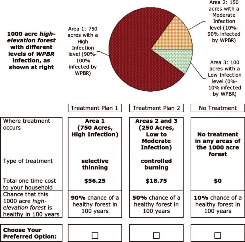
Figure 1 depicts the format of the CE questions. There were two versions of
the CE, based on whether the top panel described the unnamed 1000-acre
forest as having either a “high” or “low” overall current level of WPBR infection.
The “high infection” version (Forest = 1) described a 1000-acre forest that had
750 acres with a high infection level, 150 acres with a moderate infection level,
and 100 acres with a low infection level; the “low infection version” (Forest =
0) described a 1000-acre forest that had 750 acres with a low infection level,
150 acres with a moderate infection level, and 100 acres with a high infection
level. These two versions were included to test whether preferences towards
management and outcomes were dependent on the initial state of the forest;
that is, do preferences for long-term outcomes (ends) depend on what type of
forest is treated (means) (RQ2). Each respondent received only one of the two
versions.
The lower panel of each CE question described three management options
in terms of the attributes shown in Table 3. All attributes, levels, and choice
descriptions were developed with extensive input from natural scientist experts
on WPBR and high elevation forests and with insights gathered through
general-public focus groups. Options were described by where treatment
occurs (referring to the areas described in words and the pie chart in the top
panel), the type of treatment that would be implemented (selective thinning,
controlled burning, planting five-needled pine seedlings that are resistant to
WPBR, or combinations thereof), the total one time household cost of the
program (determined by multiplying one of three cost-per-acre values by the
number of acres treated), and the chance that this 1000 acre high-elevation
forest will be healthy, “defined as natural continuation of all four stages of the
life cycle [depicted in Figure 2] (including forest regeneration) in 100 years”.84 James R. Meldrum et al.
Figure 1: Example of a typical choice set.
The survey instrument (presented in the Online Appendix) also presents
numerous other characteristics of a “healthy” forest, most notably in describing
associated ecosystem services such habitat provision, soil protection, unique
aesthetics, water provision, scientific value, and recreation opportunities.
In addition, each question contained a “no treatment” (status quo) plan
in which no areas of the 1000 acre forest would be treated at a cost of $0,
with an either 10% or 25% baseline chance of this forest being healthy in
100 years without treatment. The baseline chance was held constant for each
respondent but varied independently of the “high infection” or “low infection”
current forest condition (Status quo chance healthy = 0 if 10%, = 1 if 25%).
This was done to test the sensitivity of the results to changes in threat level.
Attribute levels were chosen using a fractional factorial design of six differentPaired Stated Preference Methods for Valuing Management... 85
Table 3: Choice Experiment (CE) Design.
Choice Experiment (CE) Design
Status Quo Alternatives
Cost per Acre $0 $0.05, $0.075, $0.10
Acres treated 0 100, 250, 750, 900, 1000
Treatment type n/a Thin, Burn, Plant, Thin &
Plant, Burn & Plant
Chance healthy 10%, 25% 50%, 70%, 90%
Figure 2: Schematic depicting life-cycle of five-needle pines in a healthy high-elevation forest.
blocks of six choice sets, selected to minimize the D-efficiency criteria (Lusk
and Norwood, 2005).
To summarize, the study involved three treatments (Status quo chance of
healthy, Forest, and Order), each of which was implemented via a split sample.
As depicted in Figure 3, these three treatments address this study’s three
primary research questions. Split samples were balanced across treatments,
with the three-way combination of treatments generating eight treatment
groups of equal size. Further, RQ1 is also tested by the “chance healthy”
variable within the second CV question and the “chance healthy” alternatives
in the CE questions themselves, and RQ2 is tested by the “treatment type
alternatives” within the CE questions.
3.2 Estimation
CV and CE data are modeled separately. CV results are estimated with a
seemingly unrelated bivariate probit regression with Huber/White/sandwich
estimator robust standard errors, as described in Greene (2012), with controls
for order treatment effects. This approach models the likelihood of each
response (y1 = 1 if answer to Q1 = “yes”, y1 = 0 otherwise, and likewise for y286 James R. Meldrum et al.
Figure 3: Schematic depicting treatment-level research design.
and Q2) as a probit regression of indirect utility, assumed linear in parameters,
with potentially correlated error terms between responses to Q1 and Q2. This
approach contrasts with typical interval-based approaches to estimation of
double-bounded dichotomous choice CV data (Hanemann et al., 1991), because
the introduction of the uncertainty in the follow-up question potentially changes
the hypothetical good, policy, or program being purchased in the question, but
it follows other examples in the literature with two sequential CV questions
(Kramer et al., 2003). Mean WTP is estimated at the mean level of included
covariates following Hanemann (1989), and confidence intervals for all WTP
value estimates were estimated using the Krinsky and Robb (1986) simulation
method with 50,000 replications. Note that this approach allows for negative
WTP estimates, which could be observed if non-pecuniary costs of management,
such as human interference in wilderness-like areas, are associated with greater
disamenity than any benefits of treatment.
Following standard practice (Holmes et al., 2017), CE responses are linked
to the theoretical construct of utility using the conditional logit model in a
random utility framework (McFadden, 1974), in which unobservable utility
is the sum of observable, indirect utility, linear in parameters, and a random
error component with an extreme value type I (Gumbel) distribution. For
modeling, “treatment types” are interacted with the number of acres treated,
the number of “acres treated” are estimated as continuous variable, and the
“total cost” is calculated by multiplying cost per acre by the number of acres
treated. As described below, models are estimated with and without a constant
term (constant = 1 if not status quo), and with and without controls for the
three treatments. Given the known limitations of the conditional logit model,
as well as the heterogeneity demonstrated in previous analyses of the first CV
question, estimation of all models with a mixed logit specification (e.g., Revelt
and Train, 1998) was explored but is not shown below, because estimated
parameter standard deviations were nearly all insignificant, suggesting little
improvement in explanatory value. Mean marginal WTP is estimated as the
ratio of the relevant coefficient to the coefficient for total cost, with confidencePaired Stated Preference Methods for Valuing Management... 87
intervals for all WTP value estimates estimated using the Krinsky and Robb
(1986) simulation method with 50,000 replications. This again allows the
possibility of negative WTP estimates.
4 Results
4.1 Contingent Valuation
Basic CV results and their heterogeneity have been investigated previously
(Meldrum et al., 2011, 2013; Meldrum, 2015). This analysis focuses instead
on introducing the second CV question, which explicitly describes outcome
uncertainty (RQ1), and investigating the potential for order effects between
the CE and CV experiments through the “order” treatment control variable
(RQ3). Main results are shown in Table 4 below. The first column presents
results for a standard probit model of Q1, which ignores uncertainty, and
the second column presents results for the bivariate probit model of both Q1
and Q2.
Estimated results are consistent for Q1 across the first two columns, and
ρ is positive and significant for the bivariate probit, demonstrating a strong
correlation in response across the two questions. Despite previous analyses
teasing out substantial insight from modeling of Q1 alone, Q2, which makes
uncertainty explicit, produces much more nuanced results, suggesting that
respondents attended more fully to the details of the question when presented
with the more realistic outcome-uncertain scenario. While basic cost sensitivity
(i.e. a negative and significant response to the cost of the program) is robust
across questions, a positive response to increasing the portion of forest treated
and chance of long-run forest health is only demonstrated in Q2. This result is
consistent with Roberts et al.’s (2008) suggestion that their similar results stem
from respondents more critically evaluating tradeoffs when a choice question
is made more complex by including end-state uncertainty. The insignificant
coefficients on the Order indicator variable suggest no observable order effects
in the CV question from respondents who faced the CE questions before the
CV questions. Finally, to investigate the potential bias from constraining BID2
< BID1 when Q1 = “no,” the third and fourth columns of Table 4 present
results for a standard probit model of Q2 for the sub-sample answering “yes”
or “no” to Q1, respectively. The final column depicts a strong negative cost
sensitivity, and no sensitivity to the chance of a healthy forest, among the “no”
group, suggesting that a presence of higher BID2 values would only increase
the negative response, and thus that results here do not appear biased by this
constraint.
Table 5 presents estimates of the WTP for the national level program, as well
as the marginal WTP for attributes included in the questions. Overall WTP88
Table 4: Results for standard and bivariate probit models of contingent valuation (CV) responses (n = 541).
(If Q1 = “yes”) (If Q1 = “no”)
Standard Probit Bivariate Probit Standard Probit Standard Probit
Coef. S.E. Coef. S.E. Coef. S.E. Coef. S.E.
Q1: No mention of uncertainty
Cost of program ($100) −0.244∗∗∗ 0.032 −0.246∗∗∗ 0.031 [omitted] [omitted]
Portion of forest (10%) 0.042 0.064 0.040 0.063 [omitted] [omitted]
Order (=1 if CVM first) −0.253 0.194 −0.225 0.193 [omitted] [omitted]
Constant 0.365 0.337 0.368 0.331 [omitted] [omitted]
Q2: Uncertainty explicit
Cost of program ($100) [omitted] −0.291∗∗∗ 0.043 −0.294∗∗∗ 0.052 −0.856∗∗∗ 0.254
Portion of forest (10%) [omitted] 0.116∗∗ 0.057 0.035 0.083 0.142∗ 0.078
Chance healthy (%) [omitted] 0.011∗∗∗ 0.004 0.025∗∗∗ 0.006 0.000 0.006
Order (=1 if CVM first) [omitted] −0.085 0.182 0.108 0.272 −0.163 0.245
Constant [omitted] −0.738∗ 0.408 −0.767 0.620 −0.234 0.595
ρ [omitted] 0.649∗∗∗ 0.092 [omitted] [omitted]
n 541 541 262 279
McFadden’s R2 0.187 0.188 0.320 0.109
Note: Coef. = coefficient; S.E. = standard error (robust); *pPaired Stated Preference Methods for Valuing Management... 89
Table 5: Estimated willingness to pay (WTP) from contingent valuation (CV) data.
Estimated 95% interval
Willingness to Pay Mean S.E. Low High Range
CV Q1 (standard probit) $183.66 $39.92 $99.70 $259.19 $159.49
CV Q1 (bivariate probit) $184.44 $38.94 $105.37 $260.21 $154.84
CV Q2 (from bivariate $182.83 $32.70 $121.58 $256.06 $134.48
probit)
CV Q1: (marginal) per $1.61 $2.58 −$2.74 $5.97 $8.71
portion forest
CV Q2: (marginal) per $4.00 $2.01 $0.78 $7.61 $6.83
portion forest
CV Q2: (marginal) per $3.92 $1.36 $1.76 $6.42 $4.66
chance healthy
Note: Krinsky-Robb confidence intervals; non-marginal estimates evaluated at relevant variable
means.
results are quite stable across questions at approximately $180 per household,
although WTP is more precisely estimated from Q2, with a 95% interval range
of $135 versus $155 or $160 for Q1. These results are consistent with related
studies, including Naughton et al. (2019), who also discuss numerous plausible
reasons for them estimating a somewhat lower overall WTP of between $86 and
$181 per household (95% interval; with mean at $135). Although imprecisely
estimated, results show a positive marginal WTP for an increasing portion of
the forest treated, which is consistent with Kramer et al. (2003), who use a
bivariate probit to estimate a sequence of CV questions designed to estimate
marginal WTP to protect spruce-fir forests in the southeastern U.S. Results
also show a positive but imprecise marginal WTP for the long-run chance
of a healthy forest. Further investigation (not shown) finds no evidence of
interaction effects between question order and the uncertainty attribute.
Interestingly, post-hoc math based on mean attribute levels suggests that
Q1 is treated similarly to an inherent 65% chance of long-run health, on
average, despite no explicit mention of uncertainty in this question. Assuming
linearity in response to the chance of a healthy forest implies that 99% chance
of long-run health is valued almost 75% higher, at $318 per respondent.
4.2 Choice Experiment
CE results are displayed in Table 6. Comparing “first choice only” (columns 2
and 4) with “all 6 choices” (columns 1 and 3) suggests substantial cognitive
burden from repeated choices, as responses became less systematic over the
six choice occasions with similar patterns of coefficients for most variables90
Table 6: Results for conditional logit models of choice experiment (CE) responses (n = 541).
All 6 Choices First Choice Only All 6 Choices First Choice Only
Coef. S.E. Coef. S.E. Coef. S.E. Coef. S.E.
∗∗ ∗∗ ∗∗∗
Total cost −0.504 0.416 −1.927 0.960 −0.881 0.402 −2.246 0.865
Acres 0.029 0.034 0.160∗∗ 0.073 0.064∗ 0.034 0.192∗∗∗ 0.072
Thin*Acres −0.004 0.020 −0.032 0.045 −0.016 0.020 −0.039 0.045
Plant*Acres [omitted] [omitted] [omitted] [omitted]
Burn*Acres 0.023 0.023 0.033 0.056 0.004 0.023 0.020 0.055
Thin & Plant*Acres −0.004 0.022 −0.013 0.050 −0.021 0.022 −0.028 0.051
Burn & Plant*Acres −0.005 0.022 −0.003 0.047 −0.007 0.021 −0.004 0.049
Chance healthy (%) −0.001 0.003 −0.001 0.007 0.013∗∗∗ 0.002 0.012∗∗ 0.005
Order (=1 if CV first) −1.147∗∗∗ 0.334 −1.005∗∗ 0.450 [omitted] [omitted]
Forest (=1 if high infection) −0.080 0.355 −0.391 0.419 [omitted] [omitted]
Status quo chance healthy −1.053∗∗∗ 0.355 −1.119∗∗ 0.488 [omitted] [omitted]
(=0 if 10%, =1 if 25%)
Constant (1=not status quo) 2.201∗∗∗ 0.444 2.271∗∗∗ 0.617 [omitted] [omitted]
2
Wald χ (df) 19.69 (10) 19.20 (10) 54.63 (7) 33.02 (7)
p-value 0.032 0.038Paired Stated Preference Methods for Valuing Management... 91
but smaller effects and larger standard errors from all 6 choices. Thus, both
sets of results are presented. The first two columns of Table 6 demonstrate
a positive alternative specific constant (ASC) associated with the non-status
quo options, implying a preference for action; this demonstrates respondents
tend to opt in to the CE questions, all else equal – but were less likely to do so
if they already answered the CV questions, or if they were presented with the
higher Status quo chance of healthy. The former could be explained perhaps
by respondents already having expressed their preference for action in the CV
response, whereas the latter is consistent with respondents feeling action is
less urgent with the healthier status quo forest. However, other than as a
check for status-quo bias which is not observed here, the ASC is challenging to
interpret, as it represents taking action yet holding all other attributes (acres
treated, chance of healthy, and management actions) constant.
Investigation of significant coefficients suggests that respondents are gen-
erally responsive to cost, but more likely to choose plans with more acreage
and with a higher long-run chance of a healthy forest. In contrast, there is
no evidence that respondents have preferences over “how” the management
occurs; that is, the management actions burn, plant, thin, or a combination
thereof, are irrelevant. This lack of preference over management actions, which
addresses research question (2), remains supported through investigation, not
shown, with interactions with split sample indicators and with a mixed logit
specification, for which the only difference is that “Thin” coefficients have
significant and large standard deviations.
Next, Table 7 depicts the three significant choice attributes and interactions
with the two significant indicators for split sample designs. Consistent with
above, both interaction effects are stronger for the first choice only (columns 2
and 4) than for all 6 choices (columns 1 and 3). For the former, facing the CV
first (research question 3) or a higher status quo chance of a healthy forest
(research question 1) reduced cost sensitivity. Other interactions results are
not particularly robust across the full or first choice set only, but results overall
are consistent with a reduced sensitivity to attributes, whether the size of the
area treated or the long-run chance of a healthy forest, associated either with
facing the CV questions before the CE questions or with a higher status quo
chance of long-run forest health.
Finally, Table 8 depicts WTP estimates from the CE data, with explicit
exploration of the potential for question order effects, for further exploration
of RQ3. Overall, results demonstrate a positive WTP for taking action, with
treating all 1000 acres valued at approximately $60 per household, with a 95%
confidence interval between $7 and $101, for the full 6 choices and ignoring
order effects. Although direct comparison is not possible, this is consistent
with the diminishing returns and an approximately $180 estimate from CV,
which asks about a program to manage for WPBR in “all high-elevation forests”
in the western US, a much larger scale program.92
Table 7: Results for conditional logit models of choice experiment (CE) responses, interaction terms.
All 6 Choices First Choice Only All 6 Choices First Choice Only
Coef. S.E. Coef. S.E. Coef. S.E. Coef. S.E.
∗∗ ∗∗∗ ∗∗ ∗∗∗
Total cost −1.221 0.578 −3.872 1.408 −1.250 0.590 −3.640 1.302
Total cost * Interaction 0.603 0.752 3.052∗ 1.699 1.010 0.717 3.217∗ 1.682
Acres 0.100∗∗ 0.050 0.343∗∗∗ 0.102 0.107∗∗ 0.052 0.258∗∗∗ 0.096
Acres * Interaction −0.087 0.066 −0.310∗∗ 0.124 −0.109∗ 0.061 −0.172 0.122
Chance healthy (%) 0.018∗∗∗ 0.003 0.015∗∗ 0.006 0.014∗∗∗ 0.003 0.020∗∗∗ 0.006
Chance healthy ∗ Interaction −0.009∗ 0.004 −0.005 0.009 −0.005 0.005 −0.023∗∗ 0.010
Interaction variable Order Order Status quo chance Status quo chance
2
Wald χ (df) 22.73 (7) 19.20 (7) 21.97 (7) 23.14 (7)
p-value 0.002 0.006 0.003 0.002
Note: Coef. = coefficient; S.E. = standard error (clustered by respondent); *pTable 8: Estimated willingness to pay (WTP) from choice experiment (CE) data.
95% interval
Estimated Willingness to Pay Mean S.E. Low High Range
All 6 CE choices:
CE: (marginal) per acre forest $0.062 $0.020 $0.007 $0.101 $0.094
CE: (marginal) per acre forest (CE first) $0.082 $0.017 $0.043 $0.126 $0.083
CE: (marginal) per acre forest (CV first) $0.021 $0.057 −$0.232 $0.247 $0.479
CE: (marginal) per chance healthy (%) $0.015 $0.007 $0.008 $0.048 $0.040
CE: (marginal) per chance healthy (CE first) $0.015 $0.008 $0.007 $0.052 $0.046
CE: (marginal) per chance healthy (CV first) $0.015 $0.013 −$0.050 $0.082 $0.133
First CE choice only:
CE: (marginal) per acre forest $0.081 $0.018 $0.053 $0.130 $0.077
CE: (marginal) per acre forest (CE first) $0.089 $0.016 $0.068 $0.136 $0.069
Paired Stated Preference Methods for Valuing Management...
CE: (marginal) per acre forest (CV first) $0.041 $0.061 −$0.180 $0.268 $0.448
CE: (marginal) per chance healthy (%) $0.005 $0.003 $0.002 $0.013 $0.012
CE: (marginal) per chance healthy (CE first) $0.004 $0.002 $0.001 $0.009 $0.008
CE: (marginal) per chance healthy (CV first) $0.012 $0.014 −$0.040 $0.057 $0.096
Note: Results from simplified model omitting non-significant coefficients; Krinsky-Robb confidence intervals.
9394 James R. Meldrum et al.
Consistent across the different iterations, CE estimates are substantially
larger when respondents faced the CE first; mean WTP per acre is as much
as 4 times larger for CE-first than CV-first. This could perhaps relate to
respondents reacting to, or anchoring on, information presented in the CV
question, especially since no analogous effect is observed for the Status quo
chance of a healthy forest (not shown). In addition to the overall level,
estimates are also substantially less precise for respondents facing the CV
questions first. This could perhaps relate to cognitive burden of response, as
the effect is stronger for the full set of choices than for the first CE choice only.
Overall, results are fairly consistent between the full set of 6 choice equations
and the set of data constrained to the first CE question only.
5 Discussion
The methodological experiment described above provides empirical insight into
three related questions about the most appropriate stated preference approach
for complex management decisions about environmental goods. First, regarding
RQ1, results demonstrate the importance of presenting outcome uncertainty to
respondents. CV results suggest that respondents attended to the task more
closely when uncertainty was made explicit. This is consistent with Wielgus et
al.’s (2009) findings of improved model fit with explicit presentation of outcome
uncertainty and with an overcoming of the effect of “scenario adjustment” by
respondents to their own subjective beliefs (Flores and Strong, 2007; Cameron
et al., 2011) on CV choices. In the CE, the effect of the status quo chance of
long-run forest health similarly suggests attendance to the baseline uncertainty;
that is, respondents who saw the more threatened forest (lower baseline chance
of healthy) were more likely to “opt in,” all else equal, consistent with a
greater sense of urgency being associated with higher threat. Similarly, both
experiments demonstrate a positive marginal WTP for increasing chance of
long-run forest health, although dummy-variable analysis (not shown) suggests
WTP increases at a decreasing rate over tested probabilities. Specifically, while
indicator variables for UNCRT = 65% and UNCRT = 90% with UNCRT =
40% omitted are both separately significant (β (UNCRT65) = 0.436, p = 0.03;
β (UNCRT90) = 0.484, p = 0.01), there exists no evidence for rejecting the
null hypothesis that the indicator variables differ (p = 0.82). In fact, post-hoc
analysis of the CV WTP estimates suggests that, in the absence of uncertainty
information, respondents answered as if the long-run chance of forest health,
with treatment, was approximately 65%, not 100% as may often be intended.
Regarding RQ2, in contrast, the results provide no evidence that how
management will be conducted influences preferences over that management
in this empirical application. CE results suggest ambivalence across whether
management is implemented via burning, thinning, or planting. Similarly, aPaired Stated Preference Methods for Valuing Management... 95
complication intended to investigate proactive versus reactive management (a
question of strong applied interest) motivated the split sample design of facing
a current “high infection” or “low infection” forest in the CE. However, this
difference appears irrelevant for response. Respondents appeared to consider
increasing number of acres in the CE equivalently without respect to whether
those acres were described as currently having “low” or “high” infection levels.
In other words, results are consistent with the perspective of one focus group
participant who deferred to the experts to make the detailed decisions, stating
“if we’re going to do something to fight this, we need to do it wherever it needs to
be.” That is, in this case, the ends justify the means in the eyes of respondents.
Finally, regarding RQ3, the analysis demonstrates order effects for CE
results but not for CV results. Responses to the CE questions following the CV
questions were generally more dispersed than when they preceded the CV ques-
tions, which is consistent with perhaps the additional complexity of the CE task
leading to greater influence from the concerns of behavioral economics such as
anchoring, priming, or information effects (see Johnston et al., 2017 for discus-
sion). As an alternative explanation, perhaps the simplicity of the referendum
format allows an easier mental “reset” when answering the CV following the
CE questions. Another possibility is that the presentation of multiple decision-
making scenarios could also lead to respondents viewing the results as less
consequential and subsequently reducing incentive compatibility (see Johnston
et al., 2017 for discussion), however, the relative stability of the first versus all
six CE choice occasions, and the irrelevance of order to CV results, limits this
concern. Regardless, while the order effects are an important finding, additional
research would be needed to pin down the underlying sources of these results,
as discussed in previous research explicitly designed to test stated preference
order effects (e.g., Day and Prades, 2010; Day et al., 2012; Alevy et al., 2011).
6 Conclusion
The complexity of this study was motivated by a strong applied interest in
not only whether the public values intervening in high elevation forests to
mitigate the threat from white pine blister rust, but also if the public has
preferences over whether such intervention is proactive versus reactive (i.e.,
depends on current forest conditions). The evidence strongly suggests that
the public does value such mitigation highly, consistent with general stated
preference results establishing significant nonmarket benefits from protecting
forest health (as reviewed Kramer et al., 2003; Barrio and Loureiro, 2010), but
also that the public is significantly less interested in the details of how such
mitigation occurs than in how effective it is expected to be. In this application,
public support seems equally strong for proactive and reactive approaches.
Knowing this information can help empower managers of public lands to make96 James R. Meldrum et al.
decisions based on the important considerations of scientific knowledge and
cost effectiveness.
This study also provides empirical insight into details of stated preference
study design. The results regarding order effects between subsequently-asked
CE and CV questions underscore a need for caution in constructing survey
designs with multiple stated preference experiments, particularly as the com-
plexity of those experiments increases. The finding of order effects for CE
results but not for CV results begs for further research into the underlying
explanation of these effects and whether they generalize to other contexts.
Further, as reviewed above, previous CE research has found mixed results on
whether program attributes matter to study participants independently from
primary outcomes. This study provides another empirical example in which
respondents appear ambivalent about the means through which preferred ends
are achieved; future research into underlying mechanisms promises to be fertile.
Finally, studies often ignore the uncertainty of the delivery of a management
program or policy’s expected outcomes. This uncertainty includes not only
provision uncertainty, in which an individual’s choice is probabilistically rather
than deterministically related to whether a program is implemented, but also
outcome uncertainty. That is, nearly all management programs and policies
entail uncertainty in whether they can reach their intended goals. The results
of this study suggest that respondents answer a question that ignores uncer-
tainty as if it indeed contains significant levels of uncertainty – approximately
65% chance of the promised outcome in the present context. This underscores
the importance of accounting for subjective uncertainty of the delivery of the
promised outcome in stated preference study design, either by eliciting those
subjective outcomes separately and adjusting for them, or by incorporating
uncertainty directly into CV or CE questions.
References
Adamowicz, W., P. Boxall, M. Williams, and J. Louviere. 1998. “Stated
preference approaches for measuring passive use values: choice experiments
and contingent valuation”. Am. J. Agr. Econ. 80: 64–75.
Alevy, J. E., J. A. List, and W. L. Adamowicz. 2011. “How can behavioral
economics inform nonmarket valuation? An example from the preference
reversal literature”. Land Econ. 87: 365–381.
Aukema, J. E., B. Leung, K. Kovacs, C. Chivers, K. O. Britton, J. Englin, S. J.
Frankel, R. G. Haight, T. P. Holmes, A. M. Liebhold, D. G. McCullough,
and B. von Holle. 2011. “Economic impacts of non-native forest insects in
the continental United States”. PLoS One. 6: e24587.
Barrio, M. and M. L. Loureiro. 2010. “A meta-analysis of contingent valuation
forest studies”. Ecol. Econ. 69: 1023–1030.Paired Stated Preference Methods for Valuing Management... 97
Bartczak, A. and J. Meyerhoff. 2013. “Valuing the chances of survival of two
distinct Eurasian lynx populations in Poland – Do people want to keep the
doors open?” J. Environ. Manage. 129: 73–80.
Born, W., F. Rauschmayer, and I. Bräuer. 2005. “Economic evaluation of
biological invasions—a survey”. Ecol. Econ. 55: 321–336.
Boyd, I. L., P. H. Freer-Smith, C. A. Gilligan, and H. C. J. Godfray. 2013.
“The consequence of tree pests and diseases for ecosystem services”. Science.
342: 1235773.
Burns, K. S., A. W. Schoettle, W. R. Jacobi, and M. F. Mahalovich. 2008.
“Options for the Management of White Pine Blister Rust in the Rocky
Mountain Region (General Technical Report No. RMRS-GTR-206)”. U.S.
Department of Agriculture, Forest Service, Rocky Mountain Research
Station, Fort Collins, CO.
Cameron, T. A., J. R. DeShazo, and E. H. Johnson. 2011. “Scenario adjustment
in stated preference research”. J. Choice Model. 4: 9–43.
Carlsson, F. 2010. “Design of stated preference surveys: is there more to learn
from behavioral economics?” Environ. Resour. Econ. 46: 167–177.
Champ, P. A., K. Boyle, and T. C. Brown. 2003. A Primer on Nonmarket
Valuation. 1st ed. Netherlands: Springer.
Champ, P. A., K. Boyle, and T. C. Brown. 2017. A Primer on Nonmarket
Valuation. 2nd ed. Netherlands: Springer.
Champ, P. A., N. E. Flores, T. C. Brown, and J. Chivers. 2002. “Contingent
valuation and incentives”. Land Econ. 78: 591–604.
Christantoni, M. and D. Damigos. 2018. “Individual contributions, provision
point mechanisms and project cost information effects on contingent values:
findings from a field validity test”. Sci. Total Environ. 624: 628–637.
Dachary-Bernard, J. and T. Rambonilaza. 2012. “Choice experiment, multiple
programmes contingent valuation and landscape preferences: How can we
support the land use decision making process?” Land Use Policy. 29: 846–
854.
Day, B., I. A. Bateman, R. T. Carson, D. Dupont, J. J. Louviere, S. Morimoto,
R. Scarpa, and P. Wang. 2012. “Ordering effects and choice set awareness
in repeat-response stated preference studies”. J. Environ. Econ. Manag. 63:
73–91.
Day, B. and J. L. P. Prades. 2010. “Ordering anomalies in choice experiments”.
J. Environ. Econ. Manag. 59: 271–285.
Drake, B. and G. Jones. 2017. “Public value at risk from Phytophthora ramorum
and Phytophthora kernoviae spread in England and Wales”. J. Environ.
Manage. 191: 136–144.
Field, S. G., A. W. Schoettle, J. G. Klutsch, S. J. Tavener, and M. F. Antolin.
2012. “Demographic projection of high-elevation white pines infected with
white pine blister rust: A nonlinear disease model”. Ecol. Appl. 22: 166–183.98 James R. Meldrum et al.
Flores, N. E. and A. Strong. 2007. “Cost credibility and the stated preference
analysis of public goods”. Resour. Energy Econ. 29: 195–205.
Glenk, K. and S. Colombo. 2011. “How sure can you be? A framework for
considering delivery uncertainty in benefit assessments based on stated
preference methods”. J. Agr. Econ. 62: 25–46.
Greene, W. H. 2012. Econometric Analysis. 7th. Upper Saddle River, NJ:
Prentice Hall.
Hanemann, M. 1989. “Welfare evaluations in contingent valuation experiments
with discrete response data: reply”. Am. J. Agr. Econ. 71: 1057–1061.
Hanemann, M., J. Loomis, and B. Kanninen. 1991. “Statistical efficiency of
double-bounded dichotomous choice contingent valuation”. Am. J. Agr.
Econ. 73: 1255–1263.
Hanley, N., B. Kriström, and J. F. Shogren. 2009. “Coherent arbitrariness: On
value uncertainty for environmental goods”. Land Econ. 85: 41–50.
He, J., J. Dupras, and T. G. Poder. 2016. “The value of wetlands in Quebec:
a comparison between contingent valuation and choice experiment”. J.
Environ. Econ. Policy. 6: 51–78.
Holmes, T. P., W. L. Adamowicz, and F. Carlsson. 2017. “Choice experiments”.
In: A Primer on Nonmarket Valuation. Ed. by P. A. Champ, K. Boyle,
and T. C. Brown. Netherlands: Springer. 133–186.
Holmes, T. P., J. E. Aukema, B. Von Holle, A. Liebhold, and E. Sills. 2009.
“Economic impacts of invasive species in forests: past, present, and future”.
Ann. NY. Acad. Sci. 1162: 18–38.
Holmes, T. P., K. P. Bell, B. Byrne, and J. S. Wilson. 2008. “Economic
aspects of invasive forest pest management”. In: The Economics of Forest
Disturbances. Ed. by T. P. Holmes, J. P. Prestemon, and L. A. Karen.
Dordrecht, Netherlands: Springer. 381–406.
Hynes, S., D. Campbell, and P. Howley. 2011. “A holistic vs. an attribute-
based approach to agri-environmental policy valuation: do welfare estimates
differ?” J. Agr. Econ. 62: 305–329.
Jacobi, W., P. Bovin, K. Burns, A. Crump, and B. Goodrich. 2017. “Pruning
limber pine to reduce impacts from white pine blister rust in the Southern
Rocky Mountains”. Forest Sci. 63: 218–224.
Jin, J., Z. Wang, and S. Ran. 2006. “Comparison of contingent valuation and
choice experiment in solid waste management programs in Macao”. Ecol.
Econ. 57: 430–441.
Johnston, R. J., K. J. Boyle, W. Adamowicz, J. Bennett, R. Brouwer, T. A.
Cameron, W. M. Hanemann, N. Hanley, M. Ryan, R. Scarpa, R. Tourangeau,
and C. A. Vossler. 2017. “Contemporary guidance for stated preference
studies”. J. Assoc. Env. Res. Econ. 4: 319–405.You can also read