Transformable Bottleneck Networks
←
→
Page content transcription
If your browser does not render page correctly, please read the page content below
Transformable Bottleneck Networks

                                                     Kyle Olszewski13∗, Sergey Tulyakov2 , Oliver Woodford2 , Hao Li134 , and Linjie Luo2
                                          1
                                              University of Southern California, 2 Snap Inc., 3 USC Institute for Creative Technologies, 4 Pinscreen

                                                                      Abstract                                         Source   Transformable bottleneck   3D Reconstruction   Novel view synthesis
arXiv:1904.06458v3 [cs.CV] 23 Apr 2019

                                            We propose a novel approach to performing fine-grained
                                         3D manipulation of image content via a convolutional neu-
                                         ral network, which we call the Transformable Bottleneck
                                         Network (TBN). It applies given spatial transformations
                                         directly to a volumetric bottleneck within our encoder-
                                         bottleneck-decoder architecture. Multi-view supervision
                                         encourages the network to learn to spatially disentangle the
                                         feature space within the bottleneck. The resulting spatial
                                         structure can be manipulated with arbitrary spatial trans-
                                                                                                                                Stretching                              Slicing and combining
                                         formations. We demonstrate the efficacy of TBNs for novel
                                         view synthesis, achieving state-of-the-art results on a chal-
                                         lenging benchmark. We demonstrate that the bottlenecks
                                         produced by networks trained for this task contain meaning-
                                         ful spatial structure that allows us to intuitively perform a               Figure 1: Applications of TBNs. A Transformable Bottleneck
                                         variety of image manipulations in 3D, well beyond the rigid                 Network uses one or more images (column 1; here, 4 randomly
                                         transformations seen during training. These manipulations                   sampled views) to encode volumetric bottlenecks (columns 2 & 3),
                                                                                                                     which are explicitly transformed into and aggregated in an output
                                         include non-uniform scaling, non-rigid warping, and com-
                                                                                                                     view coordinate frame. Transformed bottlenecks are then decoded
                                         bining content from different images. Finally, we extract                   to synthesize state-of-the-art novel views (columns 5 & 6), as well
                                         explicit 3D structure from the bottleneck, performing im-                   as reconstruct 3D geometry (column 4). Fine-grained and non-
                                         pressive 3D reconstruction from a single input image. 1                     rigid transformations, as well as combinations, can be applied in
                                                                                                                     3D, allowing creative manipulations (bottom row) that were never
                                                                                                                     used during training. Images shown are samples of real results.
                                         1. Introduction
                                             Inferring and manipulating the 3D structure of an image                 trained to perform a specific set of transformations [3, 33].
                                         is a challenging task, but one that enables many exciting ap-               Other approaches include altering the input by augmenting
                                         plications. By rigidly transforming this structure, one can                 it with auxiliary channels defining the desired spatial trans-
                                         synthesize novel views of the content. More general trans-                  formation [23], or constructing a renderable representation
                                         formations can be used to perform tasks such as warping or                  that is spatially transformed prior to rendering [21, 35].
                                         exaggerating features of an object, or fusing components of                     We propose a novel approach: directly applying the spa-
                                         different objects. Convolutional Neural Networks (CNNs)                     tial transformations to a volumetric bottleneck within an
                                         have shown impressive results on various 2D image synthe-                   encoder-bottleneck-decoder network architecture. We call
                                         sis and manipulation tasks, but specifying such fine-grained                these Transformable Bottleneck Networks (TBNs). The net-
                                         and varied 3D manipulations of the image content, while                     work learns that these 3D transformations correspond to
                                         achieving high-quality synthesis results, remains difficult.                transformations between source and target images.
                                             Several approaches to providing transformation param-                       There are several advantages to this approach. Firstly,
                                         eters as an input to, and applying such transformations                     supervising on multi-view datasets encourages the network
                                         within, a network have been explored. A common approach                     to infer spatial structure—it learns to spatially disentangle
                                         is to pass spatial transformation parameters as an explicit                 the feature space within the bottleneck. Consequently, even
                                         input vector to the network [34], optionally with a decoder                 when training a network using only rigid transformations
                                                                                                                     corresponding to viewpoint changes, we can manipulate the
                                            ∗ This  work was performed while the author was an intern at Snap Inc.
                                              1 Code
                                                                                                                     network output at test time with arbitrary spatial transfor-
                                                      and data for this project are available on our website:
                                         https://github.com/kyleolsz/TB-Networks
                                                                                                                     mations (see Figs. 1 & 6). The operations enabled by these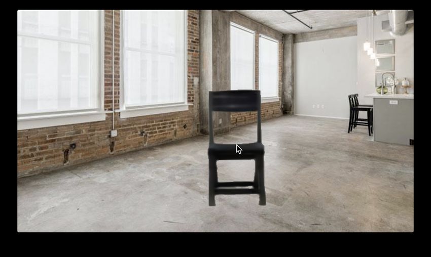
transformations thus include not only rotation and transla-                        ing a generative adversarial (GAN) training scheme [7, 27].
tion, but also effects such as non-uniform 3D scaling and                          Conditional methods then provided the ability to change the
global or local non-rigid warping. Additionally, bottleneck                        style of an input image to another style [13, 22]. Initially
representations of multiple inputs can be transformed into,                        such trained networks could only handle one style [46];
and combined in, the same coordinate frame, allowing them                          more recent works now allow multiple attribute changes us-
to be aggregated naturally in feature space. This can re-                          ing a single network, by learning to disentangle these at-
solve ambiguities present in a representation from a single                        tributes from the training images [18, 34, 47].
image. While similar to ideas in Spatial Transformer Net-                              Novel view synthesis (NVS) generates an image from a
works (STN) [15, 20] and a 3D reconstruction method [29]                           new, user specified viewpoint, given one or more images of
deriving from it, a key distinction of our approach is that the                    a scene from known viewpoints. We focus on methods that,
spatial transformations are input to our network, as opposed                       like ours, can synthesize novel views from a single input im-
to inferred by the network. It is precisely this difference that                   age. This is a highly ill-posed problem, requiring strong 3D
enables TBNs to make such diverse manipulations.                                   understanding and disentanglement of viewpoint and ob-
    We highlight the power of this approach by applying it                         ject shape from the input image. Since the seminal work
to novel view synthesis (NVS). NVS is a challenging task,                          of Hoiem et al. [12], methods have sought to develop more
requiring non-trivial 3D understanding from one or more                            expressive models to address general NVS. Early CNN so-
images in order to predict corresponding images from new                           lutions regressed output pixel color in the new view [33, 44]
viewpoints. This allows us to demonstrate both the ability                         directly from the input image. Some works disentangle their
of a TBN to naturally spatially disentangle features within                        representations [34, 44], separating pose from object [44]
a 3D bottleneck volume, and the benefits that this confers.                        or face identity [34]. Zhou et al. [45] introduced a flow pre-
We compare to leading NVS methods [33, 45, 32, 25], on                             diction formulation, inferring an output to input pixel map-
images from the ShapeNet dataset [1], and attain state-of-                         ping instead, to which an explicit occlusion detection and
the-art results on both L1 and SSIM metrics (see Table 1,                          inpainting module [25] and generalization to an arbitrary
and Figs. 1 & 3a). We present additional qualitative results                       number of input images [32] have been added. Eslami et
on a synthetic human performance dataset. We also train a                          al. [3] developed a latent representation that can be aggre-
simple voxel occupancy classifier on image segmentations                           gated to combine inputs, and show good results on synthetic
(i.e. without 3D supervision), and use it to demonstrate ac-                       geometric scenes.
curate 3D reconstructions from a single image. Finally, we                             A drawback of all these approaches is that they condi-
provide qualitative examples of how this bottleneck struc-                         tion their networks to perform the transformation, limiting
ture allows us to perform realistic, varied and creative image                     the transformations that can be applied to those that have
manipulation in 3D (Figs. 1 & 6).                                                  been learned. Most recently, methods have been proposed
    In summary, the main contributions of this work are:                           to generate explicit representations of geometry and appear-
   • A novel, transformable bottleneck framework that al-                          ance that are transformed and rendered using standard ren-
      lows CNNs to perform spatial transformations for                             dering pipelines [21, 35]. While these representations can
      highly controllable image synthesis.                                         be rendered from arbitrary viewpoints, they are based on
   • A state-of-the-art NVS system using TBNs.                                     planar representations and are therefore not able to capture
   • A method for extracting high-quality 3D structure                             realistic shape, especially when rendered from side views.
      from this bottleneck, constructed from a single image.                       Our TBN approach allows us to perform fine-grained and
   • The ability to perform realistic, varied and creative 3D                      varied, even non-rigid, 3D manipulations in the bottleneck
      image manipulation.                                                          volume, synthesizing them into realistic novel views. Here,
                                                                                   the manipulations are applied manually. However, recent
2. Related work                                                                    work [39] proposes a learned network for deforming ob-
                                                                                   jects arbitrarily (parameterized by an input shape), an idea
   We now review works related to the TBN, in the areas of                         that complements our framework.
image and novel view synthesis, and volumetric reconstruc-
tion2 and rendering.
                                                                                   2.2. Volumetric reconstruction and rendering
2.1. Image and novel view synthesis
                                                                                       Several recent methods reconstruct an explicit occu-
   Many exciting advances in image synthesis and manip-                            pancy volume from a single image [2, 5, 16, 29, 36, 42, 41,
ulation have emerged recently that enable the application                          43], some of which are trained using only supervision from
of specific styles or attributes. Early approaches generated                       2D images [29, 36, 43]. Yan et al. [43] max-pool occupancy
natural images using samples from a chosen distribution us-                        along image rays to produce segmentation masks, and min-
   2 Image to depth map [6, 19], 3D mesh [11, 14, 38], point cloud [4] and         imize their difference w.r.t. the ground-truths. Tulsiani et
surfel primitive [8] approaches also exist, but are outside the scope of our       al. [36] enforce photo-consistency between projected color
discussion.                                                                        images (given the camera poses) using the correspondences

                                                                               2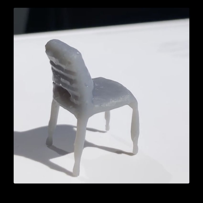
Transformable bottleneck

                       Encoder             Resampling                                             Decoder

                       2D                    Layer                     Aggregated
                                                                                                      2D
                             3D                                        Volumetric
                                                                      Representation         3D

           …                 Target pose                …       +

                       2D                                                                 Occupancy         Segmentation
                             3D                                                            Decoder            Decoder

                                                                                                                            (b) Patch-volume
                                     (a) Transformable Bottleneck Network (TBN)                                              correspondence

Figure 2: A Transformable Bottleneck Network. (a) Network architecture, consisting of three parts: an encoder (2D convolution layers,
reshaping, 3D convolution layers), a resampling layer, and a decoder (a mirror of the encoder architecture). The encoder and decoder are
connected purely via the bottleneck; no skip connections are used. The resampling layer transforms an encoded bottleneck to the target
view via trilinear interpolation. It is parameterless, i.e. transformations are applied explicitly, rather than learned. Multiple inputs can be
aggregated by averaging bottlenecks prior to decoding. (b) A visualization of the conceptual correspondence between an image patch and
a subvolume of the bottleneck. Bottleneck volume visualizations show the cellwise norm of feature vectors. It is interesting that to note
that this norm appears to encode the object shape.

implied by the occupancy volume. In contrast to these ap-                               rameterization, Fk→l , as input, and transforms the
proaches that use explicit occupancy volumes and render-                                bottleneck via a trilinear resampling operation.
ing techniques, the implicit approaches proposed by Kar et                          3. A decoder network DI : X0l → Il0 with parameters
al. [16], and in particular Rezende et al. [29], are more                               θI , whose architecture mirrors that of the encoder, that
relevant to our work—both the volumetric representation                                 decodes the transformed bottleneck, X0l , into an output
and the decoder (rendering) are learned, similar to recent                              image, Il0 .
neural rendering work [24]. The former [16], trained on                          Subscripts k and l represent viewpoints. Neither the en-
ground truth geometry to estimate geometry from images,3                         coder nor the decoder are trained to perform a transforma-
uses three learned networks4 and a hand-designed unpro-                          tion: it is fully encapsulated in the bottleneck resampling
jection step to compute a latent volume. The latter [29]                         layer. As this layer is parameterless, the network cannot
requires the target transformation to be inferred by the net-                    learn how to apply a particular transformation at all; rather,
work for NVS, whereas ours requires it to be provided as                         it is applied explicitly. A single source image synthesis op-
input, removing any limitations on the transformations that                      eration, which is end-to-end trainable, is written as:
can be applied at test time.
                                                                                              Il0 = DI (S(E(Ik , θE ), Fk→l ), θI ).           (1)
3. Transformable bottleneck networks                                             When Fk→l is the identity transform (i.e. k = l), this oper-
                                                                                 ation defines an auto-encoder network.
  In this section we formally define our Transformable
Bottleneck Network architecture and training method.                             3.1.1. Handling multiple input views
                                                                                     Our formulation naturally extends to an arbitrary num-
3.1. Architecture                                                                ber of inputs, both for training and testing, without mod-
A TBN architecture (Fig. 2(a)) consists of three blocks:                         ifications to either encoder or decoder. The encoded and
 1. An encoder network E : Ik → Xk with parame-                                  transformed representations of all inputs are simply aver-
    ters θE , that takes in an image Ik and, through a se-                       aged:
    ries of 2D convolutions, reshaping, and 3D convolu-                                                  1 X
    tions,5 outputs a bottleneck representation, Xk , struc-                                     X0l =          S(Xk , Fk→l ),           (2)
                                                                                                        |K|
    tured as a volumetric grid of cells, each containing an                                                     k∈K
    n-dimensional feature vector.                                                where K is the set of input viewpoints. The number of in-
 2. A parameterless bottleneck resampling layer                                  puts tested on can differ from the number trained on, which
    S : Xk , Fk→l → X0l , that takes a bottleneck rep-                           can differ even within a training batch. We later show that
    resentation and user-provided transformation pa-                             the model trained with a single input view can effectively
   3 The latent representation therefore does not encode appearance.
                                                                                 aggregate multiple inputs at inference time, and also that a
   4 For 2D image encoding, recurrent fusion and a 3D grid reasoning.            model trained on multiple inputs can perform state-of-the-
   5 See the appendix for the exact architecture.                                art inference from a single image.

                                                                             3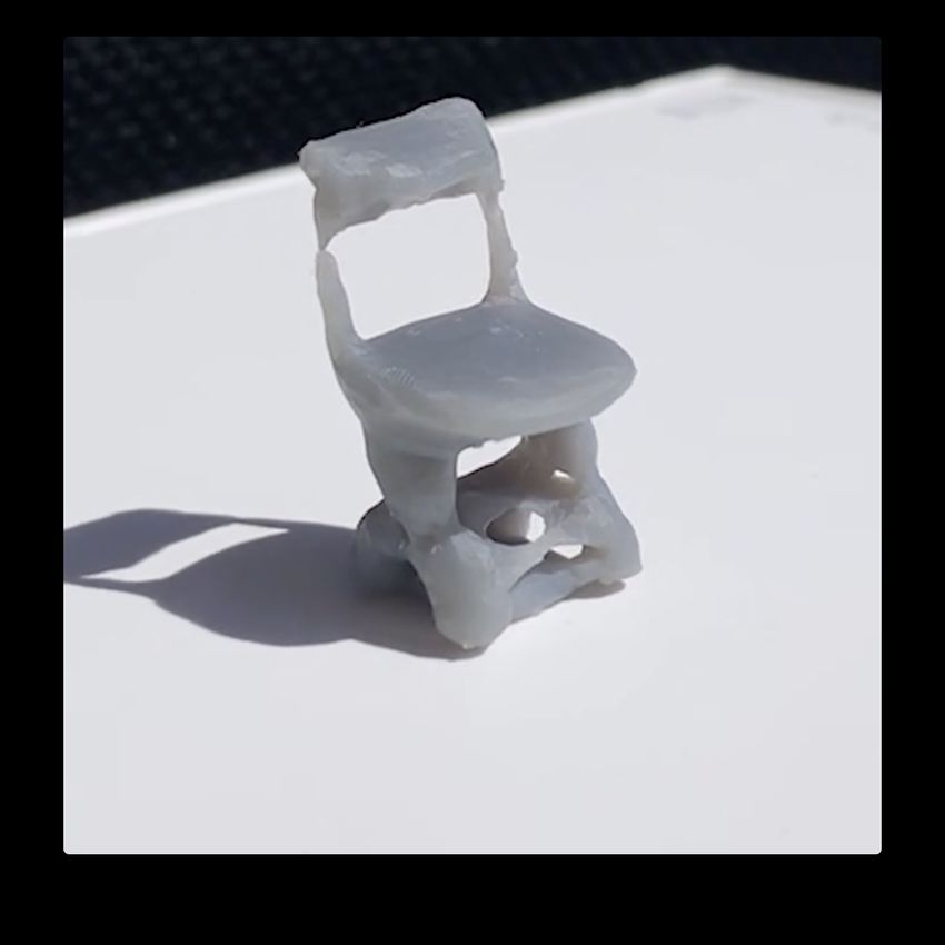
3.1.2. Bottleneck layout and resampling                                         3.2.1. Appearance supervision
    The network architecture defines the number of cells                           NVS requires a minimum of two images of a given ob-
along each side of the bottleneck volume, but not the spa-                      ject from different, known viewpoints.8 Given {Ik , Il } and
tial position of each cell. Indeed, the framework imposes                       Fk→l , we can compute a reconstruction, Il0 , of Il using
no constraints on their position, e.g. the voxel grid cells do                  equation (1). Using this, we define several losses in image
not need to be equally spaced. In this work the grid cells                      space with which to train our network parameters. The first
are chosen to be equally spaced,6 with the volume centered                      two are a pixel-wise L1 reconstruction loss and an L2 loss in
on the target object and axis aligned with the camera co-                       the feature space of the VGG-19 network, often termed as
ordinate frame. Perspective effects caused by projection                        the perception loss:
through a pinhole camera, and the camera parameters that
affect them (such as focal length), are learned in the encoder                            LR (θE , θI ) = ||Ik→l − Il ||1 ,                             (4)
and decoder networks, rather than handled explicitly.
                                                                                                          X
                                                                                          LP (θE , θI ) =     ||Vi (Ik→l ) − Vi (Il )||22 ,             (5)
    Since the bottleneck representation is a volume, it can be                                                 i
resampled via trilinear interpolation, which is fully differ-
entiable [15, Eqn. 9]. This allows it to be spatially trans-                    where Vi is the output of the ith layer of the VGG-19 net-
formed. The transformation, Fk→l , is parameterized as a                        work. To enforce structural similarity of the outputs we
flow field that, for each output grid cell, defines the 3D point                also adopt the structural similarity loss [31, 40], denoted as
in the input volume to sample to generate it. The decoder                       LS . Finally, we employ the adversarial loss of Tulyakov et
takes as input a volume of the same dimensions as the en-                       al. [37], LA , to increase the sharpness of the output image.
coder produces, therefore the flow field also has these di-
                                                                                3.2.2. Segmentation supervision
mensions. Feature channels form separate volumes that are
resampled independently, then recombined to form the out-                           Appearance supervision is sufficient for NVS tasks, but
put volume.                                                                     to compute a 3D reconstruction we also require segmenta-
    When the view transformation is rigid, as in the case of                    tion supervision,9 in order to learn θO and θS . We therefore
NVS, the flow field is computed by transforming the cell                        assume that for each image Ii we also have a binary mask
coordinates of the novel view by the inverse of the relative                    Mi , with ones on the foreground object pixels and zeros
transformation from the input view.7 Non-rigid deforma-                         elsewhere.10 Segmentation losses are computed in all input
tions can also be applied, enabling creative shape manip-                       and output views, using the aggregated bottleneck in the
ulation, which we demonstrate in Sec. 4.4. Importantly, we                      multi-input case, as follows:
do not train on these kinds of transformations.                                                         X
                                                                                   LM (θE , θO , θS ) =     H(DS (S(Ol , Fl→k ), θS ), Mk ),
3.1.3. Geometry decoder                                                                                    k∈K
    Since the TBN spatially disentangles shape and appear-                                                   + H(DS (Ol , θS ), Ml ),                   (6)
ance within the volumetric bottleneck, it should also be able
to reconstruct an object in 3D from the bottleneck represen-                    where Ol = DO (X0l , θO ) and H is the binary cross en-
tation. Indeed, prior work [29, 36] shows that training a                       tropy cost, summed over all pixels. Summing over all views
3D reconstruction using the NVS task alone, i.e. without                        achieves a kind of space carving. Correctly reconstructing
3D supervision, is possible. We extract shape in the form                       unoccupied cells within the visual hull is difficult to learn
of a scalar occupancy volume, O, with one value per bot-                        as no 3D supervision is used, but appearance supervision
tleneck cell, using a separate, shallow network, occupancy                      helps address this.
decoder, DO : X → O. To avoid using any 3D supervision
                                                                                3.2.3. Optimization
to train this decoder, we then apply another decoding layer,
DS : O → S, that applies a 1D convolution along the z-                             The total training loss, with hyper-parameters λi to con-
axis (the optical axis), followed by a sigmoid, to generate a                   trol the contribution of each component, is
scalar segmentation image S, thus:
                                                                                   LT (Θ) = LR + λ1 LP + λ2 LS + λ3 LA + λ4 LM ,                        (7)
             S = DS (O, θS ),        O = DO (X, θO ),                (3)
                                                                                This loss is fully differentiable, and the network can be
where θO and θS are the parameters of the occupancy and
                                                                                trained end-to-end by minimizing the loss w.r.t. the network
segmentation decoders respectively.
                                                                                parameters Θ = {θE , θI , θO , θS } using gradient descent.
3.2. Training                                                                       8 Viewpoints are defined by camera rotation and translation, w.r.t. some

   We train the TBN using the NVS task as follows.                              arbitrary reference frame; world coordinates are not required.
                                                                                    9 3D supervision could be used, but requires ground truth 3D data.
   6 The scale of the spacing is unimportant here, as our NVS experiments          10 Segmentation supervision is not a hard constraint, therefore segmen-
only involve camera rotations around the object center.                         tations from state-of-the-art methods (e.g. Mask R-CNN [9]) may suffice.
   7 The flow is defined from output voxel to input voxel coordinate.           However, we use ground truth masks in this work.

                                                                            4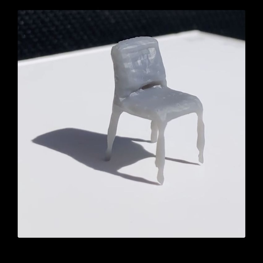
1 input   2 inputs   3 inputs   4 inputs
                                                                                                                                                               Target

                                                                                                  Sun et al.
                                                                                                                                                            Input views

                                                                                                  Ours
                                                                                                                                                              Target

                                                                                                  Sun et al.
                                                                                                                                                            Input views

                                                                                                  Ours
                             (a) Results on novel view synthesis                                               (b) Comparisons with Sun et al. [32]
Figure 3: Qualitative results and comparisons. (a) Randomly selected NVS samples generated using our method. Left: input images
(3 of the 4 used). Middle: transformable bottleneck and 3D reconstruction. Right: synthesized output views. (b) Samples of synthesized
novel views using the method of Sun et al. [32] and ours. Their method fails to capture overall structure for chairs, and generates unnatural
artifacts on cars, especially around the wheels. Where < 4 input views are used, they are selected in clockwise order, starting top left.

4. Experiments                                                           from a variety of object categories. We measure the capa-
                                                                         bility of our approach to synthesize new views of objects
   We train and evaluate our framework on a variety of                   under large transformations, for which ground-truth results
tasks. We provide quantitative evaluations for our results               are available. We train and evaluate our approach using the
for novel view synthesis using both single and multi-view                cars and chairs categories, to demonstrate its performance
input, and compare our results to state-of-the-art methods               on objects with different structural properties. Each model
on an established benchmark. We also perform 3D object                   is rendered as 256 × 256 RGB images at 18 azimuth an-
reconstruction from a single image and quantitatively com-               gles sampled at 20-degree intervals and 3 elevations (0, 10
pare our results to recent work [36]. Finally, we provide                and 20 degrees), for a total of 54 views per model. We
qualitative examples of our approach applying creative ma-               use standard training and test data splits [25, 32, 45], and
nipulations via non-rigid deformations.                                  train a separate network for each object category (also stan-
4.1. A note on implementation                                            dard), using 4 input images to synthesize the target view.
                                                                         The network architecture and training method were fixed
    Our models are implemented and trained using the Py-                 across categories.
Torch framework [26], for automatic differentiation and                      As described in Section 3.1.1, our framework can use
parallelized computation for training and inference. We ex-              a variable number of input images. Though trained with
tended this framework to include a layer to perform par-                 4 input images, we demonstrate that our networks can in-
allelizable trilinear resampling of a tensor, in order to ef-            fer high-quality target images using fewer input images
ficiently perform our spatial transformations. We plan to                at test time. Using the experimental protocol of Sun et
release the source code for our framework to the research                al. 2018 [32], which uses up to 4 input images to infer a
community upon publication.                                              target image, we report quantitative results for our approach
    Each network was trained on 4 NVIDIA P100s, with                     and others that can use multiple input images [32, 33, 45],
each batch distributed across the GPUs. As we found that                 as well as for an approach accepting single inputs [25].
batch size had no discernible effect on the final result, we                 To further demonstrate the applicability of our method
selected it to maximize GPU utilization. We trained each                 to non-rigid objects with higher pose diversity and lower
model until convergence on the test image set, which took                appearance diversity, we also train and qualitatively evalu-
approximately 8 days. For more details on the network ar-                ate a network using a multi-view human action dataset [28].
chitecture, training process and datasets used in our evalua-            This dataset uses a limited number (186) of textured CAD
tions and results, please consult the appendix.                          models representing human subjects. However, the subjects
4.2. Novel view synthesis                                                are rigged to perform animation sequences representing a
                                                                         variety of common activities (running, waving, jumping,
  Setup. We use renderings of objects obtained from the                  etc.), resulting in a much larger number of renderings. Note
ShapeNet [1] dataset, which provides textured CAD models

                                                                     5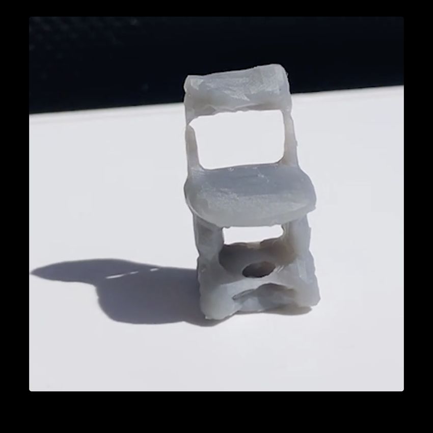
Methods                      Car           Chair         dence between local regions of source and target images
                                                L1       SSIM   L1      SSIM       cause artifacts, such as the wheel on the front of the car in
                 Tatarchenko et al. 2015 [33]   .139     .875   .223    .882       row 5. In contrast, our method recovers the overall struc-
                    Zhou et al. 2016 [45]       .148     .877   .229    .871       ture of both chairs and cars well, improving finer details
       1 view

                     Park et al. 2017 [25]      .119     .913   .202    .889
                     Sun et al. 2018 [32]       .098     .923   .181    .895       as additional input views are added. We note that their re-
                             Ours               .091     .927   .178    .895       sults are generally sharper, as they use flow prediction to di-
                 Tatarchenko et al. 2015 [33]   .124     .883   .209    .890       rectly sample input pixels to construct the output, whereas
       2 views

                    Zhou et al. 2016 [45]       .107     .901   .207    .881       our output images are rendered entirely from the bottleneck
                     Sun et al. 2018 [32]       .078     .935   .141    .911
                            Ours                .072     .939   .136    .928       representation, as is required for general 3D manipulation.
                 Tatarchenko et al. 2015 [33]   .116     .887   .197    .898
                                                                                   4.3. Appearance synthesis for 3D reconstruction
       3 views

                    Zhou et al. 2016 [45]       .089     .915   .188    .887
                     Sun et al. 2018 [32]       .068     .941   .122    .919
                            Ours                .063     .943   .116    .936
                                                                                       As reported above, our method performs well on NVS
                                                                                   with a single view, and progressively improves as more in-
                 Tatarchenko et al. 2015 [33]   .112     .890   .192    .900
                                                                                   put views are used. We now show that this trend extends to
       4 views

                    Zhou et al. 2016 [45]       .081     .924   .165    .891
                     Sun et al. 2018 [32]       .062     .946   .111    .925       3D reconstruction. However, given that more views aid re-
                            Ours                .059     .946   .107    .939
                                                                                   construction, and that our network can generate more views,
Table 1: Quantitative results on novel view synthesis. We report                   an interesting question is whether the generative power of
the L1 loss (lower is better) and the structural similarity (SSIM) in-             our network can be used to aid the 3D reconstruction task.
dex (higher is better) for our method and several baseline methods,                We ran experiments to find out.
for 1 to 4 input views, on both car and chair ShapeNet categories.                     Setup. To evaluate our method, we use the 3D recon-
                                                                                   struction evaluation framework from the Differentiable Ray
that the training process is identical to that used for rigid                      Consistency (DRC) work of Tulsiani et al. [36], which in-
objects—input images for a given scene see the subject in a                        fers a 3D occupancy volume from a single RGB image. We
fixed pose. Thus, the capability to perform non-rigid trans-                       trained our network on their dataset: multi-view images of
formations, as seen in Sec. 4.4, is still implicitly learned by                    ShapeNet objects, rendered under varying lighting condi-
the network.                                                                       tions from 10 viewpoints, randomly sampled from uniform
    Results. Table 1 reports quantitative results across recent                    azimuth and elevation distributions with ranges [0, 360) and
methods, for 1 to 4 input views, on car and chair categories,                      [−20, 30], respectively. As our method is trained using a
for both the L1 cost (averaged across all foreground pixels in                     set of multi-view images and corresponding segmentation
all target views, as in [45]) and structural similarity (SSIM)                     masks, we compare our method to their publicly available
scores [40]. Though our networks are trained using exactly                         model trained on masked, color images, using 5 random
4 input views, we obtain state-of-the-art results across all                       views of each object. In contrast, for this task our model
metrics, categories and number of input views, even in the                         was trained using only 2 random views (one input, one out-
challenging case of single-view input.                                             put) of each object.
    These results indicate that the TBN excels at NVS, and                             Using the DRC [36] experimental protocol, we report
outperforms alternatives using both pixelwise and percep-                          the mean intersection-over-union (IoU) of the volumes from
tual metrics. We further note that our method performs sig-                        our occupancy decoder, computed on the evaluation im-
nificantly better than others in cases involving large trans-                      age set, compared to the ground-truth occupancies obtained
formations of the input images and challenging viewpoints                          by voxelizing the 3D meshes used to render these images.
(see Fig. 3b). This demonstrates that our approach to com-                         Like DRC, we report the IoU attained using the optimal dis-
bining information from these viewpoints is an effective                           cretization threshold for each object category.
strategy for synthesizing novel viewpoints, in addition to                             Results. Figure 4 shows the results of this evaluation.
having other interesting applications (see below).                                 We report IoU numbers obtained using one real input im-
    Fig. 3a shows qualitative examples on 3 datasets: the                          age, with 0 to 9 additional synthesized views, sampled ei-
ShapeNet cars and chairs used for our quantitative eval-                           ther randomly (red line) or regularly (at 0◦ elevation, blue
uations, and the aforementioned human activity dataset.                            line). For comparison, we show results using additional real
Fig. 3b qualitatively compares our results with those of Sun                       images of the target object (green line), randomly sampled
et al. [32] on several challenging examples requiring large                        from the evaluation set (regularly sampled images were not
viewpoint transformations from the chair and car datasets.                         available), as well as the results using DRC [36] with a sin-
Their method has difficulty inferring the proper correspon-                        gle input image (yellow line). The figure also contains qual-
dence between the source and target images for both ob-                            itative comparisons of results11 using our best method (reg-
ject categories, particularly the more complex and variable                        ularly sampled synthetic images) with varying numbers of
structure of the chairs. Thus, many details are missing or                         synthetic images (middle columns), compared to DRC [36]
incorrectly transformed. For cars, errors in the correspon-                          11 We   render the voxel grids as meshes using an isosurface method.

                                                                               6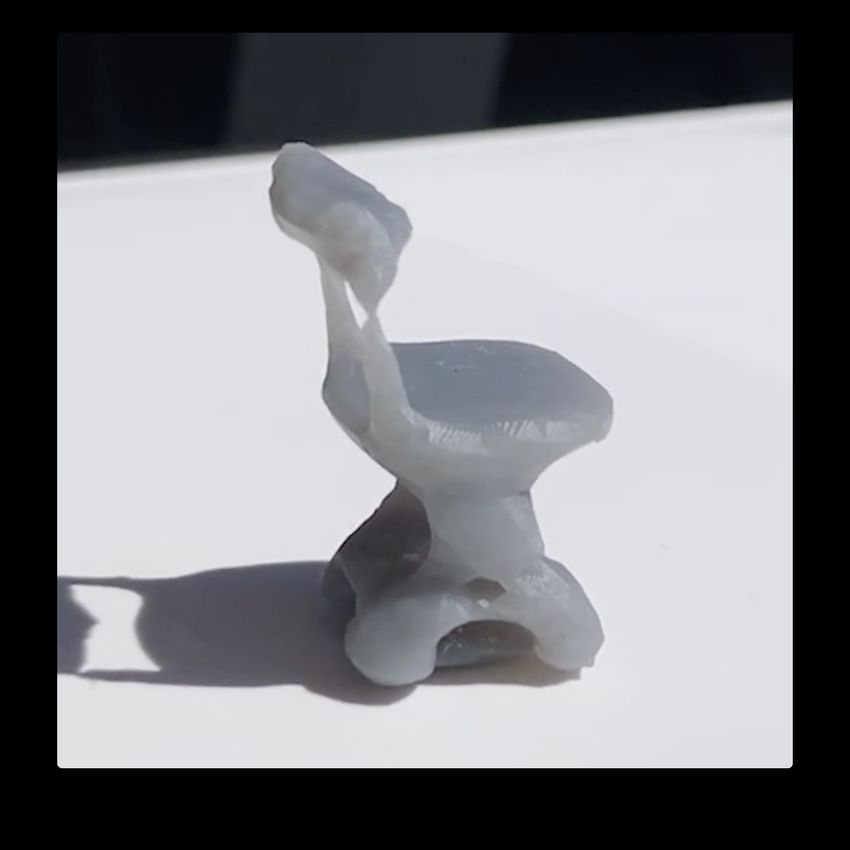
DRC           TBN using synthesized views                           GT               Input images   Output mesh   Views of 3D printed reconstruction

                                                                                                                     Figure 5: Examples of 3D printed objects created using our ap-
                                                                                                                     proach to 3D reconstruction.

                             0.50                                                                                    so as to produce a plausible image under this transforma-
                                                                                                                     tion. Therefore, consider a chair viewed from only one an-
    3D reconstruction, IoU

                             0.44
                                                                                                                     gle: the encoder could say where in space it believes the
                             0.38
                                                                                                                     visible parts be, allowing it to be transformed, then the de-
                                                      TBN, synthesized views, regular pose sampling
                                                                                                                     coder could see this partial reconstruction in the bottleneck,
                             0.31                     TBN, real views, random pose sampling                          and knowing what chairs look like, hallucinate the unseen
                                                      DRC (1 view), Tulsiani et al. 2017
                                                      Synthesized
                                                      TBN, synthesizedviews,     random
                                                                        views, random   posepose  sampling
                                                                                            sampling                 parts. By recycling the synthesized image back through the
                             0.25
                                    0     1   2      3       4       5      6             7        8         9       encoder, it could then see new parts of the chair, and gen-
                                                  # extra synthesized views
                                                                                                                     erate structure for them also. In essence, it comes down to
Figure 4: 3D reconstruction results. Quantitative (IoU, follow-                                                      where unseen structure is hallucinated within the network.
ing the evaluation framework of Tulsiani et al. [36]) and qualitative                                                Since the bandwidths of our encoder and image decoder
results of our method performing 3D reconstruction on the chairs                                                     are identical, there is no reason for it be in any particular
dataset, from a single input image, supplemented by additional                                                       part. However, because the gradients in the decoder lay-
views synthesized by our network. 0 synthesized views indicates                                                      ers have been passed through fewer other layers, they may
that only the original input image is used, while 1 to 9 indicate                                                    receive a stronger signal for hallucination from the output
that we synthesize these additional views and combine the bottle-
                                                                                                                     view, hence learn it first.
necks generated from these viewpoints with those obtained from
the original input view. Results from Tulsiani et al. [36], who use                                                      One might expect the occupancy decoder to learn to hal-
only one image during inference, are also shown.                                                                     lucinate structure as well as the image decoder, but our re-
                                                                                                                     sults indicate that it doesn’t (see our qualitative reconstruc-
                                                                                                                     tions with no synthetic views, in Fig. 4). We intuit that this
(left) and the ground truth (right). Our method produces                                                             is because it has much less information (binary vs. color im-
good results even with concavities (Fig. 4, row 1), that could                                                       ages) to train on, and concomitantly a significantly smaller
not be obtained solely from the object’s silhouette, demon-                                                          bandwidth. This further validates our hypothesis that ap-
strating that NVS supervision is an able substitute for ge-                                                          pearance supervision improves 3D reconstruction within
ometry supervision when inferring the geometric structure                                                            the visual hull, in the absence of 3D supervision.
of such objects.                                                                                                         Physical recreations of real objects. An exciting possi-
    Using synthesized views from random poses clearly im-                                                            bility of image-based reconstruction is being able to recre-
proves the reconstruction quality as more views are incor-                                                           ate old objects from photographs. We took 3 photos each
porated into our representation, though does not match the                                                           of 2 real chairs, computed TBNs from these images and
quality attained when using the same number of real images                                                           aggregated them using estimated relative poses. We com-
instead. Using synthetic views sampled at regular intervals                                                          puted occupancy volumes from these, extracted meshes us-
around the object’s central axis produces significantly bet-                                                         ing an isosurface method, and 3D printed these meshes.
ter results, achieving superior single view 3D reconstruc-                                                           Figure 5 shows the input images, reconstructed meshes and
tion to all other methods when using as few as 3 synthetic                                                           3D printed objects. Despite the low resolution of the occu-
views. This dramatic improvement from randomly to regu-                                                              pancy volume (403 voxels), these physical recreations are
larly sampled synthetic views can be explained by the fact                                                           coherent and depict the salient details of each chair.
that information from each of the regularly sampled views
is much more complementary than for the random views,
that could leave parts of the object “unseen” (or unhalluci-                                                         4.4. Non-rigid transformations
nated). That synthetic views should improve the results at                                                              Spatial disentanglement. Due to the convolutional na-
all is a more nuanced argument.                                                                                      ture of our network, a subvolume of the 3D bottleneck
    One might imagine that recycling hallucinated views into                                                         broadly corresponds to a patch of the input (if encoding)
the encoder would simply reinforce the existing reconstruc-                                                          or output (if decoding) image, as visualized in Fig. 2(b).
tion. However, we argue the following: the encoder learns                                                            Any of the features in the subvolume, or a combination of
to extract the features that allow an image to be transformed,                                                       them, can account for the appearance of the image patch;
and the decoder learns to process the transformed features                                                           there is no guarantee that the features used will come from

                                                                                                                 7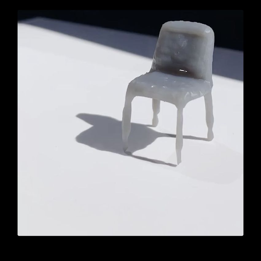
stretching stretching Input images Novel views Manipulated shapes
Horizontal Vertical
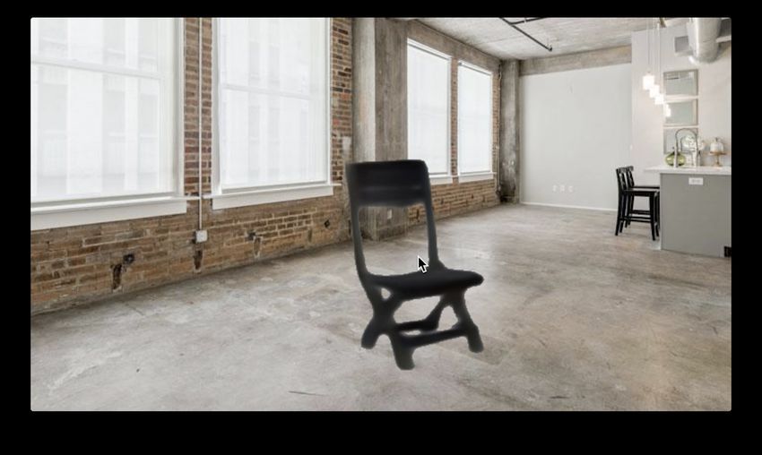
Figure 7: Interactive manipulation. We use our approach to ro-
tate and deform objects before compositing them into real images.
Inflation Slicing & stitching Twisting
Interactive creative manipulation. We implemented a
tool to demonstrate a useful real-world application of the
TBN: interactive manipulation and compositing. The user
has one or more13 photos of an object (whose class has been
trained on) they wish to manipulate and place in a photo of
a real world scene. The images are loaded into our appli-
cation, from which a single aggregated bottleneck is com-
puted. An interactive interface then allows the user to rotate,
translate, scale and stretch the object, transforming and ren-
dering the bottleneck in realtime and overlaying the object
Figure 6: Creative, non-rigid manipulations (view as videos in in the target image, as they apply the transformations.
Acrobat Reader). Selected examples of non-rigid 3D manipula-
Figure 7 contains example inputs and outputs of this pro-
tions applied to transformable bottlenecks, for creative image and
video12 synthesis. Manipulations include: vertical and horizontal cess, for an interior design visualization use case. Two pho-
stretching, twisting, slicing & stitching, non-linear inflation. tos of a real chair were provided (with estimated relative
pose). Rotations and stretches were then applied interac-
tively, to get a feel for how the chair would look with dif-
the voxels corresponding to the location in 3D space of the ferent orientations and styles. Despite the challenging na-
surface seen in the patch. In our framework, however, 2D ture of this example (real photos of a chair with complex
supervision from multiple directions (both input and output structure, and real-world lighting conditions such as specu-
views) places multiple subvolume constraints on where in- lar highlights), we achieve highly plausible results.
formation can be stored. Storing information in the cells
corresponding to the location in 3D space of the visible sur-
5. Conclusion
face is the most efficient layout of information that meets all
of those constraints, thus the one which achieves the lowest This work has presented a novel approach to applying
loss given the available network bandwidth. The effect is spatial transformations in CNNs: applying them directly
therefore achieved implicitly, rather than explicitly. to a volumetric bottleneck, within an encoder-bottleneck-
Creative manipulation. Based on this effect of spatial decoder network that we call the Transformable Bottleneck
disentanglement, arbitrary non-rigid volumetric deforma- Network. Our results indicate that TBNs are a powerful
tions can be applied on the transformable bottleneck, re- and versatile method for learning and representing the 3D
sulting in a similar transformation of shape of the rendered structure within an image. Using this representation, one
object. We demonstrate this qualitatively with a variety cre- can intuitively perform meaningful spatial transformations
ative tasks, shown in Figure 6, that are performed by manip- to the extracted bottleneck, enabling a variety of tasks.
ulating and combining the volumetric bottlenecks extracted We demonstrate state-of-the-art results on NVS of ob-
from input images. By rotating the upper and lower por- jects, producing high quality reconstructions by simply ap-
tion of the volume in opposite directions (top row), we can plying a rigid transformation to the bottleneck correspond-
transform different regions of the target into a new shape ing to the desired view. We also demonstrate that the 3D
that does not correspond to a single rigid transformation. structure learned by the network when trained on the NVS
Non-uniform and/or local scaling can be applied to inflate task can be straightfowardly extracted from the bottleneck,
(second row) or stretch and shrink (third row) objects. Parts even without 3D supervision, and furthermore, that the
of a bottleneck can even be replaced with another part from powerful generative capabilities of the complete encoder-
the same, or a different bottleneck, creating hybrid objects decoder network can be used to substantially improve the
(bottom row). Many other such manipulations are possible, quality of the 3D reconstructions by re-encoding regularly
far beyond the scope of the rigid transformations trained on. spaced, synthetic novel views. Finally, and perhaps most in-
triguingly, we demonstrate that a network trained on purely
12 While such manipulations could seem simple to achieve in 2D (we rigid transformations can be used to apply arbitrary, non-
disagree), an edited 3D object can also be rendered consistently from any rigid, 3D spatial transformations to content in images.
azimuth (see videos here and in the supplementary video), from a single
manipulated bottleneck. 13 Multiple images require true or estimated relative poses.
8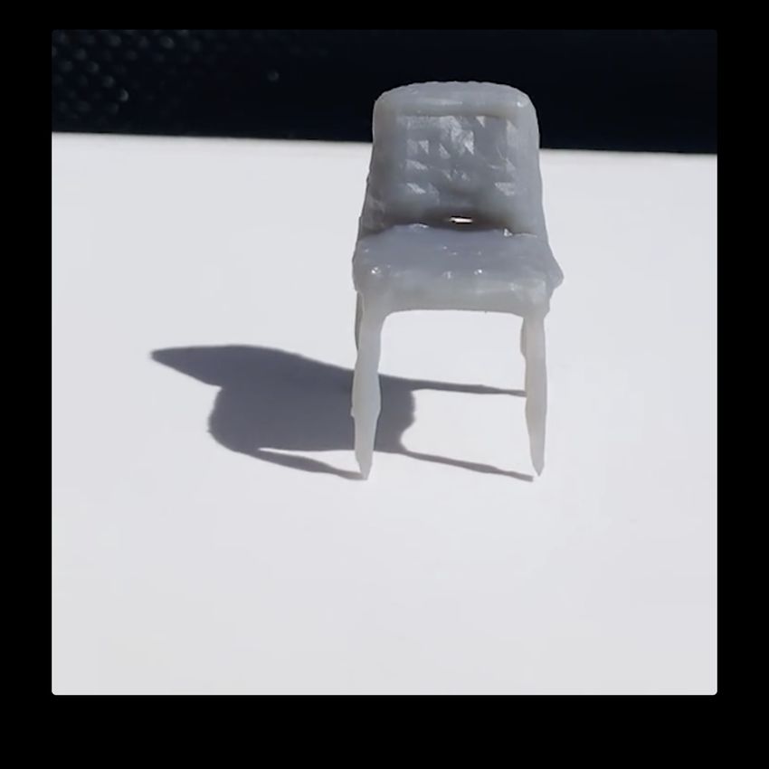
References                                                               [17] D. P. Kingma and J. Ba. Adam: A method for stochastic
                                                                              optimization. CoRR, abs/1412.6980, 2014.
 [1] A. X. Chang, T. Funkhouser, L. Guibas, P. Hanrahan,                 [18] G. Lample, N. Zeghidour, N. Usunier, A. Bordes, L. De-
     Q. Huang, Z. Li, S. Savarese, M. Savva, S. Song, H. Su,                  noyer, et al. Fader networks: Manipulating images by sliding
     et al. Shapenet: An information-rich 3d model repository.                attributes. In Proceedings of the Neural Information Process-
     arXiv preprint arXiv:1512.03012, 2015.                                   ing Systems Conference, pages 5967–5976, 2017.
 [2] C. B. Choy, D. Xu, J. Gwak, K. Chen, and S. Savarese. 3d-
                                                                         [19] Z. Li and N. Snavely. Megadepth: Learning single-view
     r2n2: A unified approach for single and multi-view 3d object
                                                                              depth prediction from internet photos. In Proceedings of the
     reconstruction. In Proceedings of the European Conference
                                                                              IEEE Conference on Computer Vision and Pattern Recogni-
     on Computer Vision, 2016.
                                                                              tion, pages 2041–2050, 2018.
 [3] S. A. Eslami, D. J. Rezende, F. Besse, F. Viola, A. S. Mor-
                                                                         [20] C.-H. Lin and S. Lucey. Inverse compositional spatial trans-
     cos, M. Garnelo, A. Ruderman, A. A. Rusu, I. Danihelka,
                                                                              former networks. In Proceedings of the IEEE Conference on
     K. Gregor, et al. Neural scene representation and rendering.
                                                                              Computer Vision and Pattern Recognition, 2017.
     Science, 360(6394):1204–1210, 2018.
 [4] H. Fan, H. Su, and L. J. Guibas. A point set generation             [21] M. Liu, X. He, and M. Salzmann. Geometry-aware deep
     network for 3d object reconstruction from a single image.                network for single-image novel view synthesis. In Proceed-
     In Proceedings of the IEEE Conference on Computer Vision                 ings of the IEEE Conference on Computer Vision and Pattern
     and Pattern Recognition, pages 605–613, 2017.                            Recognition, 2018.
 [5] R. Girdhar, D. F. Fouhey, M. Rodriguez, and A. Gupta.               [22] M.-Y. Liu, T. Breuel, and J. Kautz. Unsupervised image-to-
     Learning a predictable and generative vector representation              image translation networks. In Proceedings of the Neural In-
     for objects. In Proceedings of the European Conference on                formation Processing Systems Conference, pages 700–708,
     Computer Vision, 2016.                                                   2017.
 [6] C. Godard, O. Mac Aodha, and G. J. Brostow. Unsuper-                [23] L. Ma, X. Jia, Q. Sun, B. Schiele, T. Tuytelaars, and
     vised monocular depth estimation with left-right consistency.            L. Van Gool. Pose guided person image generation. In Pro-
     In Proceedings of the IEEE Conference on Computer Vision                 ceedings of the Neural Information Processing Systems Con-
     and Pattern Recognition, pages 270–279, 2017.                            ference, pages 405–415, 2017.
 [7] I. Goodfellow, J. Pouget-Abadie, M. Mirza, B. Xu,                   [24] T. Nguyen-Phuoc, C. Li, S. Balaban, and Y. Yang. Render-
     D. Warde-Farley, S. Ozair, A. Courville, and Y. Bengio. Gen-             net: A deep convolutional network for differentiable render-
     erative adversarial nets. In Proceedings of the Neural Infor-            ing from 3d shapes. In Proceedings of the Neural Informa-
     mation Processing Systems Conference, pages 2672–2680,                   tion Processing Systems Conference, 2018.
     2014.                                                               [25] E. Park, J. Yang, E. Yumer, D. Ceylan, and A. C.
 [8] T. Groueix, M. Fisher, V. G. Kim, B. Russell, and M. Aubry.              Berg. Transformation-grounded image generation network
     AtlasNet: A Papier-Mâché Approach to Learning 3D Sur-                  for novel 3d view synthesis. In Proceedings of the IEEE Con-
     face Generation. In Proceedings of the IEEE Conference on                ference on Computer Vision and Pattern Recognition, 2017.
     Computer Vision and Pattern Recognition, 2018.                      [26] A. Paszke, S. Gross, S. Chintala, G. Chanan, E. Yang, Z. De-
 [9] K. He, G. Gkioxari, P. Dollár, and R. Girshick. Mask r-                 Vito, Z. Lin, A. Desmaison, L. Antiga, and A. Lerer. Auto-
     cnn. In Proceedings of the IEEE International Conference                 matic differentiation in pytorch. 2017.
     on Computer Vision, 2017.                                           [27] A. Radford, L. Metz, and S. Chintala. Unsupervised repre-
[10] K. He, X. Zhang, S. Ren, and J. Sun. Deep residual learning              sentation learning with deep convolutional generative adver-
     for image recognition. CoRR, abs/1512.03385, 2015.                       sarial networks. 2015.
[11] P. Henderson and V. Ferrari. Learning to generate and recon-
                                                                         [28] Renderpeople, 2018. http://renderpeople.com.
     struct 3d meshes with only 2d supervision. In Proceedings
                                                                         [29] D. J. Rezende, S. A. Eslami, S. Mohamed, P. Battaglia,
     of the British Machine Vision Conference, 2018.
                                                                              M. Jaderberg, and N. Heess. Unsupervised learning of 3d
[12] D. Hoiem, A. A. Efros, and M. Hebert. Automatic photo
                                                                              structure from images. In Proceedings of the Neural Infor-
     pop-up. In ACM Transactions on Graphics, volume 24,
                                                                              mation Processing Systems Conference, 2016.
     pages 577–584. ACM, 2005.
[13] P. Isola, J.-Y. Zhu, T. Zhou, and A. A. Efros. Image-to-image       [30] O. Ronneberger, P. Fischer, and T. Brox. U-net: Convolu-
     translation with conditional adversarial networks. In Pro-               tional networks for biomedical image segmentation. CoRR,
     ceedings of the IEEE Conference on Computer Vision and                   abs/1505.04597, 2015.
     Pattern Recognition, 2017.                                          [31] J. Snell, K. Ridgeway, R. Liao, B. D. Roads, M. C. Mozer,
[14] D. Jack, J. K. Pontes, S. Sridharan, C. Fookes, S. Sareh,                and R. S. Zemel. Learning to generate images with percep-
     F. Maire, and A. Eriksson. Learning free-form deformations               tual similarity metrics. In Proceedings of the IEEE Interna-
     for 3d object reconstruction. Proceedings of the Asian Con-              tional Conference on Image Processing, 2017.
     ference on Computer Vision, 2018.                                   [32] S.-H. Sun, M. Huh, Y.-H. Liao, N. Zhang, and J. J. Lim.
[15] M. Jaderberg, K. Simonyan, A. Zisserman, et al. Spatial                  Multi-view to novel view: Synthesizing novel views with
     transformer networks. In Proceedings of the Neural Infor-                self-learned confidence. In Proceedings of the European
     mation Processing Systems Conference, 2015.                              Conference on Computer Vision, 2018.
[16] A. Kar, C. Häne, and J. Malik. Learning a multi-view stereo        [33] M. Tatarchenko, A. Dosovitskiy, and T. Brox. Single-view
     machine. In Proceedings of the Neural Information Process-               to multi-view: Reconstructing unseen views with a convolu-
     ing Systems Conference, pages 365–376, 2017.                             tional network. CoRR abs/1511.06702, 1(2):2, 2015.

                                                                     9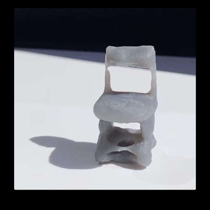
[34] L. Tran, X. Yin, and X. Liu. Disentangled representation
     learning gan for pose-invariant face recognition. In Proceed-
     ings of the IEEE Conference on Computer Vision and Pattern
     Recognition, 2017.
[35] S. Tulsiani, R. Tucker, and N. Snavely. Layer-structured 3d
     scene inference via view synthesis. In Proceedings of the
     European Conference on Computer Vision, 2018.
[36] S. Tulsiani, T. Zhou, A. A. Efros, and J. Malik. Multi-view
     supervision for single-view reconstruction via differentiable
     ray consistency. In Proceedings of the IEEE Conference on
     Computer Vision and Pattern Recognition, 2017.
[37] S. Tulyakov, M.-Y. Liu, X. Yang, and J. Kautz. Mocogan:
     Decomposing motion and content for video generation. In
     Proceedings of the IEEE Conference on Computer Vision
     and Pattern Recognition, 2018.
[38] N. Wang, Y. Zhang, Z. Li, Y. Fu, W. Liu, and Y.-G. Jiang.
     Pixel2mesh: Generating 3d mesh models from single rgb im-
     ages. In Proceedings of the European Conference on Com-
     puter Vision, pages 52–67, 2018.
[39] W. Wang, D. Ceylan, R. Mech, and U. Neumann. 3dn: 3d de-
     formation network. In Proceedings of the IEEE Conference
     on Computer Vision and Pattern Recognition, 2019.
[40] Z. Wang, A. C. Bovik, H. R. Sheikh, and E. P. Simoncelli.
     Image quality assessment: from error visibility to struc-
     tural similarity. IEEE Transactions on Image Processing,
     13(4):600–612, 2004.
[41] J. Wu, Y. Wang, T. Xue, X. Sun, B. Freeman, and J. Tenen-
     baum. Marrnet: 3d shape reconstruction via 2.5d sketches.
     In Proceedings of the Neural Information Processing Sys-
     tems Conference, 2017.
[42] J. Wu, C. Zhang, T. Xue, B. Freeman, and J. Tenenbaum.
     Learning a probabilistic latent space of object shapes via 3d
     generative-adversarial modeling. In Proceedings of the Neu-
     ral Information Processing Systems Conference, 2016.
[43] X. Yan, J. Yang, E. Yumer, Y. Guo, and H. Lee. Perspective
     transformer nets: Learning single-view 3d object reconstruc-
     tion without 3d supervision. In Proceedings of the Neural
     Information Processing Systems Conference, 2016.
[44] J. Yang, S. E. Reed, M.-H. Yang, and H. Lee. Weakly-
     supervised disentangling with recurrent transformations for
     3d view synthesis. In Proceedings of the Neural Information
     Processing Systems Conference, 2015.
[45] T. Zhou, S. Tulsiani, W. Sun, J. Malik, and A. A. Efros. View
     synthesis by appearance flow. In Proceedings of the Euro-
     pean Conference on Computer Vision, 2016.
[46] J.-Y. Zhu, T. Park, P. Isola, and A. A. Efros. Unpaired image-
     to-image translation using cycle-consistent adversarial net-
     works. In Proceedings of the IEEE International Conference
     on Computer Vision, 2017.
[47] J.-Y. Zhu, Z. Zhang, C. Zhang, J. Wu, A. Torralba, J. Tenen-
     baum, and B. Freeman. Visual object networks: image gen-
     eration with disentangled 3d representations. In Proceedings
     of the Neural Information Processing Systems Conference,
     pages 118–129, 2018.

                                                                      10
A1. Architecture input,
num_in_features
The overall architecture of our novel view synthesis net-
work is depicted in Table 2. In this table and the corre-
sponding diagrams, conv indicates a standard convolutional res_block,
layer of the specified filter size and stride14 . In our model, 128
these layers are followed by a batch normalization opera-
tion. upconv indicates a nearest-neighbor upsampling oper- res_block,
ation that increases the output width and height by a factor 256
of 2, followed by a convolution with filter size 3 × 3 and
stride 1, which produces an output of the same size15 , and
res_block,
a batch normalization operation. The reshape operation is 512
used before and after the 3D block to produce outputs that
match the specified dimensions. output is a layer in which
a 3 × 3 convolution with stride 1 is applied, followed by a upconv,
256
sigmoid operation that produces output in the range of 0 to
1 in each channel. The final output is an RGB image with
an additional channel for the segmentation mask. conv,
The architecture of the unet block segments is depicted 256
in Fig. 8. This component uses a standard U-Net architec-
ture [30] with skip connections connecting the encoder and upconv,
decoder in each block. The encoder is made up of 3 residual 128
blocks [10], as depicted in Fig. 9. These blocks each reduce
the dimensions of the input by a factor of 2. The output
conv,
of these layers is concatenated with the output of the corre- 128
sponding upconv layers in the decoder, which increase the
scale of the input by a factor of 2. As depicted, these con-
catenated feature maps are then passed through conv blocks. upconv,
64
In this and subsequent diagrams, the number at the bottom
of each cell indicates the number of feature maps output by
this operation. conv,
The architecture of the 3d block segment is depicted in num_out_features
Fig. 10. This block consists of 2 convolution layers (3 × 3, Figure 8: The architecture of the unet block layers of our model.
stride 1) applied before and after the spatial transformation. The number at the bottom of each block indicates the number of
feature maps produced by the operation.
Layer Name Output Size Filter Size, Stride Notes
input image 160 × 160 × 3 A1.1. 3D Reconstruction
conv 80 × 80 × 32 4 × 4, 2
conv 40 × 40 × 64 7 × 7, 2
unet block 40 × 40 × 800 See Fig. 8
For the results provided for the 3D reconstruction task,
reshape 40 × 40 × 40 × 20 Reshape 2D to 3D we use the overall network structure described in Table 2,
3d block 40 × 40 × 40 × 20 See Fig. 10 except that we do not apply the first conv and final upconv
reshape 40 × 40 × 800 Reshape 3D to 2D
unet block 40 × 40 × 20 See Fig. 8 layers, which halve and double the overall output dimen-
upconv 80 × 80 × 32 sions, respectively. This results in a 32 × 32 × 32 feature
conv 80 × 80 × 32 3 × 3, 1
upconv 160 × 160 × 32 volume (with 20 features per cell) when the network is ap-
output 160 × 160 × 4 3 × 3, 1 plied to the 64 × 64 RGB images used as input to the net-
Table 2: The architecture of our Transformable Bottleneck Net-
work. This corresponds to the dimensions of the occupancy
work. Please consult the referenced figures for details on the indi- volume used in [36] and in our evaluations.
vidual segments of the network. The network branch that serves as our occupancy de-
coder (see overview figure in the paper) has the same struc-
ture as the 3d block described above. However, in this case,
the final 3D convolution layer produces only 1 feature per
14 In
cell, and no further spatial transformation is applied in the
the text, table and following diagrams, conv blocks use a filter size
middle of this block, as we are simply interested in obtain-
of 3 × 3 and stride 1, except when otherwise noted.
15 Padding is used as necessary to maintain the output dimensions spec- ing the occupancy status for each cell in the feature volume.
ified at each layer. We apply a softmax operation in the depth dimension to
11input, input,
num_in_features 20
conv, 1x1/1 conv, 3x3x3/1
num_out_features/4 32
conv, 3x3/2 conv, 1x1/2 conv, 3x3x3/1
num_out_features/4 num_out_features 20
conv, 1x1/1
num_out_features spatial transformation
+ conv, 3x3x3/1
32
batch_norm,
num_out_features conv, 3x3x3/1
20
conv, 1x1/1 Figure 10: The 3D component of our network. The top row of the
num_out_features/4 conv blocks indicates the filter size and stride, while the number
at the bottom of each block indicates the number of feature maps
produced by the operation.
conv 3x3/1 conv, 1x1/1
num_out_features/4 num_out_features
ume immediately before the spatial transformation to ob-
conv, 1x1/1 tain the occupancy volumes and segmentation masks corre-
num_out_features sponding to each source image, and after the feature volume
aggregation and spatial transformation for the occupancy
volume and segmentation mask corresponding to the target
+ image.
For the 3D reconstruction evaluations, we generate tar-
batch_norm, get occupancy volumes aligned to the canonical view of the
num_out_features
object used in the meshes that are voxelized to obtain the
Figure 9: The architecture of the res block layers used in our ar- ground-truth occupancy volume for each object.
chitecture, as seen in Fig. 8. The top row of the conv blocks indi-
cates the filter size and stride, while the number at the bottom of
each block indicates the number of feature maps produced by the
A2. 3D Reconstruction Results
operation. In Table 3 we provide details on the results of the 3D re-
construction experiments described in the paper (Sec. 4.3,
the features produced by the occupancy decoder. In our ex- Fig. 4) and the comparison with those obtained by Tul-
periments, we found that this softmax operation helped to siani et al. [36]. 16 We report the Intersection-over-Union
normalize the input to a range that worked well for our re- (IoU, higher is better) between the reconstructed volume
construction task, reducing the influence of extreme values and the ground-truth results obtained by voxelizing the
in the occupancy volume. mesh rendered for the corresponding image. The top row
To synthesize the 2D segmentation masks used for train- provides the results obtained using our method and theirs
ing, we reshape the occupancy volume into a 32×32 feature for only one input image, from which we extract the corre-
map with 32 features per cell, then apply a 1 × 1 convolu- sponding occupancy volume. The subsequent rows present
tion with stride 1 to these features to produce a single scalar the results obtained using our method when using additional
feature per cell, followed by a sigmoid operation. This pro- views and averaging the corresponding bottleneck layers (as
duces a 2D 32×32 segmentation mask with values between is done when using multiple input images for novel view
0 and 1. This segmentation mask is then upsampled to the synthesis) before applying the occupancy decoder.
target resolution, 64×64. This mask is then used to compute “real” indicates that additional views of the rendered ob-
the loss compared to the ground-truth segmentation masks 16 For a fair comparison, we report numbers obtained using the pre-
from the dataset. trained models, datasets, and evaluation framework made available online
During training, this branch is applied to the feature vol- by the authors for this work, which were overall somewhat lower than those
reported in their paper.
12ject (chosen from the 10 renderings per object in the dataset Methods IoU
used for evaluation) were used to create the occupancy vol- Chair Car Aero
ume. These results thus show how our method improves its TBN .3042 .4664 .2699
results when the additional information provided by these Tulsiani et al. [36] .3913 .7113 .3332
views. “synthetic” indicates that these additional views of TBN, real, random poses .3455 .5233 .3300
the object under different poses were synthesized by our TBN, synthetic, random poses .3387 .5213 .3251
+1 view
encoder-decoder framework, given the single original im- TBN, synthetic, regular poses .3628 .5727 .3752
age as input, before being passed through the encoder again TBN, real, random poses .3650 .5479 .3582
and aggregated in the bottleneck with those from the other +2 views
TBN, synthetic, random poses .3532 .5433 .3474
views. As such, the “synthetic” results still rely on only a TBN, synthetic, regular poses .3738 .6025 .4060
single “real” image as input. This allows for a fair compar- TBN, real, random poses .3753 .5638 .3741
ison between our method and [36] in these cases. TBN, synthetic, random poses .3600 .5573 .3587
+3 views
TBN, synthetic, regular poses .4312 .6785 .4490
“random poses” indicates that the azimuth and eleva-
tion for the synthesized viewpoints were selected at random TBN, real, random poses .3822 .5754 .3858
TBN, synthetic, random poses .3648 .5674 .3668
from the same distributions as were used for rendering the +4 views
TBN, synthetic, regular poses .4507 .7128 .4661
training and evaluation sets. “regular poses” indicates that
TBN, real, random poses .3878 .5840 .3941
these additional images were synthesized at regular inter- TBN, synthetic, random poses .3687 .5748 .3725
vals around the vertical axis. This allows the synthesized +5 views
TBN, synthetic, regular poses .4455 .7020 .4498
images to complement one another by providing contex- TBN, real, random poses .3918 .5913 .4004
tual information that may be missing when poses are chosen TBN, synthetic, random poses .3714 .5814 .3768
+6 views
at random. Our results demonstrate that using synthesized TBN, synthetic, regular poses .4486 .7075 .4522
images with regular poses outperforms not only [36] and TBN, real, random poses .3946 .5968 .4049
our method when using a single image, but even the use +7 views
TBN, synthetic, random poses .3732 .5862 .3797
of real images at random poses. The reconstruction qual- TBN, synthetic, regular poses .4546 .7070 .4530
ity generally improves somewhat as additional views are TBN, real, random poses .3972 .5996 .4090
synthesized, but using as little as 4 additional synthesized TBN, synthetic, random poses .3748 .5884 .3827
+8 views
TBN, synthetic, regular poses .4630 .7131 .4594
views, we obtain results that are superior to those obtained
using each alternative we evaluated. This indicates that the TBN, real, random poses .3988 .6023 .4132
TBN, synthetic, random poses .3757 .5906 .3851
generative power of our encoder-decoder framework can be +9 views
TBN, synthetic, regular poses .4561 .7088 .4565
used to create images that improve the overall quality of the
structural information stored in the bottleneck produced by Table 3: Quantitative results for 3D reconstruction using a single
the encoder, when the encoded bottlenecks for these syn- input image, and with up to 9 additional views (real or synthe-
sized). We report the intersection-over-union (IoU, higher is bet-
thesized images are aggregated with that from the original
ter) for our method and Tulsiani et al. [36], which uses a single
input image.
image as input.
We note that we obtain substantially better quantita-
tive results on the chair and aero datasets, but obtain only
slightly better results for the car dataset. We believe that structural similarity (SSIM) index loss, LA is the adversar-
this is due to the relatively simple and uniform structures of ial loss using the discriminator architecture from [37]), and
the objects in the car dataset, compared to the more varied LM is the segmentation masking loss. Please see the paper
shapes seen in the other datasets. The benefit obtained us- for details on each of these loss terms. We empirically de-
ing our approach is more substantial for the latter datasets, termined appropriate weights for the hyper-parameters con-
in which simply producing a rough estimate of an average trolling the contribution of the different loss components:
object’s shape would result in larger errors than it would for λ1 = 5, λ2 = 10, λ3 = 0.05, and λ4 = 10.
the cars. We train the network using the Adam optimizer [17] with
a learning rate set to 0.0002, β1 = 0.9 and β2 = 0.999.
A3. Training Convergence on the test set typically takes approximately 8
days for each dataset we used for our evaluations.
The equation defining the total training loss is, as de-
scribed in the paper,
A4. Datasets
LT (Θ) = LR + λ1 LP + λ2 LS + λ3 LA + λ4 LM , (8)
A4.1. Novel View Synthesis
where LR is the L1 reconstruction loss, LP is the L2 loss
in the feature space of the VGG-19 network17 , LS is the A4.1.1. ShapeNet Chairs and Cars
17 We use the loss computed on the conv1 1, conv2 1, conv3 1, and We evaluate our framework’s novel view synthesis
relu3 3 layers of the VGG-19 network. (NVS) capabilities using the dataset provided for the bench-
13You can also read