Automatic 3D dense phenotyping provides reliable and accurate shape quantification of the human mandible - Nature
←
→
Page content transcription
If your browser does not render page correctly, please read the page content below
www.nature.com/scientificreports
OPEN Automatic 3D dense phenotyping
provides reliable and accurate
shape quantification of the human
mandible
Pieter‑Jan Verhelst1,2*, H. Matthews3,4,5, L. Verstraete1,2, F. Van der Cruyssen1,2, D. Mulier1,2,
T. M. Croonenborghs1,2, O. Da Costa1,2, M. Smeets1,2, S. Fieuws6, E. Shaheen1,2, R. Jacobs1,2,7,
P. Claes3,4,5,8, C. Politis1,2 & H. Peeters3,9
Automatic craniomaxillofacial (CMF) three dimensional (3D) dense phenotyping promises
quantification of the complete CMF shape compared to the limiting use of sparse landmarks in
classical phenotyping. This study assesses the accuracy and reliability of this new approach on the
human mandible. Classic and automatic phenotyping techniques were applied on 30 unaltered
and 20 operated human mandibles. Seven observers indicated 26 anatomical landmarks on each
mandible three times. All mandibles were subjected to three rounds of automatic phenotyping using
Meshmonk. The toolbox performed non-rigid surface registration of a template mandibular mesh
consisting of 17,415 quasi landmarks on each target mandible and the quasi landmarks corresponding
to the 26 anatomical locations of interest were identified. Repeated-measures reliability was assessed
using root mean square (RMS) distances of repeated landmark indications to their centroid. Automatic
phenotyping showed very low RMS distances confirming excellent repeated-measures reliability. The
average Euclidean distance between manual and corresponding automatic landmarks was 1.40 mm
for the unaltered and 1.76 mm for the operated sample. Centroid sizes from the automatic and
manual shape configurations were highly similar with intraclass correlation coefficients (ICC) of > 0.99.
Reproducibility coefficients for centroid size were < 2 mm, accounting for < 1% of the total variability
of the centroid size of the mandibles in this sample. ICC’s for the multivariate set of 325 interlandmark
distances were all > 0.90 indicating again high similarity between shapes quantified by classic or
automatic phenotyping. Combined, these findings established high accuracy and repeated-measures
reliability of the automatic approach. 3D dense CMF phenotyping of the human mandible using the
Meshmonk toolbox introduces a novel improvement in quantifying CMF shape.
Phenotyping is the complement of genotyping. Just as genotyping extracts the genetic code from DNA, pheno-
typing extracts quantifiable data from observable characteristics of an organism of interest. Craniomaxillofacial
(CMF) phenotyping applies this process to the human face by studying the aspects of facial shape determined
by its bony and soft tissue e nvelope1,2. Phenotyping is widely used in biology and anthropology but is also prac-
tised in medical and dental specialities. Clinicians assessing craniofacial dysmorphism and diagnosing patients
is essentially phenotyping. The results of extensive phenotyping studies on non-pathological humans are also
used as a reference for surgical and non-surgical correction of CMF deformation. In these cases, the facial shape
is corrected towards ‘normal’ v alues3,4.
In clinical practice, phenotyping still uses rather rudimentary techniques. Facial assessment is based on
subjective impressions or multiple univariate measurements between specific predefined anatomical landmarks
1
OMFS IMPATH Research Group, Department of Imaging and Pathology, Faculty of Medicine, KU Leuven,
Leuven, Belgium. 2Department of Oral and Maxillofacial Surgery, University Hospitals Leuven, Kapucijnenvoer 33,
3000 Leuven, Belgium. 3Department of Human Genetics, KU Leuven, Leuven, Belgium. 4Medical Imaging Research
Center, University Hospitals Leuven, Leuven, Belgium. 5Facial Sciences Research Group, Murdoch Children’s
Research Institute, Parkville, Australia. 6Leuven Biostatistics and Statistical Bioinformatics Centre, KU Leuven,
Leuven, Belgium. 7Department of Dental Medicine, Karolinska Institutet, Stockholm, Sweden. 8Department of
Electrical Engineering, ESAT/PSI, KU Leuven, Leuven, Belgium. 9Department of Human Genetics, University
Hospitals Leuven, Leuven, Belgium. *email: Pieterjan.verhelst@kuleuven.be
Scientific Reports | (2021) 11:8532 | https://doi.org/10.1038/s41598-021-88095-w 1
Vol.:(0123456789)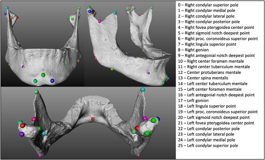
www.nature.com/scientificreports/
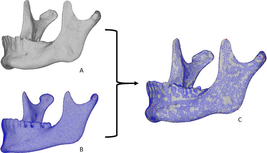
Figure 1. Illustration of the 3D dense CMF phenotyping process. A target 3D mandibular model (A) is
selected. The Meshmonk toolbox uses a non-rigid surface registration of a template mandibular mesh (B) onto
the target mandible. The red dots are the 26 anatomical landmarks used in this study and are illustrated more
clearly in Fig. 3. The result is a mapped target mandible (C) in which all landmarks are always in anatomical
correspondence across multiple subjects.
on the f ace5–7. Classic anthropometric assessment of the soft tissue component has a radiological counterpart
named cephalometric assessment. Here, the landmarks are identified on radiological data8. The distances and
angles between these identified anatomical landmarks are used to quantify facial shape.
There are two important limitations to these techniques. First of all, anthropometric and cephalometric
assessment rely on the identification of predefined anatomical landmarks by the assessor. This leaves room for
variation and error in the identification of the landmarks: is the assessor capable of identifying the landmarks
correctly and if so, are they consistent in locating the landmark? Inconsistency is one of the major pitfalls of
manual identification of landmarks8–10. Furthermore, only a limited set of landmarks are used for the quantifi-
cation of shape, underusing the rich nature of the available data in s hape1,11. This also means that the division
between what is normal and abnormal is based on a fraction of the available data.
Automatic 3D dense phenotyping is an alternative approach in quantifying facial shape. It requires capturing
and constructing a 3D model of a face or bony structure. For the soft tissues this can be done by 3D photography12
and for the skeletal structures, segmentation techniques can extract 3D skeletal surface models out of (cone beam)
computed tomography ((CB)CT) d ata13. Next, non-rigid surface registration algorithms are used to automati-
cally wrap a dense configuration of thousands of points, a mapping template, across the entire surface of the
structure of i nterest11,14. These thousands of points are called quasi-landmarks, and they replace the sparse set of
anatomical landmarks used in the classic phenotyping approach. Whenever this technique is applied to a sample
of multiple subjects, all quasi-landmarks of the mapping template are dispersed over the structure’s surface, and
they are in anatomical correspondence across those multiple subjects (Fig. 1). As an example, quasi-landmark
333 will always be located on the lateral pole of the left mandibular condyle and quasi-landmark 777 will always
be located on the center of the right tuberculum mentale. This will be the case for each 3D model of a specific
anatomical structure that is subjected to this procedure, no matter if it is derived from different patients or from
multiple CBCT scans of the same patient.
3D dense phenotyping was introduced in the early years of 200015 and since then has seen an increase in
robustness and its ability to automatically handle large-scale d atasets1,11,16. The main application of the technique
has mostly been the soft tissue facial envelope. This resulted in the development of an open-source automatic 3D
dense large-scale phenotyping toolbox called Meshmonk. The toolbox has so far only been tested and validated
on facial soft tissue shape where it has proven to be reliable and a ccurate11. The question remains how the same
techniques perform when they are applied on the underlying complex bony structures of the face. Proper assess-
ment of the reliability and accuracy of automatic 3D dense CMF phenotyping of 3D models of bony structures
is required before it is applied in a clinical or research environment. This study aimed to validate automatic 3D
dense CMF phenotyping of the human mandible using a spatially-dense non-rigid surface registration technique.
The repeated-measurement (RM) reliability and accuracy will be evaluated with classic phenotyping, using
manual landmarks, as a reference. The robustness of the technique will be assessed by applying it on a ‘normal
shape’ (unaltered mandibles) and a ‘complex shape’ (operated mandibles) sample.
Scientific Reports | (2021) 11:8532 | https://doi.org/10.1038/s41598-021-88095-w 2
Vol:.(1234567890)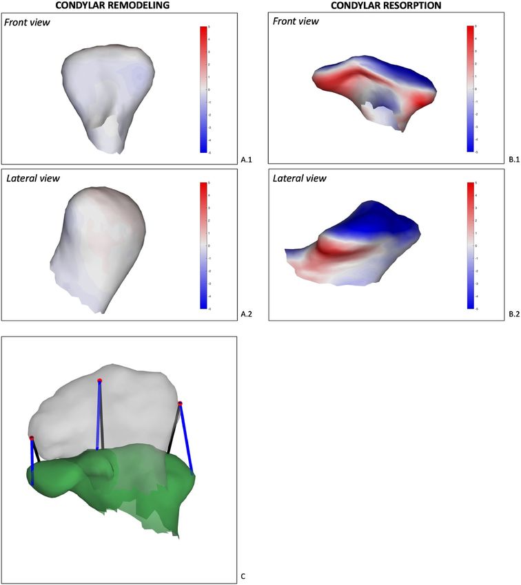
www.nature.com/scientificreports/
Figure 2. Illustration of mandibles from both samples. The unaltered mandible (A) provides a clear-cut
anatomical shape. The surgically altered mandible (B) has a more irregular outline caused by healed bone cuts
and titanium plates.
Materials and methods
Study sample. For this study, we used two samples of human mandibles. The first sample contained 30
anonymized mandibular 3D surface models, constructed out CBCT-scans taken for the virtual planning of
orthognathic surgery. This sample was labelled as the unaltered sample as the shape of the mandible is not
surgically altered. The second sample contained 20 anonymized operated mandibles that were constructed out
of 6-month follow-up CBCT scans. This sample was labelled as the operated sample due to its altered shape in
which the teeth bearing part of the mandible is displaced resulting in a more challenging and complex shape
for the non-rigid registration technique to process (Fig. 2). All scans were taken with a NewTom Vgi Evo CBCT
device (QR Verona, Verona, Italy) with the following imaging parameters FOV 24 × 19 cm, voxel size 0.3 mm3,
110 kVp and 4.3 mA. 3D surface models were constructed using a standardised and validated semi-automatic
segmentation technique17. All scans were taken for clinical purposes and ethical approval to use these scans for
research was obtained (LORTHOG Register, Department of Oral and Maxillofacial Surgery, University Hospital
Leuven, Belgium, Ethical committee approval UZ Leuven B322201526790). All methods were carried out in
accordance with relevant guidelines and regulations and informed consent was obtained from all subjects.
Phenotyping. All 3D models of the mandibles were subjected to classic phenotyping by seven oral and
maxillofacial residents, well versed in CMF anatomy and cephalometric assessment. After a calibration ses-
sion where the landmarks of interested and the landmarking tool were introduced, they identified 26 anatomi-
cal landmarks on the models using a custom-built network in MeVisLab (available: http://www.mevislab.de/)
(Fig. 3). Each resident performed the manual landmarking three times with an interval of 48 h. Automatic
phenotyping was performed using a template mandibular mesh in the Meshmonk toolbox. The template man-
dibular mesh was constructed out of 3D models derived from high resolution CT scanning of 151 dry cadaver
mandibles (MANATOMY register, Department of Oral and Maxillofacial Surgery, University Hospital Leuven,
Belgium, NH019 2019-09-03). This data was non-rigidly registered with a pre-existing mandibular template
derived from cone-beam CT of a dolescents18. The resulting meshes were co-aligned and scaled to a common size
with generalised Procrustes analysis. Averaging the co-ordinates across all 3D models resulted in the template
mesh seen in Fig. 1. The Meshmonk toolbox performs a non-rigid surface registration of the template mandibu-
lar mesh onto a target mandible after initialisation by a two-step scaled-rigid transformation of the template
onto the target as seen in Fig. 1. Firstly, it used five crudely indicated positioning landmarks (left and right lateral
condylar poles, left and right gonion and the center of the protuberans mentale) indicated on both template and
target to estimate the scaled-rigid transformation. This was further refined using a rigid iterative closest point
registration of the template onto the target also implemented in the Meshmonk toolbox. Subsequently, the non-
rigid registration is performed which alters the shape of the mapping template to match the shape of the target
mandible. The mapping template is a closed mesh consisting of 17,415 quasi-landmarks. The automatic 3D CMF
phenotyping procedure is intended to match each of those quasi-landmarks to the corresponding anatomical
position on the target mandible.
Before an accuracy assessment could be performed, the 26 anatomical landmarks used in the classic pheno-
typing approach needed to be identified in the set of 17,415 quasi-landmarks of the mapping template. For each
manual landmark (ML) identified on specific mandible by a specific observer, we identified the corresponding
automatic landmark (CAL). The mandible of interest was labelled as the target mandible, and the remaining
mandibles in the sample functioned as a training set. This leave-one-out approach was preferred to avoid train-
ing bias and resulted in a CAL for every ML identified by an observer. After each of the training mandibles had
been mapped using Meshmonk, the manually indicated landmarks on the original surface were transferred to
the mapped surface. To achieve this, a weighted sum of the three closest points on the mesh (barycentric coor-
dinates) was calculated. These barycentric coordinates were then transformed back to Cartesian coordinates to
pinpoint the location of the landmark on the mapping template. As this was done for all training mandibles, all
landmark locations were subsequently averaged, resulting in them not always ending up on the surface of the
Scientific Reports | (2021) 11:8532 | https://doi.org/10.1038/s41598-021-88095-w 3
Vol.:(0123456789)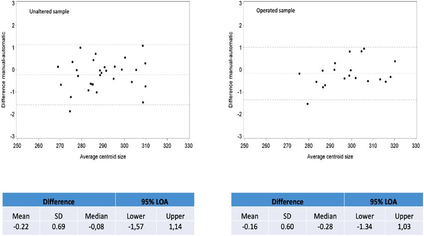
www.nature.com/scientificreports/
Figure 3. Overview of the 26 manually identified landmarks.
mapping template. This was solved by closest point surface projection in which the landmark was projected on
the surface using the shortest distance to that surface and so resulting in the identification of the corresponding
quasi-landmark. This method was slightly adapted to establish CAL for the RM reliability assessment as there is
direct comparison with the manual method, as there is in the accuracy assessment. The leave-one-out approach
was therefore omitted and all manually identified landmarks were used to train the algorithm in finding the 26
CAL among the 17,415 quasi-landmarks on the mapping template, independently for both samples.
Repeated‑measurement reliability assessment. For the validation of automatic 3D dense CMF phe-
notyping, its RM reliability was compared with the inter- and intra-observer RM reliability of classic phenotyp-
ing. Although an automated software is evidently self-consistent, the meshmonk toolbox requires identifying 5
initialisation landmarks which initiates the registration. It is this initialisation phase which still provides some
variation in automatic landmarking. Therefore, reliability of the automatic phenotyping was assessed in com-
parison to classic phenotyping. The root mean square (RMS) distance of a set of indications to the centroid of
that set was used as error statistic. The centroid is the mean position of all the points in a specific set of points.
RMS distance to the centroid was calculated as the root square of the mean of the squared Euclidean distances
of each repeated indication to the centroid of a set of indications. The smaller the RMS distance, the more
consistent a (quasi)-landmark was indicated.. Intra-observer reliability of classic phenotyping was assessed for
each of the seven observers who produced three sets of 26 landmark indications. The inter-observer reliability
of classic phenotyping was tested over the seven observers and used the averaged (n = 3) indications of the 26
landmarks by each observer. For the RM reliability assessment of automatic phenotyping, the coordinate values
of the 17,415 quasi-landmarks identified by three rounds of automatic phenotyping were used. However, to be
able to make a fair comparison between both methods, RMS distances were also calculated for the 3 sets of CAL,
as derived by the three initialisation rounds. Descriptive statistics (mean, standard deviation, minimum and
maximum RMS distance) were compared between the classic and automatic method.
Accuracy assessment. Accuracy assessment was done using the average (n = 3) ML and CAL coordi-
nate values. Three assessment approaches were used. First, for each of the 26 landmarks the Euclidean distance
between the MLs and CALs was calculated. This straightforward approach gives a good overview of how far
away MLs and CALs are located from each other. Further, we compared shape and size measurements derived
from the ML and CAL configurations. The similarity of the centroid sizes of the landmark configurations was
assessed19. Centroid size is a measure of size in geometric morphometrics and is the square root of the sum of
squared distances of all the landmarks of an object from their c entroid20. A Bland–Altman plot was given to
visualize the agreement between centroid sizes averaged over all observers. A linear mixed model with random
effects of mandible (n = 30 or n = 20) and observer (n = 7) was used to compute the contributions of mandible,
Scientific Reports | (2021) 11:8532 | https://doi.org/10.1038/s41598-021-88095-w 4
Vol:.(1234567890)www.nature.com/scientificreports/
Unaltered sample Operated sample
Mean 95% CI mean Std Min Max Mean 95% CI mean Std Min Max
Automated 0.0067 0.0043–0.0092 0.0061 0.0019 0.0217 0.0077 0.0045–0.0109 0.0079 0.0012 0.0318
Inter-operator 1.1778 0.9808–1.3748 0.4878 0.4880 2.1179 1.4046 1.1216–1.6876 0.7007 0.4807 3.4909
Intra-operator 1 0.9952 0.846–1.1444 0.3695 0.4767 1.9480 1.1175 0.8482–1.3868 0.6667 0.3282 3.3394
Intra-operator 2 1.0411 0.8751–1.2070 0.4109 0.4214 1.8050 1.0963 0.8677–1.3249 0.5659 0.4584 3.1026
Intra-operator 3 0.9125 0.7582–1.0668 0.3821 0.3348 1.9277 1.0171 0.8323–1.2019 0.4575 0.3196 2.3343
Intra-operator 4 1.1702 0.9858–1.3545 0.4565 0.5609 2.2880 1.1751 0.9038–1.4464 0.6717 0.4617 3.8427
Intra-operator 5 1.0861 0.8791–1.2931 0.5125 0.3343 2.5097 1.1996 0.9495–1.4497 0.6193 0.3510 2.5434
Intra-operator 6 0.7510 0.6609–0.8411 0.2230 0.3040 1.2313 0.8404 0.6420–1.0388 0.4913 0.2801 2.5899
Intra-operator 7 0.7669 0.6283–0.7327 0.3431 0.2929 1.9652 0.8702 0.6694–1.0710 0.4971 0.3634 2.3483
Table 1. RMS distances (mm) of repeated landmark indications to the centroid of that set of indications.
Averaged over n = 26 corresponding automatic landmarks for automatic phenotyping and n = 26 manual
landmarks for classic phenotyping. CI confidence interval, Std standard deviation, Min minimum, Max
maximum.
observer and method to the total variance of the centroid sizes. Note that the error variance in this model refers
to the contribution of method. Mixed models were fitted using PROC MIXED in SAS version 9.4. (SAS Institute
Inc., Cary, NC, USA) using restricted maximum likelihood estimation (REML). These variance components
were used to calculate the intra-class correlation coefficient (ICC), the standard error of measurement (SEM)
and the reproducibility coefficient (RC), the latter being 2.77 times the standard error of measurement (SEM).
The RC is the value below which 95% of the differences between both methods lie. Finally, the full set of inter-
landmark distances can be regarded as a very comprehensive representation of the shape of the given landmark
configuration21. For each landmarked mandible, a set of 325 distances represent the specific shape of that mandi-
ble. So, to check if the automatic and classic phenotyping achieved similar shape configurations, a generalisation
of the classic ICC for multivariate data was used on these interlandmark d istances22.
Results
Repeated‑measures reliability. Table 1 shows the error statistics for evaluating automatic and classic
phenotyping RM reliability averaged over all landmarks (26 ML and 26 CAL). Intra- and inter-observer error
statistics for each of the 26 MLs are shown in Supplementary Materials 1 and 2. The repeated-measure RMS
statistics for the 26 CAL’s are found in Supplementary Material 3. Automatic phenotyping had very low RMS dis-
tances of 0.0067 mm (unaltered sample) and 0.0077 mm (operated sample) averaged over the 26 CAL, indicative
of high consistency. The condylar region stood out as one of the most reliably mapped regions of the mandible
(Supplementary Material 4). Inter- and intra-observer error for classic phenotyping was much higher. The intra-
observer averaged (n = 26) RMS distances ranged from 0.75 to 1.17 mm in the unaltered sample and was slightly
higher in the operated sample (0.84–1.20 mm). The inter-observer averaged (n = 26) RMS distance was 1.18 mm
in the unaltered sample and 1.40 in the operated sample. The principal axes of intra- and inter-observer variation
for MLs were calculated as well (Supplementary Materials 5–8). These results showed that some of the condylar
landmarks as well as the gonial angle and chin landmarks had been susceptible to high variation when they are
manually indicated.
Accuracy. Euclidean distances. The Euclidean distance (ED) between MLs and CALs was evaluated as the
first measure of accuracy (Table 2). The average ED over all 26 landmarks was 1.40 mm for the unaltered sample
(n = 30) and 1.76 mm for the operated sample (n = 20). The most considerable differences between MLs and
CALs were found for the antegonial notches, the center of the mental foramina and the superior pole of the con-
dyle. The operated sample showed higher mean ED when compared to the unaltered sample with EDs mainly
increasing in the operated region of the mandible. The principal axes of variation between ML and CAL loca-
tions were calculated for each landmark and are shown in Supplementary Materials 9 and 10.
Centroid size comparison. Bland–Altman plots (Fig. 4) show a mean difference in centroid sizes of 0.22 mm for
the unaltered sample (n = 30, 30 mandibles, averaged centroids over observers) and 0.16 mm for the operated
sample (n = 20, 20 mandibles, averaged centroids over observers). Table 3 shows the variance components for
centroid size of the mandible (random), observer (random) and method (fixed). SAS software syntax for this
analysis can be found in Supplementary Material 11. These components were used to calculate the given ICC’s,
SEMs and RC’s in Table 3. Excellent ICC’s of > 0.99 showed an insignificant role for the method of phenotyping
(automatic vs classic). The difference in ICC between unaltered and operated mandibles was non-significant
(p = 0.5075). Reproducibility coefficients were very low, e.g. < 2 mm which is < 1% of the mean centroid size of
the mandibles in these two samples.
Shape similarity. Table 4 shows the resulting ICC for multivariate data applied on the set of 325 interlandmark
distances for each observer as well as the averaged ICC over those observers. The averaged ICC for the unal-
Scientific Reports | (2021) 11:8532 | https://doi.org/10.1038/s41598-021-88095-w 5
Vol.:(0123456789)www.nature.com/scientificreports/
Unaltered sample (n = 30) Operated sample (n = 20)
Mean Std Min Max Mean Std Min Max
Right—condylar superior pole 1.85 1.02 0.14 5.20 1.81 1.12 0.13 5.32
Right—condylar medial pole 0.76 0.40 0.15 2.49 0.93 0.62 0.19 4.27
Right—condylar lateral pole 0.81 0.45 0.09 2.74 0.93 0.60 0.22 3.07
Right—condylar most posterior point 1.66 0.94 0.06 4.83 1.81 1.15 0.17 6.52
Right—condylar fovea pterygoidea center point 0.82 0.42 0.08 2.41 0.82 0.52 0.12 3.41
Right—lowest point of the incisura 1.32 1.08 0.07 5.06 0.96 0.78 0.06 3.52
Right—most superior point of the proc. coronoideus 0.67 0.41 0.10 2.18 0.86 0.70 0.08 3.58
Right—most superior point of the lingula (spix) 1.23 0.68 0.09 3.87 2.31 1.33 0.43 6.45
Right—gonion 1.46 1.17 0.08 7.07 1.64 1.21 0.20 6.51
Right—deepest point of the antegonial notch 2.19 1.56 0.15 7.99 3.18 2.23 0.31 13.07
Right—center of foramen mentale 2.13 0.93 0.23 5.78 3.24 1.96 0.61 10.50
Right—center of Tuberculum mentale 1.68 1.25 0.12 7.91 2.11 1.63 0.15 11.94
Center—protuberans mentale 1.02 0.65 0.08 3.82 1.27 0.85 0.18 4.99
Center—center point of spina mentalis 1.34 0.86 0.14 4.99 1.58 1.13 0.09 6.21
Left—center of tuberculum mentale 1.32 0.88 0.18 4.98 1.74 1.29 0.14 12.30
Left—center foramen mentale 2.41 1.03 0.56 6.24 2.47 1.22 0.64 6.80
Left—deepest point of the antegonial notch 2.11 1.51 0.13 7.97 4.39 2.93 0.16 15.49
Left—gonion 1.69 1.06 0.22 4.97 2.32 1.40 0.07 6.04
Left—most superior point of the lingula (spix) 1.22 0.70 0.23 3.88 3.32 1.82 0.39 9.34
Left—most superior point of the proc. coronoideus 0.72 0.76 0.07 7.20 0.76 0.68 0.11 3.73
Left—lowest point of the incisura 1.42 1.24 0.12 7.92 1.18 0.96 0.13 4.50
Left—condylar fovea pterygoidea center point 1.07 0.64 0.07 3.95 0.95 0.56 0.19 4.16
Left—condylar most posterior point 1.49 0.77 0.20 4.09 1.44 0.87 0.10 4.79
Left—condylar lateral pole 0.89 0.58 0.16 3.28 0.92 0.55 0.13 2.55
Left—condylar medial pole 0.91 0.57 0.11 3.22 0.79 0.40 0.14 2.14
Left—condylar superior pole 2.12 1.35 0.13 7.56 2.01 1.13 0.16 5.14
Averaged (n = 26) 1.40 0.88 0.14 5.06 1.76 1.14 0.20 6.40
Table 2. Descriptive statistics for the Euclidean distance between the 26 MLs and CALs (mm) in the unaltered
and operated sample. Std standard deviation, Min minimum, Max maximum.
tered mandibles was 0.949 with a slightly lower 0.915 for the operated mandibles. The ICC’s for all observers
were > 0.90 in the unaltered as well as in the altered sample, indicating high similarity between shapes quantified
by classic or automatic phenotyping.
Discussion
CMF phenotyping remains an essential tool in fundamental sciences, patient diagnosis and patient follow-up. The
classic anthropometric and cephalometric approach on capturing CMF shape both have their limitations: they
are time-consuming, prone for observer error and only capture a fraction of the available shape data. Automatic
3D dense CMF phenotyping using the Meshmonk toolbox overcomes these problems. In this study, we validate
the use of this technique on meshes of human mandibles derived from CBCT.
This study assessed the RM reliability of automatic 3D phenotyping trying to answer the question: does a spe-
cific quasi-landmark always end up on the same position of the mandibular surface when the process is repeated?
Although this is to be expected by the deterministic algorithms used, the initialisation phase of the mapping by
identifying the five initialisation landmarks could introduce some variation in the mapping. The results showed
very low RMS values, especially in comparison to the manual method (> ~ 100 decrease), rendering the variation
of the mapping clinically insignificant.
Automatic phenotyping also showed good accuracy when compared to the classic approach, which still serves
as the golden standard in practice. A mean ED of 1.40 mm and 1.76 mm was found between MLs and CALs
which is in line with results from other studies on soft tissue t argets11,14,23–25. The assessment of shape similar-
ity between classic and automatic landmark configurations also showed promising results through high ICC’s
(> 0.90) for centroid size and interlandmark distances.
This study was limited by two main factors. First of all, the absence of a robust golden standard for identify-
ing anatomical landmarks makes it hard to illustrate the accuracy of automatic phenotyping. The results of the
accuracy assessment in this study should therefore be interpreted with care as they only give insights in how
automatic phenotyping compares to classic phenotyping. Secondly, we opted for 2 separate samples to assess
how the automatic phenotyping performed on a more complex shape. This however resulted in smaller sample
sizes of both groups (n = 30 and n = 20).
Scientific Reports | (2021) 11:8532 | https://doi.org/10.1038/s41598-021-88095-w 6
Vol:.(1234567890)www.nature.com/scientificreports/
Figure 4. Bland–Altman plots evaluating accuracy of automatic phenotyping by assessing agreement between
centroid sizes averaged over all observers resulting from landmark configurations of both methods. Left:
unaltered sample. Right: operated sample.
Unaltered sample Operated sample Comparison
Variance components
Jaw 144.28 168.35
Observer 0.8278 0.6861
Method 0.284 0.4401
Statistics
SEM (95% CI) 0.533 (0.498–0.573) 0.663 (0.61–0.727) p = 0.0004
RC (95% CI) 1.476 (1.379–1.588) 1.838 (1.691–2.013)
ICC (95% CI) 0.998 (0.997–0.999) 0.997 (0.995–0.999) p = 0.5075
Table 3. Variance components from a linear mixed model on centroid sizes from automatic and classic
phenotyping. Resulting variance components of method (fixed effect), jaw (random effect) and operator
(random effect) were used to calculate ICC, SEM and RC. ICC intra-class correlation, SEM standard error
of measurement, RC reproducibility, CI 95% confidence interval. For the ICC, the CI is based on the Fishers
transformation of the ICC. P-values are given for the comparison of the SEM and the ICC (both based on a Z
test).
Unaltered sample Operated sample
Observer ICC (95% CI) ICC (95% CI)
1 0.946 (0.923–0.955) 0.905 (0.861–0.931)
2 0.955 (0.938–0.962) 0.923 (0.887–0.943)
3 0.958 (0.941–0.964) 0.923 (0.887–0.943)
4 0.935 (0.913–0.945) 0.907 (0.867–0.934)
5 0.945 (0.921–0.953) 0.909 (0.857–0.938)
6 0.957 (0.940–0.965) 0.93 (0.896–0.948)
7 0.95 (0.928–0.958) 0.908 (0.861–0.934)
Mean 0.949 (0.929–0.957) 0.915 (0.874–0.939)
Table 4. ICC for the multivariate dataset of 325 interlandmark distances.
Scientific Reports | (2021) 11:8532 | https://doi.org/10.1038/s41598-021-88095-w 7
Vol.:(0123456789)www.nature.com/scientificreports/
Figure 5. Analysis of condylar remodeling using anatomical correspondence. Heat maps are displayed on the
6-month postoperative condyles of two different patients. Blue surfaces mark bone resorption and red surfaces
bone apposition with a scale in mm. Left we see a front (A.1) and lateral (A.2) view of a normal condylar
remodeling case. Right (B.1 and B.2) we see a case of condylar resorption with evident vertical bone loss marked
by the blue surface on the superior aspect of the condyle. Panel C illustrates the difference between closest point
analysis (black) and correspondent point analysis (blue) between the preoperative and postoperative condyle of
patient B for three landmarks (red dots).
Despite of these limitations, high RM reliability and good accuracy in comparison to the current clinical
standard, validate the use of automatic 3D dense CMF phenotyping on the mandible. This opens the doors for
further adaptation of this approach in science and clinical practice. Patient diagnosis and follow-up could be
facing a leap forward when this approach replaces anthropometric and cephalometric assessment. First of all,
it allows an update on the epidemiological studies to determine what a normal shape is16. This data can then
be used for enhanced patient diagnosis in which the CMF soft tissue and skeletal shape of a specific pathologi-
cal patient are compared to the norm. Only this time, the assessment is not based on a fraction of the available
Scientific Reports | (2021) 11:8532 | https://doi.org/10.1038/s41598-021-88095-w 8
Vol:.(1234567890)www.nature.com/scientificreports/
shape information, but the complete shape. Patient follow-up will also be benefit from this new approach by
establishing anatomical correspondence on 3D representations of the same or different patients26. This makes it
possible to assess surgical outcomes in CMF surgery or CMF bone remodelling. Nowadays, when comparing two
3D representations of a patient, closest point analysis is mostly used. This approach identifies the closest points
between two surfaces and interprets the distance between the points as the shape difference. It is, however, not
a given fact that the closest point is the anatomical correspondent point. 3D CMF phenotyping provides a tool
to identify anatomical correspondence on 3D models and overcome this issue.
This is showcased in Fig. 5 where we analyse remodelling of the mandibular condyle after orthognathic
surgery. After corrective surgery of the mandible, physiological remodelling of the condyle can be expected.
Sometimes, this process exceeds its physiological capacity, and a pathological volume loss of the condyles is
observed. This is accompanied by the lower jaw that falls back, reoccurrence of malocclusion and sometimes pain
in the temporomandibular joint. 3D CMF phenotyping allows for the identification of anatomical correspondent
points and allows subsequent correct quantification of how the condyle remodelled over time.
Conclusions
This study validated automatic 3D dense CMF phenotyping of the human mandible using the Meshmonk tool-
box. Excellent repeated-measures reliability and good accuracy were achieved. When combined with soft tissue
phenotyping, this approach introduces an essential improvement in quantifying CMF shape. This new application
of 3D dense automatic phenotyping will propel patient diagnosis and follow-up forward when implemented in
diagnostic and virtual surgical planning tools.
Data availability
The Meshmonk toolbox is implemented in C++ through MATLAB and the code and tutorials are available at
https://github.com/TheWebMonks/meshmonk.
Received: 3 December 2020; Accepted: 5 April 2021
References
1. Hammond, P. & Suttie, M. Large-scale objective phenotyping of 3D facial morphology. Hum. Mutat. 33, 817–825 (2012).
2. Houle, D., Govindaraju, D. R. & Omholt, S. Phenomics: The next challenge. Nat. Rev. Genet. https://doi.org/10.1038/nrg2897
(2010).
3. Farkas, L. G., Katic, M. J. & Forrest, C. R. International anthropometric study of facial morphology in various ethnic groups/races.
J. Craniofac. Surg. 16, 615–646 (2005).
4. Menéndez López-Mateos, M. L. et al. Three-dimensional photographic analysis of the face in European adults from southern Spain
with normal occlusion: Reference anthropometric measurements. BMC Oral Health 19, 196 (2019).
5. Richtsmeier, J. T., Burke Deleon, V. & Lele, S. R. The promise of geometric morphometrics. Am. J. Phys. Anthropol. 119, 63–91
(2002).
6. Reyneke, J. P. & Ferretti, C. Clinical assessment of the face. Semin. Orthod. 18, 172–186 (2012).
7. Rasmussen, C. M., Meyer, P. J., Volz, J. E., Van Ess, J. M. & Salinas, T. J. Facial versus skeletal landmarks for anterior–posterior
diagnosis in orthognathic surgery and orthodontics: Are they the same?. J. Oral Maxillofac. Surg. 78(287), e1-287.e12 (2020).
8. Pittayapat, P., Limchaichana-Bolstad, N., Willems, G. & Jacobs, R. Three-dimensional cephalometric analysis in orthodontics: A
systematic review. Orthod. Craniofac. Res. 17, 69–91 (2014).
9. Wong, J. Y. et al. Validity and reliability of craniofacial anthropometric measurement of 3D digital photogrammetric images. Cleft
Palate-Craniofac. J. https://doi.org/10.1597/06-175.1 (2008).
10. Fagertun, J. et al. 3D facial landmarks: Inter-operator variability of manual annotation. BMC Med. Imaging 14, 35 (2014).
11. White, J. D. et al. MeshMonk: Open-source large-scale intensive 3D phenotyping. Sci. Rep. 9, 6085 (2019).
12. Heike, C. L., Upson, K., Stuhaug, E. & Weinberg, S. M. 3D digital stereophotogrammetry: A practical guide to facial image acquisi-
tion. Head Face Med. 6, 18 (2010).
13. Verhelst, P. J. et al. Three-dimensional cone beam computed tomography analysis protocols for condylar remodelling following
orthognathic surgery: A systematic review. Int. J. Oral Maxillofac. Surg. https://doi.org/10.1016/j.ijom.2019.05.009 (2019).
14. Gilani, S. Z., Mian, A., Shafait, F. & Reid, I. Dense 3D face correspondence. IEEE Trans. Pattern Anal. Mach. Intell. 40, 1584–1598
(2018).
15. Hutton, T. J., Buxton, B. F., Hammond, P. & Potts, H. W. W. Estimating average growth trajectories in shape-space using kernel
smoothing. IEEE Trans. Med. Imaging 22, 747–753 (2003).
16. Weinberg, S. M. et al. The 3D facial norms database: Part 1. A web-based craniofacial anthropometric and image repository for
the clinical and research community. Cleft Palate-Craniofac. J. 53, 185–197 (2016).
17. Verhelst, P.-J. et al. Validation of a 3d CBCT-based protocol for the follow-up of mandibular condyle remodeling. Dentomaxillofac.
Radiol. https://doi.org/10.1259/dmfr.20190364 (2019).
18. Fan, Y. et al. Quantification of mandibular sexual dimorphism during adolescence. J. Anat. 234, 709–717 (2019).
19. Mitteroecker, P. & Gunz, P. Advances in geometric morphometrics. Evol. Biol. 36, 235–247 (2009).
20. Klingenberg, C. P. Size, shape, and form: Concepts of allometry in geometric morphometrics. Dev. Genes Evol. 226, 113–137 (2016).
21. Adams, D. C., Rohlf, F. J. & Slice, D. E. Geometric morphometrics: Ten years of progress following the ‘revolution’. Ital. J. Zool. 71,
5–16 (2004).
22. Shou, H. et al. Quantifying the reliability of image replication studies: The image intraclass correlation coefficient (I2C2). Cogn.
Affect. Behav. Neurosci. 13, 714–724 (2013).
23. de Jong, M. A. et al. Ensemble landmarking of 3D facial surface scans. Sci. Rep. 8, 12 (2018).
24. Guo, J., Mei, X. & Tang, K. Automatic landmark annotation and dense correspondence registration for 3D human facial images.
BMC Bioinform. 14, 232 (2013).
25. Shu Liang, Jia Wu, Weinberg, S. M. & Shapiro, L. G. Improved detection of landmarks on 3D human face data. in 2013 35th Annual
International Conference of the IEEE Engineering in Medicine and Biology Society (EMBC) 6482–6485 (IEEE, 2013). https://doi.
org/10.1109/EMBC.2013.6611039.
26. Matthews, H. S. et al. Pitfalls and promise of 3-dimensional image comparison for craniofacial surgical assessment. Plast. Reconstr.
Surg. Glob. Open 8, e2847 (2020).
Scientific Reports | (2021) 11:8532 | https://doi.org/10.1038/s41598-021-88095-w 9
Vol.:(0123456789)www.nature.com/scientificreports/
Author contributions
H.P., P.C. R.J., C.P. H.M. and P.V designed and facilitated the experiment and study. L.V., F.V., D.M., T.C., O.D.,
M.S., P.V. and H.M landmarked all 3D models and participated in the landmarking experiment. H.M., S.F. and
P.V. performed the statistical analysis. E.S., H.P., P.C., C.P. and R.J. provided input throughout the analysis and
writing process. P.V. and H.M. wrote the manuscript. All authors revised the manuscript.
Competing interests
The authors declare no competing interests.
Additional information
Supplementary Information The online version contains supplementary material available at https://doi.org/
10.1038/s41598-021-88095-w.
Correspondence and requests for materials should be addressed to P.-J.V.
Reprints and permissions information is available at www.nature.com/reprints.
Publisher’s note Springer Nature remains neutral with regard to jurisdictional claims in published maps and
institutional affiliations.
Open Access This article is licensed under a Creative Commons Attribution 4.0 International
License, which permits use, sharing, adaptation, distribution and reproduction in any medium or
format, as long as you give appropriate credit to the original author(s) and the source, provide a link to the
Creative Commons licence, and indicate if changes were made. The images or other third party material in this
article are included in the article’s Creative Commons licence, unless indicated otherwise in a credit line to the
material. If material is not included in the article’s Creative Commons licence and your intended use is not
permitted by statutory regulation or exceeds the permitted use, you will need to obtain permission directly from
the copyright holder. To view a copy of this licence, visit http://creativecommons.org/licenses/by/4.0/.
© The Author(s) 2021
Scientific Reports | (2021) 11:8532 | https://doi.org/10.1038/s41598-021-88095-w 10
Vol:.(1234567890)You can also read