BETA DISTRIBUTED CREDIT SCORE - ESTIMATION OF ITS J-DIVERGENCE
←
→
Page content transcription
If your browser does not render page correctly, please read the page content below
The 7th International Days of Statistics and Economics, Prague, September 19-21, 2013

  BETA DISTRIBUTED CREDIT SCORE - ESTIMATION OF
                ITS J-DIVERGENCE
                                         Martin Řezáč

Abstract
It is known, that Beta distribution could provide a reasonable approximation of distribution of
a credit scores, which are the outcome of credit scoring models, i.e. models which are used to
determine the probability of default (i.e. when the client fails to meet his or her credit
obligations). Credit scoring models are used in practice in the majority of decisions related to
the granting of credits, and are thus inherently part of the majority of processes (approval,
enforcement, commercial, etc.) in the financial sector. Besides Gini coefficient or K-S
statistic, J-divergence (also called Information value) is widely used to assess discriminatory
power of credit scoring models. However, empirical estimator using deciles of scores, which
is the common way how to compute the J-divergence, may lead to strongly biased results. The
main aim of this paper is to describe properties of alternative, both parametric and non-
parametric, estimators of J-divergence for credit scoring models with Beta distributed scores.
As we show, the parametric and ESIS estimators are much more appropriate to use
considering both the bias and mean squared error. Indeed, better estimator leads to better
assessment of models, what may lead to better credit scoring models used in practice.

Key words: J-divergence, Information Value, Credit Scoring, Beta Distribution.

JEL Code: E51, C14, C63

Introduction
J-divergence is one of the frequently used ways of describing the difference between two
probability distributions. When considering the quality (discriminatory power) of a
classification model, maximally different conditional probability distributions is exactly what
one aims to. Thus the J-divergence is very suitable, and also widely used, to assess the quality
of classification models. It is also known under the name of Information value, in the case of
its use for the purpose of scoring models, e.g. credit scoring models that are used to determine
the probability of default (i.e. when the client fails to meet his or her credit obligations).
Credit scoring models are used in practice in the majority of decisions relating to the granting

                                               1182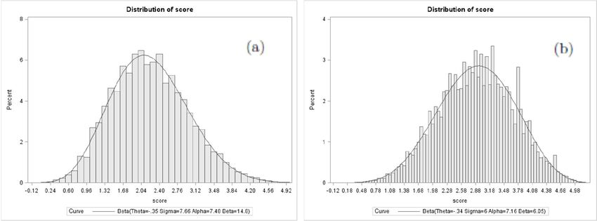
The 7th International Days of Statistics and Economics, Prague, September 19-21, 2013
of loans, and are inherently part of the processes (approval, collection, sales, etc.) in the
financial sector. Development methodology of credit scoring models and methods for
assessing their quality can be found in articles such as Hand and Henley (1997), Thomas
(2000) Vojtek and Kočenda (2006) or Crook et al. (2007) and books like Anderson (2007) or
Thomas (2009).
This paper deals primarily with the J-divergence, which is one of the widely used
indices (next to the Gini index and KS statistics, see Crook et al. (2007) or Řezáč and Řezáč
(2011) for details) for assessment of the quality of credit scoring models. Usually it is
calculated by a discretization of the score into intervals using deciles with the requirement for
a nonzero number of observations in all intervals. However, this could lead to strongly biased
estimate of the J-divergence. As an alternative method to the empirical estimates one can use
the kernel smoothing theory, which allows to estimate unknown densities and consequently,
using some numerical method for integration, to estimate value of the J-divergence. Another
alternative is the empirical estimates with supervised interval selection (ESIS) proposed and
discussed in Řezáč (2011). Details connected to the kernel estimates and a discussion
concerning both these approaches one can find there as well.
The main objective of this paper is to describe the behaviour of the J-divergence
estimates of credit scoring models with Beta distributed score. The second and the third
chapter deal with the methodology of these estimates, including algorithms or reference to the
relevant literature. The fourth chapter is then devoted to justify appropriateness of Beta
distribution on a real data, though the choice of this distribution type was justified in the
literature, e.g. in Jankowitsch et al. (2007) or Moraux (2010). Furthermore, this chapter is
devoted to computation of the J-divergence on the real data. There are also, using a simulation
study, discussed the properties of estimates described within the paper.
1 J-divergence for Beta distributed score
Jeffrey divergence (J-divergence) of two random variables X0 and X1 with densities f0(x) and
f1(x) is defined as symmetrised Kullback-Leibler divergence, i.e.
f ( x)
D J ( X 0 , X 1 ) D KL ( X 0 : X 1 ) D KL ( X 1 : X 0 ) f
0 ( x ) f1 ( x ) ln 0 dx,
f1 ( x )
(1)
where Kullback-Leibler divergence DKL ( X 0 : X1 ) is given by
f ( x)
D KL ( X 0 : X 1 ) f
0 ( x ) ln 0 dx.
f1 ( x )
(2)
1183The 7th International Days of Statistics and Economics, Prague, September 19-21, 2013
Consider thus two random variables X0 and X1 representing suitably transformed
outputs of the credit scoring model for bad (clients in default) and good clients. Let these
random variables be Beta distributed with densities f0(x) and f1(x) defined by
1
( x 0 ) 0 1 ( 0 0 x) 0 1 for 0 x 0 0
f 0 ( x) B ( 0 , 0 ) 0 0 0 1 (3)
0 for x 0 or x 0 0
1
( x 1 ) 1 1 ( 1 1 x) 1 1 for 1 x 1 1
f1 ( x) B ( 1 , 1 ) 1 1 1 1 (4)
0 for x 1 or x 1 1 .
x i
It is easy to show that the transformations y , i = 0,1, convert random variables X0
i
and X1 to random variables Y0 a Y1 with densities
1
y 0 1 (1 y ) 0 1 for 0 y 1
g 0 ( y ) B( 0 , 0 ) (5)
0 otherwise,
1
y 1 1 (1 y ) 1 1 for 0 y 1
g1 ( y ) B (1 , 1 ) (6)
0 otherwise.
For such distributed random variables one can find analytical expression of the Kullback-
Leibler divergence, and hence also of the J-divergence. We get therefore
DJ (Y0 , Y1 ) (1 0 ) (1 ) ( 0 ) ( 1 0 ) ( 1 ) ( 0 )
(7)
(1 0 1 0 ) ( 0 0 ) ( 1 1 ) ,
where (t ) is the digamma function. See Gradshtein and Ryzhik (1965) or Medina and Moll
(2009) for details about the digamma function. The J-divergence can also be calculated by
approximative formula using the relationship (t ) ln(t 0,5) , see Johnson, Kotz and
Balakrishnan (1995). Then it holds
0,5 1 0 0,5 1 0 0,5 1 0 1 0
DJ (Y0 , Y1 ) ln 1 1 0 0
. (8)
0 0,5 0 0,5 1 1 0,5
1184The 7th International Days of Statistics and Economics, Prague, September 19-21, 2013
Furthermore, one still needs to estimate the parameters 0 ,1 , 0 and 1 for the practical
estimation of the J-divergence. Typically, this is done using the MLE estimates. Those are
available for example in Univariate procedure in SAS system. Computational schemes of
these MLE estimates can then be found in Johnson, Kotz a Balakrishnan (1995). Overall, we
obtain the parametric estimates by this procedure.
One point has to be mentioned here. The J-divergence is not generally invariant with
respect to transformations. Indeed, this holds for transformations used for converting four-
parameters Beta distributed variables given by (3) and (4) to two-parameters Beta distributed
variables given by (5) and (6). Nevertheless, when comparing the discriminative power of
several credit scoring models on the same data, then this property (disadvantage) does not
matter. And what is quite important, estimation of parameters in (3) and (4) and consequent
computation of the J-divergence is quite complicated. From this perspective, it seems to be
appropriate to use parametric estimate given by (7) or (8).
2 Non-parametric estimates of J-divergence
In practice, the most commonly used non-parametric estimators of the J-divergence are the
empirical estimates. These are based on the idea of replacing unknown densities by empirical
estimates of these densities, de facto using appropriate relative frequencies. Let's have n0
score values s 0i , i 1,, n0 for bad clients and n1 score values s1i , i 1,, n1 for good clients
and denote L (resp. H) as the minimum (resp. maximum) of all values.
Let's divide the interval [L, H] up to r subintervals [q0, q1], (q1, q2],…,(qr-1, qr], where
q 0 L 1, q r H 1, q i , i 1, , r 1 and q i , i 1, , r 1 are suitable border points, e.g.
appropriate quantiles of score of all clients. Set
n0
n0 j I ( s 0i (q j 1 , q j ] )
i 1
n1 (9)
n1 j I ( s1i (q j 1 , q j ] ) j 1, , r
i 1
observed counts of bad or good clients in each interval. Denote fˆIV ( j ) the contribution to the
information value on jth interval, calculated by
n1 n0 n1 n0
fˆIV ( j ) j j ln j , j 1,, r . (10)
n
1 n0 n0 j n1
The empirical estimate of the J-divergence is given by
1185The 7th International Days of Statistics and Economics, Prague, September 19-21, 2013
r
Dˆ J fˆIV ( j ) . (11)
j 1
A special case is the decile estimate which uses scores of all clients and r = 10 to determine
the boundaries of the interval qi. Further algorithms are then e.g. ESIS, see Řezáč (2011),
ESIS1, see Řezáč and Koláček (2011), or ESIS2, see Řezáč (2012).
Further possible way how to estimate the J-divergence is the usage of the theory of
kernel density estimates. For given M+1 equidistant point of the score L x0 , x1 , , xM H
we have
M 1
H L~ ~ ~
Dˆ J f IV ( L) 2 f IV ( xi ) f IV ( H ) , (12)
2M i 1
~
where f IV ( xi ) are estimated contributions to the J-divergence given by appropriate kernel
estimates of the unknown densities of bad and good clients’ scores. See Řezáč (2011) for
more details.
3 Results
The logical question is why to consider just the Beta distribution. Some arguments were given
in Jankowitsch et al. (2007) and Moraux (2010). Furthermore, the answer can be found in the
following Figures 1 and 2 and Tables 1 and 2, obtained using the SAS UNIVARIATE
procedure. There was some real data provided by a financial institution including output of a
credit scoring model (inverse logit transformation of 1 minus the probability of default) and a
good/bad indicator of the client. The data range was 176,878 observations, see Řezáč a Řezáč
(2011) for more details.
Fig. 1: Fitted Beta distributions of scores. a) for bad, b) for good clients.
Source: Own construction.
1186The 7th International Days of Statistics and Economics, Prague, September 19-21, 2013
From the Figure 1 (fitted Beta densities and histograms) and especially from the
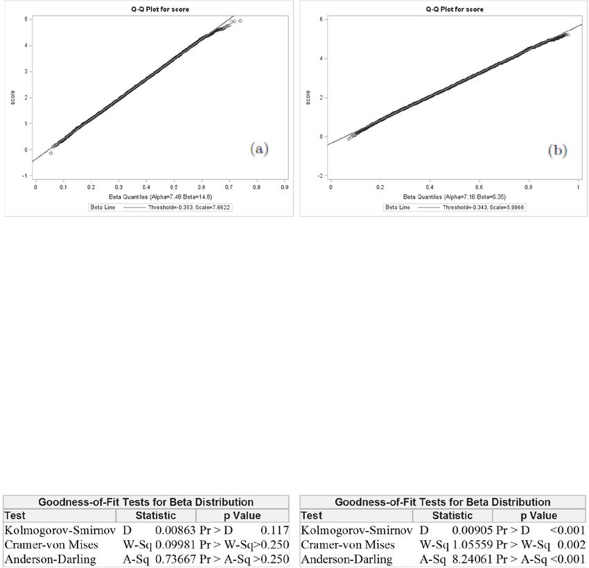
Figure 2 (Q-Q charts) it is obvious that the choice of the Beta distribution was appropriate.
Fig. 2: Q-Q charts for fitted Beta distributions of scores. a) for bad, b) for good clients.
Source: Own construction
The following Table 1 contains the results of goodness of fit (GoF) tests of the
examined data. In case of bad clients’ score, all considered tests did not reject the hypothesis
of a Beta distribution. On the other hand, in case of good clients’ score there was
approximately tenfold growth of test statistics for the Cramer-von Mises and Anderson-
Darling tests but the test statistics of the Kolmogorov-Smirnov test remained at approximately
the same value. Overall, all three tests rejected the hypothesis of a Beta distributed score in
the case of good clients’ score.
Tab. 1: Goodness of fit tests of scores. a) for bad, b) for good clients.
(a) (b)
Source: Own construction.
The problem (results of GoF tests for good clients’ score) lies in the very large range
(approximately 160,000 observations) of data. It is commonly known that with a large data
set, the GoF test becomes very sensitive to even very small, inconsequential departures from a
distribution. Due to this phenomenon it is recommended (for large data set) to follow the
result of Q-Q chart rather than results of GoF tests. Even if we did not want to follow this
recommendation, it applies that when performing the same tests (more specifically, we did
one thousand tests) on a random sample of good clients’ score comprising 10% of the original
1187The 7th International Days of Statistics and Economics, Prague, September 19-21, 2013
number of observations we got approximately the same results as for bad clients’ score (even
with higher p-values for all three tests). Overall, we stated that scores of bad and good clients
could be considered Beta distributed.
Table 2 contains parameters of the fitted Beta distributions. The most striking
difference between good and bad clients’ score is given by the parameter beta (14.8 vs. 6.05)
and the parameter sigma (7.66 vs. 5.99).
Tab. 2: Parameters of Beta distributed scores. a) for bad, b) for good clients.
(a) (b)
Source: Own construction.
The following Table 3 shows values of DJ estimated by the algorithms mentioned
above. The last line contains the parameter estimate given by (7) with MLE estimates of
parameters. As the best non-parametric estimate seems to be the value 3.117 given by the
algorithm ESIS1.
Tab. 3: Estimates of DJ .
DJ
decil 2.508551
kern 2.797372
esis 2.945658
esis1 3.117013
esis2 2.967163
param 3.403594
Source: Own construction.
The question, however, is the general behaviour of these algorithms. A very common
way to assess the quality / properties of some parameter estimates or statistics are bias (bias)
and mean square error (MSE), defined by
bias E Dˆ J DJ , (13)
2
MSE E Dˆ J D .
(14)
1188The 7th International Days of Statistics and Economics, Prague, September 19-21, 2013
The following Figures 3 and 4 show the properties of these algorithms from this perspective.
Simulation study leading to these results was carried out as follows. We consider n clients,
n pB bad and n (1 pB ) good (pB is the relative frequency of bad clients). In our case we
choose pB = 0.1, which is the closest to the aforementioned real data. Furthermore, we
consider the parameters of Beta distribution resulting the value DJ = 1.00 and 2.25. Range of
data sample we choose n = 1000 and n = 100 000. First, we generate scores of bad and good
clients, depending on the selected parameters. Then we calculate all of the aforementioned
estimates. This process was repeated one thousand times. Mean values for the bias and the
MSE are then calculated as the arithmetic means.
Fig. 3: Bias of estimates of D̂ J for Beta distributed of scores.
Source: Own construction.
Fig. 4: Logarithm of MSE of estimates of D̂J for Beta distributed of scores.
Source: Own construction.
1189The 7th International Days of Statistics and Economics, Prague, September 19-21, 2013
From the Figures 3 and 4 it is apparent that the decile estimate is significantly biased,
specifically undervalued. The value of log MSE became quite quickly stabilized and with
increasing number of observations did not fall. Overall, this estimate is thus not very suitable.
In contrast, algorithms ESIS1 and ESIS2 led in the case of a weaker model (DJ = 1.00) to
almost unbiased estimate. For a stronger model (DJ = 2.25) are their properties worse.
However, they were the best of all considered methods of estimating DJ.
Conclusion
The aim of this paper was to describe properties of the selected estimates of J-divergence
(also called Information value) of credit scoring models with Beta distributed scores. It was
given a formula for the theoretical value of the J-divergence assuming this type of
distribution. Its knowledge enabled the both compute parametric estimates, but also to assess
the quality of non-parametric estimates. On real data it was presented an estimate of the J-
divergence. In addition, properties of aforementioned estimates have been demonstrated on
simulated data from the Beta distribution. Namely, they were the bias and the MSE for the
data ranges from 1000 to 100 000. It quite obviously turned out the weaknesses of traditional
decile empirical estimation. Conversely, it seemed that the algorithms ESIS1 and ESIS2 were
good estimates of J-divergence with Beta distributed score.
References
Anderson, R. The Credit Scoring Toolkit: Theory and Practice for Retail Credit Risk
Management and Decision Automation. Oxford: Oxford University Press, 2007.
Crook J.N., Edelman D.B., Thomas L.C. Recent developments in consumer credit risk
assessment. European Journal of Operational Research, 183(3), pp.1447–1465, 2007.
Gradstein, I.S. and Ryzhik, I.M. Tables of integrals, sums, series and products. New York
and London: Academic Press, 1965.
Hand, D.J. and Henley, W.E. Statistical Classification Methods in Consumer Credit Scoring:
a review. Journal. of the Royal Statistical Society, Series A, 160,No.3, pp. 523-541, 1997.
Jankowitsch, R., Pichler, S., Schwaiger, W.S.A. Modelling the economic value of credit
rating systems. Journal of Banking & Finance, 31, pp. 181–198, 2007.
Johnson, N. L., Kotz, S., Balakrishnan, N. Continuous Univariate Distributions, volume 2,
2nd edition. New York: Wiley, 1995.
1190The 7th International Days of Statistics and Economics, Prague, September 19-21, 2013
Medina, L.A. and Moll, V. H. The integrals in Gradshteyn and Ryzhik. Part 10: The digamma
function. Scientia, Series A: Mathemaical Sciences 17, pp. 45-66, 2009.
Moraux, R. Sensitivity Analysis of Credit Risk Measures in the Beta Binomial Framework.
The Journal of Fixed Income, 19(3), pp. 66-76, 2010.
Řezáč, M. Advanced empirical estimate of information value for credit scoring models. Acta
Universitatis Agriculturae et Silviculturae Mendelianae Brunensis LIX (2), s. 267-273,
2011.
Řezáč, M. Information Value Estimator for Credit Scoring Models. Proceedings of ECDM
2012, Lisboa, s. 188-192, 2012.
Řezáč, M. and Koláček, J. Computation of Information Value for Credit Scoring Models.
Workshop of the Jaroslav Hájek Center and Financial Mathematics in Practice I, Book of
short papers, pp. 75-84, 2011.
Řezáč, M. and Řezáč, F. How to Measure the Quality of Credit Scoring Models. Finance a
úvěr - Czech Journal of Economics and Finance 61 (5), pp. 486-507, 2011.
Thomas, L.C. A survey of credit and behavioural scoring: forecasting financial risk of lending
to consumers. International Journal of Forecasting 16 (2), pp. 149-172, 2000.
Thomas, L.C. Consumer Credit Models: Pricing, Profit, and Portfolio. Oxford: Oxford
University Press, 2009.
Vojtek M, Kočenda E. Credit Scoring Methods. Finance a úvěr-Czech Journal of Economics
and Finance, 56(3-4), pp.152–167, 2006.
Contact
Martin Řezáč
Masaryk University, Faculty of Science, Department of Mathematics and Statistics
Kotlářská 2
611 37 Brno
mrezac@math.muni.cz
1191You can also read