Birds Sings Detection in Chingaza National Park Records Using Orthogonal Decomposition.
←
→
Page content transcription
If your browser does not render page correctly, please read the page content below

Birds Sings Detection in Chingaza
National Park Records Using Orthogonal
            Decomposition.

                         by
             Carlos Andrés Posada

                        at the

       PONTIFICIA UNIVERSIDAD JAVERIANA CALI

              FACULTY OF ENGINEERING
DEPARTMENT OF ELECTRICAL ENGINEERING AND COMPUTER
                     SCIENCE

                  November 13, 2014
Birds Sings Detection in Chingaza
National Park Records Using Orthogonal
            Decomposition.

                                    by
                   Carlos Andrés Posada

   A Thesis Presented in Fulfillment of the Requirements for the Degree of
                         Electronic Engineer

                                 Adviser
                           Luis E. Tobón

                                   at the

        PONTIFICIA UNIVERSIDAD JAVERIANA CALI

              FACULTY OF ENGINEERING
DEPARTMENT OF ELECTRICAL ENGINEERING AND COMPUTER
                     SCIENCE

                           November 13, 2014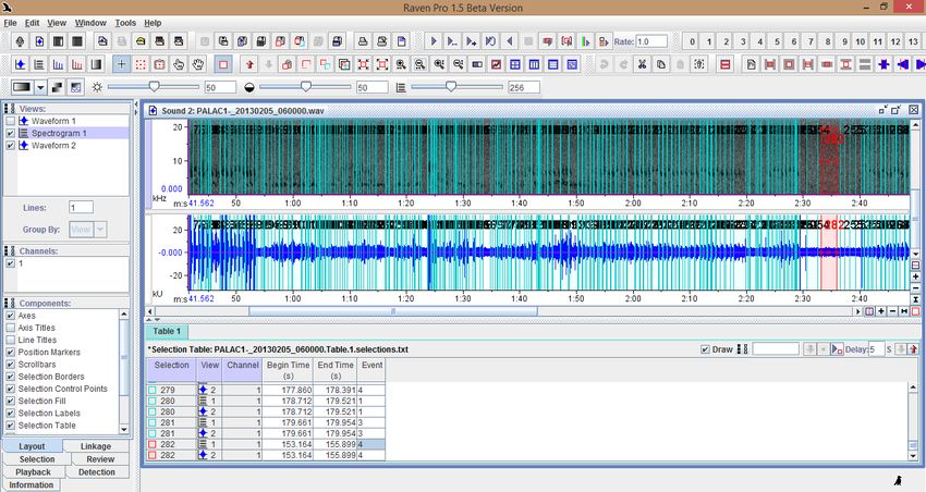
Abstract

The importance of studies of natural conservation, as well as the new technologies in sensing
and communications, are generating large amounts of information that should be analyzed.
In Colombia the Alexander von Humboldt institute has over 1000 hours of audio record coming
from different Colombian ecosystems such as Chingaza Natural Parck, Sierra Nevada de Santa
Marta, Magdalena Medio, Gorgona and Chocó. These records allow to perform studies on
conservation of ecosystems and species. Hence, it requires new methods and systems to
reduce the cost of data processing. On the other hand, birds presence are good indicator
of the state of ecosystems because they are distributed over a wide range of landscapes,
and there are large amount of studies about their behavior. Additionally, it is important to
mention, the fact that Colombia is currently the country with the highest number of bird
species in the world. All these aspects demand the development of automated systems to
detect vocalizations of birds in audio records coming from Colombian ecosystems.

This work presents the design and test of a system for detection of birds vocalization on
Chingaza Natural Park records. This system uses a signal decomposition method that uses
orthogonal families as basis functions. The designed detector has a good performance, with
successful detection of vocalizations of birds over 80% and only 18% of false alarms. Addi-
tionally, this work presents an energy consumption analysis for three different distributions
of detection algorithms it shows the potential use for species classification and soundprint
ecosystem characterization.

Keywords: Natural Conservation, Signals Decomposition, Orthogonal Polynomials, Detec-
tors Combination, Binary Detector Theory, Bird Classification, Sound Print, Distributive
Algorithms, Energy Consumption.
Contents

Abstract                                                                                                                 i

List of Figures                                                                                                         iv

List of Tables                                                                                                          vi

List of Abbreviations                                                                                                   1

1 Introduction                                                                                                          1

2 Overview                                                                                                              3
  2.1 Problem Formulation . . . . . . . . . . . . . . . . . . . . . . . . . . . . . . . .                               3
  2.2 Research Hypothesis. . . . . . . . . . . . . . . . . . . . . . . . . . . . . . . . .                              4

3 Objectives                                                                                                            5
  3.1 General Objective . . . . . . . . . . . . . . . . . . . . . . . . . . . . . . . . .                               5
  3.2 Specific Objective . . . . . . . . . . . . . . . . . . . . . . . . . . . . . . . . . .                            5

4 Scope                                                                                                                 6

5 Orthogonal Polynomial Decomposition                                                                                    7
  5.1 Orthogonality and Orthonormality in Continuous          Time      .   .   .   .   .   .   .   .   .   .   .   .    7
  5.2 Polynomial Families. . . . . . . . . . . . . . . . .    . . . .   .   .   .   .   .   .   .   .   .   .   .   .    8
      5.2.1 Chebyshev Polynomial . . . . . . . . . . .        . . . .   .   .   .   .   .   .   .   .   .   .   .   .    9
      5.2.2 Legendre Polynomials. . . . . . . . . . . .       . . . .   .   .   .   .   .   .   .   .   .   .   .   .   10
      5.2.3 Hermite Polynomials. . . . . . . . . . . .        . . . .   .   .   .   .   .   .   .   .   .   .   .   .   11
      5.2.4 The Harmonics Functions. . . . . . . . . .        . . . .   .   .   .   .   .   .   .   .   .   .   .   .   12
  5.3 Orthogonality in Discrete Time. . . . . . . . . . .     . . . .   .   .   .   .   .   .   .   .   .   .   .   .   12
      5.3.1 Metric of Orthogonality. . . . . . . . . . .      . . . .   .   .   .   .   .   .   .   .   .   .   .   .   13
  5.4 Signal Decomposition . . . . . . . . . . . . . . .      . . . .   .   .   .   .   .   .   .   .   .   .   .   .   14
  5.5 Signals Reconstruction . . . . . . . . . . . . . . .    . . . .   .   .   .   .   .   .   .   .   .   .   .   .   14
  5.6 Thresholding . . . . . . . . . . . . . . . . . . . .    . . . .   .   .   .   .   .   .   .   .   .   .   .   .   15
      5.6.1 Total Threshold. . . . . . . . . . . . . . .      . . . .   .   .   .   .   .   .   .   .   .   .   .   .   15
      5.6.2 Columns Thresholding . . . . . . . . . . .        . . . .   .   .   .   .   .   .   .   .   .   .   .   .   15
  5.7 Reconstruction Error . . . . . . . . . . . . . . . .    . . . .   .   .   .   .   .   .   .   .   .   .   .   .   15
  5.8 Energy Concentration . . . . . . . . . . . . . . .      . . . .   .   .   .   .   .   .   .   .   .   .   .   .   16
  5.9 Examples . . . . . . . . . . . . . . . . . . . . . .    . . . .   .   .   .   .   .   .   .   .   .   .   .   .   16

                                                ii
Contents iii
6 Resolution Analysis 25
6.1 Empirical Procedures . . . . . . . . . . . . . . . . . . . . . . . . . . . . . . . . 25
7 Detectors Design 28
7.1 Detection Theory. . . . . . . . . . . . . . . . . . . . . . . . . . . . . . . . . . 28
7.2 Coefficient Energy Distributions . . . . . . . . . . . . . . . . . . . . . . . . . 30
7.2.1 Data Histograms and Rayleigh’s Approach. . . . . . . . . . . . . . . . 31
7.2.2 Coefficients Selection . . . . . . . . . . . . . . . . . . . . . . . . . . . . 32
7.3 Theoretical ROCs . . . . . . . . . . . . . . . . . . . . . . . . . . . . . . . . . 33
7.4 Detectors Combination . . . . . . . . . . . . . . . . . . . . . . . . . . . . . . . 34
7.4.1 Single Coefficient Detector . . . . . . . . . . . . . . . . . . . . . . . . . 34
7.4.2 Summation Detector . . . . . . . . . . . . . . . . . . . . . . . . . . . . 35
7.4.3 Product Detector . . . . . . . . . . . . . . . . . . . . . . . . . . . . . . 36
7.4.4 Majority Vote Detector . . . . . . . . . . . . . . . . . . . . . . . . . . 37
7.4.5 Cascade Detector . . . . . . . . . . . . . . . . . . . . . . . . . . . . . . 38
8 Algorithm Distributions 40
8.1 Mote Features. . . . . . . . . . . . . . . . . . . . . . . . . . . . . . . . . . . . 40
8.2 Communication Protocol . . . . . . . . . . . . . . . . . . . . . . . . . . . . . . 41
8.3 Distributions Design. . . . . . . . . . . . . . . . . . . . . . . . . . . . . . . . . 42
9 Results 44
9.1 Decomposition Results . . . . . . . . . . . . . . . . . . . . . . . . . . . . . . . 44
9.2 Detectors Results. . . . . . . . . . . . . . . . . . . . . . . . . . . . . . . . . . 45
9.3 Distributions Results. . . . . . . . . . . . . . . . . . . . . . . . . . . . . . . . 46
9.4 Bird Species Characterization . . . . . . . . . . . . . . . . . . . . . . . . . . . 47
9.5 Ecosystems Characterization . . . . . . . . . . . . . . . . . . . . . . . . . . . 48
10 Conclusions 51
11 Future Work 53
A User Manual 55
B IV Ornithological Colombian Congress Participation 58
C STSIVA Paper 60
Bibliography 66List of Figures
5.1 Chebyshev Polynomials of Degree 0, 2, 4, 6. . . . . . . . . . . . . . . . . . . . 9
5.2 Chebyshev Polynomials of Degree 0, 1 ,2, 3. . . . . . . . . . . . . . . . . . . . 10
5.3 Hermite polynomials of degree 3, 4 ,5, 6. . . . . . . . . . . . . . . . . . . . . . 11
5.4 Harmonic functions n= 0, 1 ,2, 3. . . . . . . . . . . . . . . . . . . . . . . . . . 12
5.5 Frequency Modulated Signal in (a) Time Domain and (b) Frequency Domain. 17
5.6 Frequency modulate Signal Decomposition Using: (a) Legendre Polynomials,
(b) Harmonic Functions, (c) Chebyshev Polynomials and (d) Hermite Polyno-
mials. . . . . . . . . . . . . . . . . . . . . . . . . . . . . . . . . . . . . . . . . 18
5.7 Interference Signal in (a) Time Domain and (b) Frequency Domain. . . . . . 19
5.8 Interference Signal Decomposition Using: (a) Legendre Polynomials, (b) Har-
monic Functions, (c) Chebyshev Polynomials and (d) Hermite Polynomials. . 20
5.9 Acropternis orthonyx Sing in (a) Time Domain and (b) Frequency Domain. . 21
5.10 Acropternis orthonyx Sing Decomposition Using: (a) Legendre Polynomials,
(b) Harmonic Functions, (c) Chebyshev Polynomials and (d) Hermite Polyno-
mials. . . . . . . . . . . . . . . . . . . . . . . . . . . . . . . . . . . . . . . . . 22
5.11 Chingaza Record (a) Time Domain and (b) Frequency Domain. . . . . . . . . 23
5.12 Chingaza Record Decomposition Using: (a) Legendre Polynomials, (b) Har-
monic Functions, (c) Chebyshev Polynomials and (d) Hermite Polynomials. . 24
6.1 Reconstruction error using different value for N and Lp for: (a) Legendre
Polynomials, (b) Harmonic Functions, (c) Chebyshev Polynomials and (d)
Hermite Polynomials. . . . . . . . . . . . . . . . . . . . . . . . . . . . . . . . 26
6.2 Representation using resolution 10x11, 40x41,8x81 for: (a) Legendre Polyno-
mials, (b) Harmonic Functions, (c) Chebyshev Polynomials and (d) Hermite
Polynomials. . . . . . . . . . . . . . . . . . . . . . . . . . . . . . . . . . . . . 27
7.1 Probability Density Function for i-th Coefficient. . . . . . . . . . . . . . . . . 29
7.2 Probability of Detection . . . . . . . . . . . . . . . . . . . . . . . . . . . . . . 30
7.3 Probability of False Alarm . . . . . . . . . . . . . . . . . . . . . . . . . . . . . 30
7.4 Record File Split. . . . . . . . . . . . . . . . . . . . . . . . . . . . . . . . . . . 31
7.5 Coefficient i-th Histograms. . . . . . . . . . . . . . . . . . . . . . . . . . . . . 31
7.6 (a) Histograms for i-th coefficient, (b) Corresponding pdfs for i-th coefficient. 32
7.7 Sigma Value for Each Coefficient of Each Data Type in: (a) Harmonic Func-
tions and (b) Legendre Polynomials. . . . . . . . . . . . . . . . . . . . . . . . 33
7.8 Single Coefficients ROC for: (a) Harmonics Ideal, (b) Harmonics Exp, (d)
Legendre Ideal and (d) Legendre Exp. . . . . . . . . . . . . . . . . . . . . . . 35
7.9 Summation Detector ROCs for: (a) Harmonic Functions and (b) Legendre
Polynomials. . . . . . . . . . . . . . . . . . . . . . . . . . . . . . . . . . . . . 36
ivList of Figures v
7.10 Product Detector ROCs for: (a) Harmonic Functions and (b) Legendre Poly-
nomials. . . . . . . . . . . . . . . . . . . . . . . . . . . . . . . . . . . . . . . . 37
7.11 Majority Vote Detector ROCs for: (a) Harmonic Functions and (b) Legendre
Polynomials. . . . . . . . . . . . . . . . . . . . . . . . . . . . . . . . . . . . . 38
7.12 Cascade Detector. . . . . . . . . . . . . . . . . . . . . . . . . . . . . . . . . . 38
7.13 Theoretical and Real ROC for Cascade Detector using (a) Harmonics Function
and (b) Legendre Functions. . . . . . . . . . . . . . . . . . . . . . . . . . . . . 39
8.1 (a) TDMA Data Packages, (b) TDMA Control Package (c) CDMA Package. . 42
8.2 (a) Distribution 1, (b) Distribution 2 (c) Distribution 3. . . . . . . . . . . . . 43
9.1 (a) Polynomial Decomposition, (b) Energy Distribution. . . . . . . . . . . . . 47
9.2 Energy Distribution from four Bird Species. . . . . . . . . . . . . . . . . . . . 48
9.3 Chingaza Record Distribution of February 5th, 2013 at 6:00 am. . . . . . . . 49
9.4 Chingaza Day distributions for: 04 February, 05 February and 06 February of
2013. . . . . . . . . . . . . . . . . . . . . . . . . . . . . . . . . . . . . . . . . . 50
11.1 Spectral features for classification. . . . . . . . . . . . . . . . . . . . . . . . . 54
A.1 Main Window . . . . . . . . . . . . . . . . . . . . . . . . . . . . . . . . . . . . 55
A.2 Load File . . . . . . . . . . . . . . . . . . . . . . . . . . . . . . . . . . . . . . 56
A.3 Signal Decomposition. . . . . . . . . . . . . . . . . . . . . . . . . . . . . . . . 56
A.4 Detecting Vocalizations of Birds. . . . . . . . . . . . . . . . . . . . . . . . . . 57
A.5 Example of Report . . . . . . . . . . . . . . . . . . . . . . . . . . . . . . . . . 57
B.1 Book of Abstracts . . . . . . . . . . . . . . . . . . . . . . . . . . . . . . . . . 59List of Tables
8.1 Wireless Sensor Network Mote Features. . . . . . . . . . . . . . . . . . . . . . 41
9.1 Orthogonal Families Decomposition Results. . . . . . . . . . . . . . . . . . . . 45
9.2 Detection Results. . . . . . . . . . . . . . . . . . . . . . . . . . . . . . . . . . 45
9.3 Energy consumption for distribution one. . . . . . . . . . . . . . . . . . . . . 46
9.4 Energy consumption for distribution two. . . . . . . . . . . . . . . . . . . . . 47
9.5 Energy consumption for distribution three. . . . . . . . . . . . . . . . . . . . 47
viChapter 1
Introduction
Recent years have shown a big change in the mindset of the people regarding the importance
of natural conservation and how humans affect ecosystems and species. Urban expansion,
industrial pollution, use of fossil fuels and changes in farming have caused dramatic changes
in the global climate and vegetation cover[1]. An efficient way to analyze the effect of these
changes in the ecosystems is the study of birds behavior. They are distributed over a wide
range of landscapes, and they are relatively easy to detect. Additionally, migratory species
provide a lot of information from many places, and there are a large amount of research on
this subject[2–5].
Traditionally, studies of behavior of birds use non-automatic observation methods[4]. These
methods are expensive, dangerous and full of complications to researchers and specimens[6,
7]. Technological advances have changed the way that this behavior is studied, using bioa-
coustic signals to detect and classiffy automatically bird species in artificial signals[3, 8] or
complex acoustic environment[2, 9]. Digital signal processing provides a lot of tools to analyze
these signals, however methods based in Fourier transform do not give a good representation
of bird vocalization[2], for this reason some works describe alternative methods to represent
these vocalizations, for instance, time series or wavelet transform.[8, 10].
Colombia is the country with the highest number of bird species in the world, with more
than 162 endemic species, 266 aquatic species and a total of 1980 species identified until
February 2013 [11, 12]. This privilege has motivated natural conservation research in our
country [3, 13]. The Alexander von Humboldt Institute (IAvH) support and drives biological
and bioacoustic research in Colombia; they are implementing a pilot system of automatic
1Chapter 1. Introduction 2 acoustic monitoring in some ecosystems of the country, generating the largest database of vocalization of Colombian birds and ecosystems, including records from Chingaza Natural Park. These records have three minutes of duration in periods of thirty minutes, to capture the complete acoustic activity of each day. For long-term studies, these records represent a huge amount of data, thus automatic systems for data processing are required. This work presents the design of a system for automatic detection of vocalization of birds in records from Chingaza Natural Park. The first part presents the signal decomposition method using families of orthogonal polynomials as basis functions, the method of calibration and comparison with Fourier Series. The second part presents the design of detection algorithms based on the decomposition method and binary detector theory. The third part presents the algorithm optimization designed to operate on distributed processing systems.
Chapter 2

Overview

2.1     Problem Formulation

The models of biological distribution are useful to extract information about the conservation
level of different ecosystems[4]. Traditionally, these models are made using invasive and
non-invasive observation techniques[6], but these techniques have a lot of risks and possible
complications[6, 7]. For these reasons, in recent years, bioacoustic analysis for identification
and classification of species has gained importance[2, 3, 8, 9, 14].

The Alexander von Humboldt Institute (IAvH) is the Institute for biological research of
Sistema Nacional Ambiental Colombiano. This Institute aims to support research related
with biological conservation in the Colombian territory [15]. The IAvH have a large database
of bioacoustic records from different regions of Colombian territory (Páramo de Chingaza,
Magdalena Medio, Sierra Nevada de Santa Martha and Chocó). These records can show
the patterns of each ecosystem, but principally the behavior of birds in these ecosystems.
This behavior gives fast and complete report of the health of an ecosystem and, which is
important for biological conservation research.[4, 6, 7, 9].

Traditionally, these records are analyzed aurally with visual support by time-frequency rep-
resentations. However, IAvH has more than 1000 hours of bioacoustic records, and the
complete analysis of these files could represent an expensive work for experts. Recent works
use complex techniques of digital signal processing and artificial intelligence for automatic
detection and classification of species in similar records [2, 3, 8–10]. These techniques are

                                               3
Chapter 2. Overview 4 very accurate, but they have a high computational and energy cost, and they are designed to detect and classify only two or three species on artificial signals. On the other hand, emerging technologies such as Wireless Sensors Network (WSN) provides the ability to implement these detection and classification techniques on the interest area and in real time [14, 16–19]. However, these technologies have an important energy and computational limitations. Thus, it is necessary to design efficient techniques that allow to use WNS and other technologies for detection and classiffication of species in real time. 2.2 Research Hypothesis. It is possible to design a signal decomposition method using families of orthogonal polynomi- als, also a detector of vocalizations of birds based on this decomposition that could be used in Wireless Sensor Networks.
Chapter 3

Objectives

3.1     General Objective

To design a detector of vocalizations of birds from Chinganza Natural Park oriented to work
in wireless sensor networks and to test them in terms of sensibility, specificity and energy
efficiency.

3.2     Specific Objective

   • To identify the set of characteristic that allow an efficient detection of vocalizations of
      birds.

   • To design a decision protocol that fits efficiently under some systems requirement.

   • To distribute efficiently the detection algorithms to work on Wireless Sensor Network.

   • To evaluate and compare the performance of the proposed algorithms and methods in
      terms of sensibility, specificity and energy efficiency.

                                                5
Chapter 4
Scope
These are the expected results of this work:
• Analysis of bioacoustical records from Alexander von Humboldt institute.
• Analysis of characteristics that may be extracted from the bioacoustical records.
• Design of three algorithms for detection of vocalizations of birds from Chingaza Natural
Park.
• Design of two possible distributions for the detections algorithms.
• Simulation of distributed and non-distributed algorithms.
• A comparative study of simulated results in terms of sensibility and specificity of de-
tector and energy efficient of distributions.
Additionally to these scopes, it was possible to obtain these results:
• A dictionary to characterize the birds species vocalization.
• A promising technique for ecosystems sound print characterization.
• A user manual of detection algorithms for different ecosystems and species.
6Chapter 5
Orthogonal Polynomial
Decomposition
This chapter introduces definitions of orthogonality and orthonormality, such as families of
polynomials, analysis of orthonormality in continuous time and discrete time, and orthogonal-
ization process. At the end, some applications of orthonormality in digital signal processing
will be explained: decomposition of signals, representation in frequency, and reconstruction
error in artificial signals and bird sings records.
5.1 Orthogonality and Orthonormality in Continuous Time
Orthogonal polynomials are a type of polynomials defined over a domain D = [a, b] that
obey the following relation.
Z
Pn (x)Pm (x)w(x)dx = δmn Cn (5.1)
D
where w(x) is a weighting function used to normalize orthogonal polynomials in D. Pn and
Pm are the polynomials of degree n and m respectively. δmn is the Kroneckter delta, and Cn
must be 1. [20][21]
7Chapter 5. Orthogonal Polynomial Decomposition 8
1 if m = n,
δmn = r (5.2)
0 if m 6= n
Knowing this, it is possible to define the polynomials of degree n-th.
n
X
φn (x) = an,k xk x∈D (5.3)
k=0
Where an,k is the k-th coefficient of n-th basis functions. A different notation for equation
5.1 using brackets
hφn , φm i = δmn (5.4)
For all m, n ∈ Z+ . Now, it is possible to consider more those two polynomials that satisfy
the orthogonality relation between them.
5.2 Polynomial Families.
Based on orthogonality definition, it is possible to generate families of orthogonal polynomi-
als. Some of the most typical families are Chebyshev, Hermite and Legendre[22], which are
shown in Figures 5.1, 5.2 and 5.3.Chapter 5. Orthogonal Polynomial Decomposition 9
5.2.1 Chebyshev Polynomial
0.4
n=0
n=2
n=4
0.2 n=6
Tn(x)
0
−0.2
−0.4
−1 −0.5 0 0.5 1
x
Figure 5.1: Chebyshev Polynomials of Degree 0, 2, 4, 6.
Supposed a domain D = [−1, 1] the Chebychev polynomials can be generated recursively by
Tn+1 (x) = 2xTn (x) − Tn−1 (5.5)
where n ∈ N and initial conditions T0 (x) = 1 and T1 (x) = x. The weight function reduce
the magnitude in extreme values of D.
1
w(x) = √ (5.6)
1 − x2
The figure 5.1 shows the Chebyshev polynomials for degrees 0, 2, 4 and 6.Chapter 5. Orthogonal Polynomial Decomposition 10
5.2.2 Legendre Polynomials.
0.4
n=0
n=1
n=2
0.2 n=3
Pn(x)
0
−0.2
−0.4
1 −0,5 0 0.5 1
x
Figure 5.2: Chebyshev Polynomials of Degree 0, 1 ,2, 3.
Legendre polynomials in figure 5.2, as Chebyshev family, are defined in a domain D = [−1, 1],
whit initial conditions P0 (x) = 1 and P1 (x) = x under the weight function w(x) = 1. The
Legendre polynomials can be generated by
2n + 1 n
Pn+1 (x) = xPn (x) − Pn−1 (x) (5.7)
n+1 n+1Chapter 5. Orthogonal Polynomial Decomposition 11
5.2.3 Hermite Polynomials.
0.4
n=0
n=2
n=4
0.2 n=6
Hn(x)
0
−0.2
−0.4
−1 −0,5 0 0,5 1
x
Figure 5.3: Hermite polynomials of degree 3, 4 ,5, 6.
In case of Hermite family, the domain of polynomials is the same, and the weight function
is defined in eq 5.9, but initial conditions are the same to the previous cases H0 (x) = 1 and
H1 (x) = x, and polynomials can be generated by
Hn+1 = 2xHn (x) − 2nHn−1 (x) (5.8)
2 x2
w(x) = e−α (5.9)Chapter 5. Orthogonal Polynomial Decomposition 12
5.2.4 The Harmonics Functions.
0,2
n=1
n=2
n=3
0,1 n=4
Gn(x)
0
−0,1
−0,2
−1 −0.5 0 0,5 1
x
Figure 5.4: Harmonic functions n= 0, 1 ,2, 3.
The harmonic functions 5.4 do not belongs to polynomials family, but obey the orthogonality
relation defined in 5.1.Similarly, a domain is defined in D = [−1, 1]. This functions are defined
in eq 5.10.
cos( π nx) if n even,
2
Gn (x) = (5.10)
sin( π nx) if n odd
2
Where n ∈ N. These functions are slightly different to Fourier basis functions, basically each
frequency has just one harmonic function (sine or cosine); Fourier has two for each frequency.
That will reduce the number of operations required to obtain the decomposition.
5.3 Orthogonality in Discrete Time.
Polynomial families generated in a computer are in the discrete-time domain. In this do-
main, the polynomials are represented by vectors, the orthonormality is given by the follow
equation.Chapter 5. Orthogonal Polynomial Decomposition 13
m
→
− →− X 6 U,
0 if V =
V •U = vi ∗ ui = (5.11)
1 if V = U
i=1
→
− →
−
where V and U are vectors of same length and m is the length of vectors.
5.3.1 Metric of Orthogonality.
To verify orthogonality of polynomial family is necessary to consider a matrix S where each
row is a polynomial of different degree, and matrix S T is the trans pose of S.
P0 1
P1 1
T
S.S = C = P2 Pn = 1
P P P ...
0 1 2
.. ..
.
.
Pn 1
(5.12)
In general, for computational implementation, if the elements outside the diagonal in matrix
C are different to 0, the polynomial family is not orthogonal and it is necessary to ensure
the orthogonality of S. Gram-Schmidt is probably the most popular process for orthogonal-
ization, and it is used here for this purpose.[23].
%% Input : Matrix S with polynomials
%% Output : Matrix S1 with orthogonal polynomials
for i = 1 to n
S1i = Si
end
for i = 1 to n
rii =| S1i |
S1i = S1i / rii
for j = i +1 to n
rij = S1i * S1jChapter 5. Orthogonal Polynomial Decomposition 14
S1j = S1j - rij * Si
end
end
Listing 5.1: Modified Gram-Schmidt Algorithm
5.4 Signal Decomposition
Suppose an orthogonal family SN = {φ0 , φ1 , φ2 . . . φn } where the length of all polynomials
φi are the same and equal to Lp , and suppose a digital signal represented by vector X of
length Ls .
Ls
Now, it is possible to find a matrix MN ×M where M = Lp , with coefficients defined by the
following equation:
Lp
X
Mnm = φn (i)X[Im (i)] (5.13)
i=1
where Im is an interval of data in signal X defined as
Ls
Ik = kLp + 1, . . . , (k + 1)Lp + 1 k = 1, 2, . . . , (5.14)
Lp
5.5 Signals Reconstruction
In the same way, if the orthogonal family SN and matrix of coefficients MN ×M are known, it
is possible to reconstruct an approximation to the original signal X using the follow equation
N
X
0
X [Im ] = φi Mim (5.15)
i=1
where X 0 is not exact to X. This difference is due to numerical error.Chapter 5. Orthogonal Polynomial Decomposition 15
5.6 Thresholding
In some applications, such as video and compressing in telecommunications systems, it is
necessary to reduce the size of transmitted data. Based on this, it is possible to discard some
of the coefficients in MN ×M using a threshold to concentrated energy in the most significant
coefficients in each column. However, in some cases an entire column could be insignificant
for the signal analysis. In that way, some methods to reduce the size of the data could be
defined.
5.6.1 Total Threshold.
The goal of this threshold is to reduce the number of non zeros coefficient in matrix MN ×M
using only one value define as follow.
Th = 0.05 × max(MN xM ) (5.16)
5.6.2 Columns Thresholding
Similar to the total thresholding, the columns threshold try to reduce the non zeros coefficient
in matrix MN ×M but using different threshold value for any column defined by
Th,m = 0.05 × max(Mm ) (5.17)
5.7 Reconstruction Error
Threshold is an efficient process to reduce the size of data. However, it could generate an
increment in the reconstruction error. This error is calculated using quadratic error.
Ls
X (X[i] − X 0 [i])2
E= ∗ 100 (5.18)
X 2 [i]
i=1Chapter 5. Orthogonal Polynomial Decomposition 16
5.8 Energy Concentration
To compare the performance of different orthogonal families, it is necessary to measure the
ability of each set of functions to concentrate the energy in a small group of coefficients.
This energy concentration could be measured using the relation between number non zeros
elements in the matrix and the total number of elements in the matrix:
N N Z(MN ×M )
D= (5.19)
N ×M
where D is the density of the matrix, N N Z(MN ×M ) is the number of elements different to
zero in matrix M and N × M is the total number of elements in matrix M.
5.9 Examples
Four different signals are used in this section: a frequency modulated signal, interference
signal, singing of Acropternis orthonyx and finally, a segment of Chingaza Natural Park
record. All signals have a sample frequency of 44100 Hz.
Frequency modulated Signal.
The signal X[t] = sin(2x10³ πt2 ) was selected to verify the performance of different polyno-
mial families to represent and reconstruct frequency between 1kHz and 20kHz.Chapter 5. Orthogonal Polynomial Decomposition 17
1,5
0.75
Amplitude
0
−0.75
−1,5
0 0,05 0,1 0,15 0,2
Time(s)
(a)
3
Magnitude
1,5
0
0 5 10 15 20
Frequency (kHz)
(b)
Figure 5.5: Frequency Modulated Signal in (a) Time Domain and (b) Frequency Domain.
Now, based on definitions in last sections, it is possible to decompose the signal using orthog-
onal functions. Figure 5.6 shows the change in energy concentration as a function of time
and polynomial degree. Those representations are similar to time-frequency representation.Chapter 5. Orthogonal Polynomial Decomposition 18
Polynomial Degree 40 0.8 40 0.8
Polynomial Degree
0.6 0.6
30 30
0.4 0.4
20 0.2 20 0.2
0 0
10 −0.2 10 −0.2
−0.4 −0.4
0 0
0 2 4 6 8 10 0 2 4 6 8 10
Time (s) Time (s)
(a) (b)
40 0.8 40 0.8
Polynomial Degree
Polynomial Degree
0.6 0.6
30 30
0.4 0.4
20 0.2 20 0.2
0 0
10 −0.2 10 −0.2
−0.4 −0.4
0 0
0 2 4 6 8 10 0 2 4 6 8 10
Time (s) Time (s)
(c) (d)
Figure 5.6: Frequency modulate Signal Decomposition Using: (a) Legendre Polynomials,
(b) Harmonic Functions, (c) Chebyshev Polynomials and (d) Hermite Polynomials.
In Figure 5.6 is evident that each polynomial family has a different behavior. The harmonics
function shows better energy concentration.
Interference Signal.
The interference signal X(t) is defined by X(t) = g t1 (t)S ω1 (t) + g t2 (t)S ω2 (t) where g tn [t] =
(t−tn )2
√ 1 e− 2σ 2 and S ωn (t) = sin(ωn t). This was selected to check the performance of different
2πσ
orthogonal families representing and reconstructing signals with more than one frequency
component at the same time.Chapter 5. Orthogonal Polynomial Decomposition 19
1
0.5
Amplitude
0
−0.5
−1
0 1 2 3 4 5
Time(s)
(a)
0.05
Magnitude
0.03
0.01
0
0 5 10 15 20
Frequency (kHz)
(b)
Figure 5.7: Interference Signal in (a) Time Domain and (b) Frequency Domain.
Similar to modulated signal, harmonic functions has better representation than other or-
thogonal families.Chapter 5. Orthogonal Polynomial Decomposition 20
40 40
0.4
Polynomial Degree
Polynomial Degree
0.5
30 0.2 30
0
20 −0.2 20 0
−0.4
10 10
−0.6
−0.5
0 −0.8 0
0 1 2 0 1 2
Time (s) Time (s)
(a) (b)
40 40 0.5
0.4
Polynomial Degree
Polynomial Degree
30 0.2 30
0 0
20 −0.2 20
−0.4
10 10 −0.5
−0.6
0 −0.8 0
0 1 2 0 1 2
Time (s) Time (s)
(c) (d)
Figure 5.8: Interference Signal Decomposition Using: (a) Legendre Polynomials, (b) Har-
monic Functions, (c) Chebyshev Polynomials and (d) Hermite Polynomials.
in this representation, it is possible note two components without interference. That means
that harmonic functions can be used to identify two different event at the same time.
Acropternis orthonyx Sing.
This signal is an Acropternis orthonyx sing. This is a large bird found in the Colombian
Andes. This signal contains only the singing without natural noise.Chapter 5. Orthogonal Polynomial Decomposition 21
1
0.5
Amplitude
0
−0.5
−1
0 0.16 0.32 0.48 0.64 0.8
Time(s)
(a)
0.03
Magnitude
0.02
0.01
0
0 5 10 15 20
Frequency (kHz)
(b)
Figure 5.9: Acropternis orthonyx Sing in (a) Time Domain and (b) Frequency Domain.
Now using polynomial decomposition is possible to represent this signal using orthogonal
families.Chapter 5. Orthogonal Polynomial Decomposition 22
40 0.4 40
0.4
Polynomial Degree
Polynomial Degree
0.2 0.2
30 30
0 0
20 −0.2 20 −0.2
−0.4 −0.4
10 −0.6 10
−0.6
−0.8 −0.8
0 0
0 0.16 0.32 0.48 0.64 0.8 0 0.16 0.32 0.48 0.64 0.8
Time (s) Time (s)
(a) (b)
40 0.4 40 0.4
Polynomial Degree
Polynomial Degree
0.2 0.2
30 30
0 0
20 −0.2 20 −0.2
−0.4 −0.4
10 −0.6 10 −0.6
−0.8 −0.8
0 0
0 0.16 0.32 0.48 0.64 0.8 0 0.16 0.32 0.48 0.64 0.8
Time (s) Time (s)
(c) (d)
Figure 5.10: Acropternis orthonyx Sing Decomposition Using: (a) Legendre Polynomials,
(b) Harmonic Functions, (c) Chebyshev Polynomials and (d) Hermite Polynomials.
Similar to previous cases, the harmonic function gives better representation and more energy
concentration.
Record from Chingaza Natural National Park.
The Chingaza Natural Park is a natural reservation located in the Ester Cordillera, close to
Bogotá Colombia. The elevation rages from 800 to 4.020 meters, and the temperature ranges
from 4 ◦ C to 21.5 ◦ C. The goal is to analyze the performance of polynomial decomposition
under real conditions. The record duration is 3:00 minutes and have sample frequency of
44.1kHz.Chapter 5. Orthogonal Polynomial Decomposition 23
1
0.5
Amplitude
0
−0.5
−1
0 36 72 108 144 180
Time(s)
(a)
6
Magnitude
4
2
0
0 5 10 15 20
Frequency (kHz)
(b)
Figure 5.11: Chingaza Record (a) Time Domain and (b) Frequency Domain.
For polynomial representation was choosen a segment of 0.44 second. That segment corre-
spond to a vocalization of bird. The next figure shows these representations.Chapter 5. Orthogonal Polynomial Decomposition 24
Polynomial Degree 40 40
Polynomial Degree
−0.5 −0.5
30 30
−1
20 −1 20 −1.5
10 −1.5 10 −2
−2.5
0 0
0 0,08 0,17 0,26 0,35 0,44 0 0,08 0,17 0,26 0,35 0,44
Time (s) Time (s)
(a) (b)
40 40
−0.5
Polynomial Degree
Polynomial Degree
−0.5
30 30
−1
20 −1 20 −1.5
10 10 −2
−1.5
−2.5
0 0
0 0,08 0,17 0,26 0,35 0,44 0 0,08 0,17 0,26 0,35 0,44
Time (s) Time (s)
(c) (d)
Figure 5.12: Chingaza Record Decomposition Using: (a) Legendre Polynomials, (b) Har-
monic Functions, (c) Chebyshev Polynomials and (d) Hermite Polynomials.
Again, the harmonic functions have a better representation and energy concentration.Chapter 6
Resolution Analysis
This chapter describes the procedures used to define the optimal resolution for orthogonal
decomposition using the different families. This resolution should generate a good represen-
tation of the signal, allowing extraction and compression of information, keeping a minimum
reconstruction error.
6.1 Empirical Procedures
In chapter 5, the orthogonal decomposition was described. This decomposition method find
a matrix MN ×M that represents the signal x(t), where N is the number of polynomials, and
Ls
M= Lp ; where Ls is the length of the vector used to represent the signal x(t) and Lp is the
length of the all vectors used to represent the N orthogonal polynomials.
The resolution depends of the variables N and Lp hence it is necessary to find the values
of these variables for each family of functions. To determine these values, reconstruction
error for different values of N and Lp is calculated. The figure 6.1 shows the results for
reconstruction error with differents values of polynomial length Lp and N for each orthogonal
family.
25Chapter 6. Resolution Analysis. 26
100 100
N = 11 N = 11
N = 31 N = 31
N = 41 N = 41
Error(%)
Error(%)
50 N = 51 50 N = 51
0 0
10 20 30 40 50 10 20 30 40 50
Polynomial Length Polynomial Length
(a) (b)
100 100
N = 11 N = 11
N = 31 N = 31
N = 41 N = 41
Error(%)
50 N = 51 Error(%) 50 N = 51
0 0
10 20 30 40 50 10 20 30 40 50
Polynomial Length Polynomial Length
(c) (d)
Figure 6.1: Reconstruction error using different value for N and Lp for: (a) Legendre Poly-
nomials, (b) Harmonic Functions, (c) Chebyshev Polynomials and (d) Hermite Polynomials.
In Figure 6.1, it is possible to see a minimum reconstruction error with N = Lp . Now, it is
necessary to choose the optimal values for these variables. Figure 6.2 shows the representa-
tions of one artificial signal (Chap. 5 figure. 5.7) using different resolutions.
Based on Figures 6.1 and 6.2 and analyzing reconstruction error, density and decomposition
time, I decide to use resolution 41x41 (N = 41 and Lp = 41) for all analysis in this work.
This resolution does not have the better reconstruction error but is low enough to provide a
good representation and allowing a god energy concentration and a fast extraction of relevant
information.Chapter 6. Resolution Analysis. 27
11x11 41x41 81x81
10 40 80
Polynomial Degree
8 30 60
6
20 40
4
2 10 20
0 0 0
0 1 2 3 4 5 0 1 2 3 4 5 0 1 2 3 4 5
Time (s) Time (s) Time (s)
(a)
11x11 41x41 81x81
10 40 80
Polynomial Degree
8 30 60
6
20 40
4
2 10 20
0 0 0
0 1 2 3 4 5 0 1 2 3 4 5 0 1 2 3 4 5
Time (s) Time (s) Time (s)
(b)
11x11 41x41 81x81
10 40 80
Polynomial Degree
8 30 60
6
20 40
4
2 10 20
0 0 0
0 1 2 3 4 5 0 1 2 3 4 5 0 1 2 3 4 5
Time (s) Time (s) Time (s)
(c)
11x11 41x41 81x81
10 40 80
Polynomial Degree
7.5 30 60
5 20 40
2.5 10 20
0 0 0
0 1 2 3 4 5 0 1 2 3 4 5 0 1 2 3 4 5
Time (s) Time (s) Time (s)
(d)
Figure 6.2: Representation using resolution 10x11, 40x41,8x81 for: (a) Legendre Polyno-
mials, (b) Harmonic Functions, (c) Chebyshev Polynomials and (d) Hermite Polynomials.Chapter 7
Detectors Design
This chapter describes the design of five detectors using orthogonal decomposition for har-
monics functions and Legendre polynomials: Single coefficient detector, probability sum-
mation detector, probability product detector, majority vote detector and cascade detector.
The first part is a review of detection theory. The second part shows the energy distribution
for each coefficient in noise and noise + signal. The third part describes how the energy dis-
tribution for each coefficient is approached to a Rayleigth probability distribution function
(pdf). The final part shows some detectors combinations.
7.1 Detection Theory.
Considering that xnoise
i = noise and xsignal
i = noise + signal are the possibles values for
an observation (xi ) of the i-th coefficient in a orthogonal decomposition. It is necessary to
decide between these two alternatives when receive a new observation. This case is known as
i
binary hypothesis test[24]. Wherein we have two hypothesis for the i-th coefficient: Hnoise :
xi = xnoise
i
i
and Hsignal : xi = xsignal
i . Thus we want to determinate the probability for these
two hypothesis given the observation xi . If
i i
P (Hsing |xi ) > P (Hnoise |xi ) (7.1)
we can decide that xi = xsignal
i and consequently we decide xi = xnoise
i if
28Chapter 7. Detectors Design. 29
i i
P (Hnoise |xi ) > P (Hsignal |xi ) (7.2)
i
But to calculate a posteriori probabilities P (Hnoise i
|xi ) and P (Hsignal |xi ) is necessary to know
i
a priori probabilities P (Hnoise i
) and P (Hsignal ). These probabilities for i-th coefficient are
given by pdfs obtained from energy distribution of each coefficient, which will be described
in section 7.2.
Suppose that a priori probabilities for the i-th coefficients are given by pdfs in figure the next
figure.
P(Hnoise)
↓
← P(H )
signal
λ=1
Figure 7.1: Probability Density Function for i-th Coefficient.
With these pdfs we can define the likelihood ratio (L(x)) as a decision criterion.
i
P (Hsignal |xi )
L(xi ) = i
(7.3)
P (Hnoise |xi )
i
Using L(xi ) as a criterion we can say than if L(xi > 0) we accept the hypothesis Hsignal and
we decide than xi = xsignal
i and conversely if L(xi < 0) we can not accept the hypothesis
i
Hsignal and we decide that xi = xnoise . However L(xi ) ≶ 0 is not necessarily the best criterion
i
of decision. It is necessary to define a threshold (λ) for improve the detector performance.Chapter 7. Detectors Design. 30
L(xi ) ≶ λi (7.4)
To define the detector performance, let me start defining the probability of detection (Pd )
and probability of false alarm (Pf a ), which are shown in the Figures 7.2 and 7.3, assuming
λi equal 1.
← Pd
← Pfa
λ=1 λ=1
Figure 7.2: Probability of Detection Figure 7.3: Probability of False Alarm
The probability of detection for any λi for the i-th coefficient is given by equation 7.5 and
the probability of false alarm is given by equation 7.6.
Z∞
Pdi = i
P (Hsignal |xi )dx (7.5)
λ
Z∞
Pfi a = i
P (Hnoise |xi )dx (7.6)
λ
7.2 Coefficient Energy Distributions
The first step to characterize the data is the energy analysis in the two type of data: noise
and noise + signal. A record of 3 minutes is used to this analysis. That file contains 182
vocalizations of bird and 82 noise events such as cicadas, cricket or wind. Raven Pro[25] is
used to split the file for extract the controlled data.(see figure 7.4)Chapter 7. Detectors Design. 31
Figure 7.4: Record File Split.
Finally this information is imported to Matlab to use orthogonal decomposition (OD) and
characterize the data energy distributions.
7.2.1 Data Histograms and Rayleigh’s Approach.
Using Matlab data histogram is generated for noise and noise + signal for each coefficient.
These histograms show the behavior of data, allowing an analisis of data using probability
distribution functions (pdf).
Figure 7.5: Coefficient i-th Histograms.Chapter 7. Detectors Design. 32
The histograms are associated to a Rayleigh distributions; they energy are distributed with
only positive values[24]. The Rayleigh distribution needs a single parameter σ to generate
the pdf. This parameter is a function of the variance (VAR) of the data.
s
V AR(X)
σ= (7.7)
2 − π2
Using σ values, an approximate Rayleigh pdf that describe the behavior of each data type is
calculated, the Rayleigh pdf for i-th coefficient is defined in equation.
x2
x − 2
2σ data
Pidata (x) = 2e
i (7.8)
σidata
Noise
Noise + Sing
P(xi)
xi
(a) (b)
Figure 7.6: (a) Histograms for i-th coefficient, (b) Corresponding pdfs for i-th coefficient.
7.2.2 Coefficients Selection
Parameter σ is used to determine which coefficient discriminate between noise and noise +
signal. To determinate if the i-th coefficient allows a separation of the data types is necessary
the next decision rule.Chapter 7. Detectors Design. 33
If σisignal − 3σinoise > 0 then i-th Coefficient discriminate between noise and noise +
signal.
0.4 0.4
Noise + Sing Noise + Sing
Noise Noise
0.3 0.3
σ value
σ value
0.2 0.2
0.1 0.1
0 0
0 10 20 30 40 1 10 20 30 40
Polynomial Degree Polynomial Degree
(a) (b)
Figure 7.7: Sigma Value for Each Coefficient of Each Data Type in: (a) Harmonic Func-
tions and (b) Legendre Polynomials.
For instance, when decision rule are applied to determine which coefficient are useful for
detection of birds vocalizations in Chingaza natural park, we conclude that coefficients 4-7
and 11-15 discriminate between noise and noise + signal for harmonics functions and 3-22
Legendre polynomials, as we can see in Figure 7.7
7.3 Theoretical ROCs
A Receiver Operative Characteristic (ROC) graph is a useful technique for visualizing, orga-
nizing and selecting detector or classificator based on their performance[26]. The theoretical
ROC graphic is a visualization of probability of detection (eq 7.5) versus probability of false
alarm (eq 7.6) when λ (eq 7.4) have a different values.
These theoretical ROCs are based on data distribution (eq 7.8), it is not based on a real
detector performance. These ROCs are very useful to define the λ optimal value that will
be use in real detector and for make a comparison between expected performance and real
performance.Chapter 7. Detectors Design. 34 7.4 Detectors Combination Based on last sections, it is easy to understand that all coefficients xi could be used as a detector, but only the discriminant coefficients have the ability to decide between noise and signal. Knowing this, the next step is to design an efficient method, combining the detectors to obtain the better performance from the system. This section shows the different approaches to define these detectors, the performance of these detectors will be described using theoretical and real ROCs. 7.4.1 Single Coefficient Detector This is not really a combination, this part shows the performance of each coefficient as a single detector. This procedure is necessary to verify that the combined detector haves better performance than a single detector. Base on pdf’s and σ values for each discriminant coefficient is calculated the theoretical ROC for each detector. Figures 7.8(a) and 7.8(c) show that. In theory, all coefficients have a good performance in harmonics functions and Legendre polynomials, but Figures 7.8(b) and 7.8(d) shows that applied to real data, a single coefficient has a bad performance. This performance may be due to the difference between data distribution and Rayleigh pdf.
Chapter 7. Detectors Design.                                                                     35

      1                                                  1
                                       C4                                            C4
                                       C5                                            C5
                                       C6                                            C6
                                       C7                                            C7
                                       C 11                                          C 11
                                       C 12                                          C 12
                                       C 13                                          C 13
                                       C 14                                          C 14
                                       C 15                                          C 15
Pd

                                                   Pd
     0.5                                                0.5

      0                                                  0
       0                0.5                    1          0           0.5                    1
                        Pfa                                           Pfa

                      (a)                                           (b)

      1                                                  1
                                        C3                                            C3
                                        C4                                            C4
                                        C5                                            C5
                                        C6                                            C6
                                        C7                                            C7
                                        C8                                            C8
                                        C9                                            C9
                                        C 10                                          C 10
                                        C 11                                          C 11
                                        C 12                                          C 12
                                        C 13                                          C 13
                                        C 14                                          C 14
Pd

                                                   Pd

     0.5                                C 15            0.5                           C 15
                                        C 16                                          C 16
                                        C 17                                          C 17
                                        C 18                                          C 18
                                        C 19                                          C 19
                                        C 20                                          C 20
                                        C 21                                          C 21
                                        C 22                                          C 22

      0                                                  0
       0                0.5                    1          0           0.5                    1
                        Pfa                                           Pfa

                      (c)                                           (d)

     Figure 7.8: Single Coefficients ROC for: (a) Harmonics Ideal, (b) Harmonics Exp, (d)
                             Legendre Ideal and (d) Legendre Exp.

7.4.2      Summation Detector

For this combination is necessary redefine the likelihood ratio 7.3 using the sum of probabil-
ities of each coefficient as see in next equation:
Chapter 7. Detectors Design. 36
N
i
P
P (Hsignal |xi )
i=0
L(x) = N
(7.9)
i
P
P (Hnoise |xi )
i=0
This equation depends on the probability of each coefficient given a unique likelihood ratio
for each observation. Figure 7.9 shows the theoretical and real ROC for this detector. These
ROCs show that although the real performance of the detector is better than the single
coefficient detector, it is not as good as the theoretical.
Real ROC curves
1
1
Theoretical ROC
Theoretical ROC
Real ROC
Real ROC
Pd
d
0.5 0.5
P
0
0 0 0.5 1
0 0.5 1 Pfa
P
fa
(a) (b)
Figure 7.9: Summation Detector ROCs for: (a) Harmonic Functions and (b) Legendre
Polynomials.
7.4.3 Product Detector
Similar to the last one combination the product detector redefine the likelihood ratio but in
this case using the product of each coefficient:
N
i
Q
P (Hsignal |xi )
i=0
L(x) = N
(7.10)
i
Q
P (Hnoise |xi )
i=0Chapter 7. Detectors Design. 37
The following figure shows the theoretical and real ROC for this detector. Same as a sum-
mation detector, the real performance respect to a single detector is better but not close to
theoretical performance.
Real ROC curves
1
Theoretical ROC Theoretical ROC
Real ROC Real ROC
Pd(x)
Pd
0,5 0.5
0
0 0 0.5 1
0 0,5 1
Pfa
Pfa(x)
(a) (b)
Figure 7.10: Product Detector ROCs for: (a) Harmonic Functions and (b) Legendre
Polynomials.
7.4.4 Majority Vote Detector
This combination is different to the previous cases, in the majority vote detector each single
detector decides if an observation is signal or noise, and if a half plus one of the discriminant
coefficient detects a vocalization the system considers this observation as a signal.Chapter 7. Detectors Design. 38
1 1
Theoretical ROC Theoeretical ROC
Real ROC Real ROC
d
d
0.5 0.5
P
P
0 0
0 0.5 1 0 0.5 1
P fa P fa
(a) (b)
Figure 7.11: Majority Vote Detector ROCs for: (a) Harmonic Functions and (b) Legendre
Polynomials.
7.4.5 Cascade Detector
Similar to the last one detector, the cascade detector evaluates all discriminant coefficients
and if one of them decide that the observation is a vocalization the system considers this
observation as a signal, the next figure shows the block diagram of the cascade detector.
x= xi L1(x1) > λ1 Si
Sing
No
Si
x3
x2 L2(x2) > λ2
x1 No
Si
L3(x3) > λ3
No
Si
No
Li(xi) > λi Noise
Figure 7.12: Cascade Detector.
The figure 7.13(a) shows that this detector has good performances for harmonics functions
and the theoretical and real ROCs are very similar. On the other hand, the figure 7.13(b)Chapter 7. Detectors Design. 39
shows than for Legendre polynomials the ROCs are not very similar, but the real ROC has
better performance that theoretical ROC.
1 1
Theoretical ROC Theoeretical ROC
Real ROC Real ROC
d
d
0.5 0.5
P
P
0 0
0 0.5 1 0 0.5 1
P fa P fa
(a) (b)
Figure 7.13: Theoretical and Real ROC for Cascade Detector using (a) Harmonics Func-
tion and (b) Legendre Functions.Chapter 8
Algorithm Distributions
This work is not only about detection of vocalization of birds, but about a possibility to
implementation of these detectors in real time on an area of interest. Wireless Sensors
Network (WSN) provide the ability to monitor largest areas and process data in real time.
To design algorithms for WSN is important to analyze the energy consumption. The WSN
motes are low-cost and they use AA battery as power source, and is a priority to design the
algorithms for maximize the lifetime of these batteries. This chapter present three possible
distributions for cascade detector in section 7.4.5 of chapter 7, and compare the energy
consumption of these distributions.
8.1 Mote Features.
A mote is a node in a WSN that is capable of performing some processing, gathering sensory
information and communicating with other connected nodes in the network.
Before to distribute the algorithms the hardware features of the motes that could run the
algorithms are studied. For this work, I decide to use the information of a typical commercial
mote, these motes have a low-cost and low energy consumption. The table 8.1 shows the
features of these motes that are relevant for this work.
40Chapter 8. Algorithm Distributions 41
Table 8.1: Wireless Sensor Network Mote Features.
Feature Value
Active Mode Current 330 µA
Transmission Current 47 µA
Receive Current 42 µA
Transmission Data Rate 24 kbps
Processor Clock 1 MHz
Power Source 3.3 V
8.2 Communication Protocol
Another important factor in energy consumption is how the communication protocol allows
the package exchange between motes in the network. The EDETA (Energy-efficient aDapta-
tive hiErarchical and robusT Architecture) protocol is a very efficient option for management
of these exchanges [17]. It is worth noting that for this work, we assume that EDETA is an
ideal protocol, no missing packages and neither the sleep mode or the initialization process
does consume energy. Mainly, because the interest of this work is the evaluation of energy
consumption under different distribution of The Cascade Detector. The performance of these
protocol is not part of this work. Now it is necessary to define the package that will transport
information in the network.
The communication protocols in WSN use different types of packages for communication
between motes. These packages are based on TDMA, and CDMA protocols and have different
size and number of bytes for data payload. Because the package size and data payload could
affect the energy consumption, it is important to consider some options for the study of
efficient of each algorithm distributed. Figure 8.1 shows three package models selected for
this study.Chapter 8. Algorithm Distributions 42
PHY MAC Data Frame Payload MAC
Header Header Footer
6 bytes 10 bytes 8 bytes 21 bytes 2 byte
47 bytes
(a)
Current Occupied MAC
ID Payload
Slot Slot Footer
2 bytes 1 byte 4 bytes 4 bytes 1 byte
12 bytes
(b)
Destination
Preamble Payload CRC
Address
18 bytes
33 bytes
(c)
Figure 8.1: (a) TDMA Data Packages, (b) TDMA Control Package (c) CDMA Package.
8.3 Distributions Design.
This section shows three possible distributions for the detection algorithm. The first option
has more motes, that represents more transmissions and receptions but fewer computational
load for each mote(figure 8.2(a)). The second distribution has fewer motes than the first
one, and the number of transmissions/receptions are less well, but increases the computa-
tional load in comparison with first distribution(figure 8.2(b)). The third design is the least
distributed, have few transmissions/receptions and the computational load is concentrated
in the uppermost layer(figure 8.2(c)).Chapter 8. Algorithm Distributions 43
C1 C2 Cn
D1 D2 Dn
Df
(a)
C1 C2 Cn C1 C2 Cn
D1 D2 Dn D1 D2 Dn
Df Df
(b) (c)
Figure 8.2: (a) Distribution 1, (b) Distribution 2 (c) Distribution 3.
The processing tasks that are shows in Figure 8.2 are Cn is the coefficient exaction, Dn is
detection for each coefficient and Df is the combination rule using the results of detention
in DfChapter 9
Results
This chapter presents some relvant results of this work. The results is divided in four parts.
The first part presents orthogonal decomposition results, comparing the performance of four
families of function in terms of: the decomposition time, the reconstruction error and the
percentage of non-zeros elements in the resulting matrix. This section presents the results
for orthogonal families and compares results with traditional Fourier coefficients. The second
part decribes the performance of different detectors designed in chapter 7 using harmonic
function and Legendre polynomials; this section uses the area under ROC (AUR), the de-
tection time, the number of true positives and the number of false alarms to compare the
detector performance. The third part shows the results of distributed algorithms using dif-
ferent package types. Finally, the last part shows some additional results obtained in this
work. It is important to clarify that all experiments wereconducted using sampling frequency
of 44100kHz and the time was measure using function cputime from Matlab in a computer
with 8GB RAM memory, intel core i5 processor to 2.5GHz.
9.1 Decomposition Results
The section 5.9 of chapter 5 shows the decomposition method using four types of signals:
Modulated signal, interference signal, sing of Acropternis orthonyx, and record from Chingaza
National Park. Some metrics are calculated to compare the performance of orthogonal fami-
lies. Added to this, the traditional Fourier coefficients use the same metrics for comparation
with these families. Table 9.1 shows the results.
44Chapter 9. Results 45
Table 9.1: Orthogonal Families Decomposition Results.
Modulated Interference Acropternis orthonyx Chingaza Record
Polynomials Error Density Time Error Density Time Error Density Time Error Density Time
Legendre 1.6% 38% 4.0s 0.75% 10.3% 1.8s 1.9% 9.3% 0.3s 30.1% 1.5% 51s
Harmonics 2.7% 20% 4.1s 2.6% 5.8% 1.7s 3.6% 6.6% 0.43s 33.2% 0.6% 52s
Chebyshev 1.7% 37% 3.9s 0.75% 10.4% 1.7s 2.8% 9.4% 0.3s 31% 1.4% 56s
Hermite 23% 45% 4.2s 26% 13% 1.7s 32.7% 15.9% 0.4s 43.2% 1.9% 56s
Fourier 7.1% 32% 5.9s 2.9% 6.7% 117s 9.0% 8.5% 1.4s 31% 1.1% 548s
The table shows that Legendre polynomials has the best reconstruction error and the minor
decomposition time but harmonics functions have a better information compression, and its
time and error are good enough. On the other hand, the Hermite polynomials has the worst
performance and it is the only family that is worse than Fourier coefficients.
9.2 Detectors Results.
In section 7.4 of chapter 7, we described different types of detectors those are analyzed. Table
9.2 compares the performance of the detectors under four features: Area Under ROC (AUR),
Number of True Positives (TP), Number of False Alarms (FA) and time for detection.
Table 9.2: Detection Results.
AUR TP FA Time
Detectors Combination Harmonics Legendre Harmonics Legendre Harmonics Legendre Harmonics Legendre
Single Coefficient Detector 0.65 0.66 0.30 0.35 0.10 0.10 0.6s 0.5s
Summation Detector 0.80 0.78 0.70 0.72 0.21 0.27 2.2s 3.0s
Product Detector 0.81 0.79 0.70 0.70 0.19 0.21 2.2s 3.3s
Majority Vote Detector 0.71 0.59 0.62 0.35 0.30 0.20 5.8s 7.2s
Cascade Detector 0.85 0.80 0.82 0.74 0.18 0.20 1.8s 4.2s
Table 9.2 shows that each coefficient alone is not a good detector, but different combinations
have a better performance. The best combination is the Cascade Detector (section 7.4.5 in
Chapter 7). This detector has a very good performance compared other studies [3, 8], these
reference studies use artificial signals for design and test the detectors and some are designed
to detect a particular species [2].Chapter 9. Results 46
9.3 Distributions Results.
This section presents the energy consumption of different distributions. This consumption
depends on the number of transmission and receptions, the computational load of each mote
and the features are in Table 8.1. The battery charge is calculated by the next equation
using Power Source as 3.3V and 3800mAh (two AA batteries).
BatteryCharge = 3.3V × 3800mAh × 3600s (9.1)
Transmission and reception consumption (Etx / ERx ) depends on the package size (Ps) in
bites, the data rate (Rb ) in kbps and the transmission current (iT x ) or receives current(iRx ).
The followings equation allows to calculate these consumptions.
Ps × 8
ET x/Rx = × iT x/Rx (9.2)
Rb
Finally, the Processing Energy (PE ) depends on the active mode current (ip ) of processor,
power source 3.3v and the time that processor needs to doing a task (tp ). The next equation
is used to calculate Processing Energy.
PE = 3.3V × ip × tp (9.3)
The following tables show the energy consumption of each distribution using the different
packages in chapter 8. For calculate this consumption each distribution was used to detect
vocalization of birds in the same Chingaza Natural Park Record file.
Table 9.3: Energy consumption for distribution one.
Package Type Mean layer Cn Mean layer Dn Mean layer Df
TDMA Data Package 99.84% 99.41% 96.37%
TDMA Control Package 99.79% 99.69% 99.00%
CDMA Package 99.87% 99.57% 97.44%Chapter 9. Results 47
Table 9.4: Energy consumption for distribution two.
Package Type Mean layer Cn Mean layer Df
TDMA Data Package 99.55% 96.32%
TDMA Control Package 99.88% 99.00%
CDMA Package 99.68% 97.44%
Table 9.5: Energy consumption for distribution three.
Package Type Mean layer Cn Mean layer Df
TDMA Data Package 99.84% 98.74%
TDMA Control Package 99.79% 98.31%
CDMA Package 99.87% 98.97%
9.4 Bird Species Characterization
Another application of orthogonal decomposition is the characterization of species of birds.
This is very useful to monitor a particular specie. The target of this application is to find
an energy distribution that characterizes the vocalizations of a bird species in particular.
Applying the orthogonal decomposition to bioacoustic signal with particular specie vocaliza-
tion (Figure 9.1(a)), obtains a polynomial representation for this signal. If done the sum of
the each row of this representation is possible to see how the energy is distributed (Figure
9.1(b)), and these energy distributions will be different for each bird species.
40
Polynomial Degree
30
20
10
0
0 5 10 15 20 25 30 0 0.1 0.2 0.3
Time (s) Amplitude
(a) (b)
Figure 9.1: (a) Polynomial Decomposition, (b) Energy Distribution.Chapter 9. Results 48
Figure 9.2 shows the polynomial energy distribution for four bird species. These distributions
shows that grater amount of energy is in lows order coefficients, between orders 0 to 15
approximately.
0.4
Acropternis orthonyx
Accipiter collaris
Nyctibius griseus
0.3 Hemitriccus granadensis
Amplitude
0.2
0.1
0
0 10 20 30 40
Polynomial Degree
Figure 9.2: Energy Distribution from four Bird Species.
Using the Alexander Von Humboldt Institute database was possible create a dictionary of
sounds of birds that contains the energy distributions for approximately 602 birds species.
This dictionary will be very important for futures works were needed study the bioacoustical
behavior of a unique bird specie.
9.5 Ecosystems Characterization
Similar to the last section it is possible to make the characterization of each ecosystem using
orthogonal decomposition. The Figure 9.3 shows the energy distribution of record from
Chanigaza Natural Park at 6:00 am.You can also read