CCAMLR WG-EMM-10/12 ROSS SEA BIOREGIONALIZATION, PART II: PATTERNS OF CO-OCCURRENCE OF MESOPREDATORS IN AN INTACT POLAR OCEAN ECOSYSTEM
←
→
Page content transcription
If your browser does not render page correctly, please read the page content below

CCAMLR WG-EMM-10/12
                ROSS SEA BIOREGIONALIZATION,
  PART II: PATTERNS OF CO-OCCURRENCE OF MESOPREDATORS
            IN AN INTACT POLAR OCEAN ECOSYSTEM
                       Grant Ballard1, Dennis Jongsomjit1, David G. Ainley2
      1
          PRBO Conservation Science, 3820 Cypress Drive #11, Petaluma, California 94954;
             2
               H.T. Harvey & Associates, 983 University Avenue, Los Gatos CA 95032

Abstract. We report results of analyses of niche occupation among mesopredators in the Ross
Sea region, Antarctica, considering three important components: 1) projected distribution and
overlap across the surface of the ocean, 2) capacity to utilize differing amounts of the water
column (foraging depth) and 3) diet. Species included were: Antarctic Minke Whale, Ross Sea
Killer Whale (ecotype C), Crabeater Seal, Weddell Seal, Emperor Penguin, Adélie Penguin,
Light-mantled Sooty Albatross, and Antarctic and Snow petrel. The apex predators, Leopard
Seal and Killer Whale ecotype A/B, were not included because of their rarity and, therefore, lack
of adequate sighting data on which to generate spatial models. We also did not have adequate
data to model Arnoux’s Beaked Whales, Antarctic Toothfish nor Colossal Squid, which likely
are also important mesopredators, particularly adult toothfish. We modeled mesopredator species
distributions at a 5km/pixel scale, using environmental data and species presence localities from
at-sea surveys and other sources. A machine learning, “maximum entropy” modeling algorithm
(Maxent) was used to model spatial patterns of species’ probabilities of occurrence, and these
data were used to identify areas of importance to species in a conservation prioritization
framework (Zonation). Data on depth of diving and diet were taken from the literature.
    Three patterns of horizontal spatial use of the Ross Sea were apparent: 1) Shelf Break:
restricted mostly to the shelf break, which includes outer continental shelf and slope (Light-
mantled Sooty Albatross); 2) Shelf and Slope: full use of both the shelf and the slope (Ross Sea
Killer Whale, Weddell Seal); and 3) Marginal Ice Zone (MIZ; pack ice surrounding the Ross Sea
post-polynya): combinations in which the slope is the main habitat but western and eastern
portions of the shelf (where sea ice is persistent) are used as well (Minke whale, Crabeater Seal,
penguins, petrels). Diet composition overlapped extensively, but use of foraging space was well
partitioned by depth of diving. Horizontally, the entire suite of mesopredators used the entire
shelf and slope in a mosaic pattern although, not necessarily during the same season.
    Spatial modeling of species richness, supported by Zonation analysis, indicated the outer
shelf and slope, as well as deeper troughs in the Ross Sea Shelf and Ross Island vicinity to be
particularly important to the upper trophic level organisms of the Ross Sea. Our results
substantially improve understanding of these species’ niche occupation previously only
described using heuristic approaches.

INTRODUCTION
Ecology is the study of organisms in relation to their environment. A basic thrust in the science
involves determining the spatial aspect of a species’ occurrence, which usually means defining
its habitat, determining the biological and physical mechanisms of its existence there, and
determining why the species does not occur elsewhere (Grinnell 1917, MacArthur 1972). In this
process, ecology thereby seeks to define a species’ niche within the specified “resource

                                                                                                    1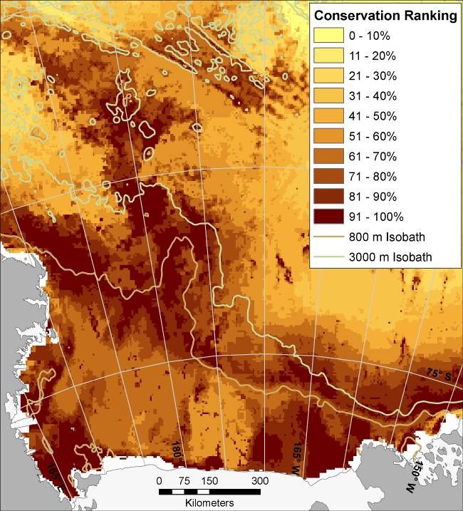
utilization space,” which includes habitat parameters, diet, and patterns of co-existence with
other species (Elton 1927, MacArthur & Levins 1964, Diamond & Case 1986, Wiens et al.
2009). According to classic niche theory, especially where resources are limited, species should
be allocated among habitat types according to their relative capabilities to exploit respective
resources, and fewer species should occupy habitats with more unpredictable attributes (Lack
1954, MacArthur & Levins 1964).
     In the earliest days of ecology, detailed records were kept on the conditions present where a
given species was encountered, including field sketches or photographs and the notes made on
specimen tags. In the context of the disappearance or movement of species in the present time of
rapid environmental change, such information has become increasingly valuable in order to
reconstruct a species’ recent history of habitat use (e.g. Barry et al. 1995, Klanderud & Birks
2003). As the science of ecology has matured, the value of species’ occurrence records has
benefited from the development of modeling techniques for revealing species-habitat
relationships, often from somewhat sparsely collected data (Elith et al. 2006, 2008, Phillips et al.
2006, Wiens et al. 2009). This is especially important for areas where little or no sampling has
been directly carried out. Of course, with more and more ground- (or sea-) truthing, models are
improved and validated.
     Owing to the high costs both in time and resources to sample the ocean, the use of models
and spatial analysis has become particularly important to project occurrence patterns of marine
species, for many of whom data are spatially clumped and otherwise sparse. This ability has, at
least theoretically, increased the relevance of the “systematic conservation planning” that is
involved in identifying portions of the ocean that might deserve special management in the face
of competing pressures from human use of resources and other anthropogenic disturbances
(Margules & Pressey 2000, Ariame et al. 2003, Lombard et al. 2007).
     Fortunately, th he Ross Sea, which is the largest continental shelf ecosystem south of the
Antarctic Polar Front but which comprises just 2% of the Southern Ocean, is one of the better
known stretches of south polar seas due to a long history of investigation (see Ross Sea
Bioregionalization, Part I). Importantly, owing to its relative isolation from human civilization,
and protection of its coastal habitat under the Antarctic Treaty, including several Antarctic
Specially Protected Areas involving marine species, it is the anthropogenically least-affected
stretch of ocean remaining on Earth (Halpern et al. 2008). It still has a full suite of top predators,
including large fish, birds, seals and whales (Ainley 2010), and some of these have been shown
to act together to deplete middle-trophic-level species (smaller fish and krill; Ainley et al. 2006,
Smith et al. in press). This wealth of apex and mesopredators in part must result from the Ross
Sea’s unusually high primary production (estimated to be 28% of the total primary productivity
of the Southern Ocean south of 50°) – implying that there are higher than expected amounts of
phytoplankton available at the base of the so-called trophic pyramid (Arrigo et al. 1998, 2008;
Smith & Comiso 2008) and thus the potential for a very robust food web (Smith et al. in press).
Contributing to this exemplary phytoplankton concentration, as perceived by chlorophyll
measurements, is that phytoplankton grazer standing stocks (e.g., krill) occur in lower than
expected levels, in turn potentially explained by the unusual (in today’s world) prevalence of
their upper-level predators (Table 1; Ainley et al. 2006, Baum & Worm 2009, Smith et al. in
press). For these reasons, and especially its relatively pristine condition, elucidating the patterns
of co-occurrence of this Ross Sea fauna within its relatively small confines may offer ecological
insights not possible elsewhere in the world ocean where most top predators have been severely
depleted for a long time (e.g., Pauly & Maclean 2003), and could help to answer the question of

                                                                                                     2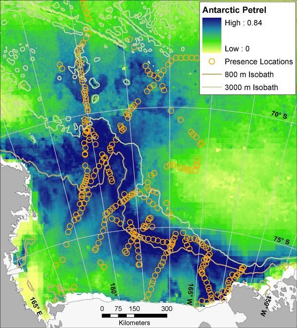
how so many predators can exist there. Here we report results of analyses of niche occupation of
all air-breathing mesopredators in the Ross Sea, considering three important components: 1)
projected distribution and overlap across the surface of the ocean, 2) capacity to utilize differing
amounts of the water column (foraging depth) and 3) diet.
     We knew from the outset (see Ross Sea Bioregionalization, Part I) that certain species would
be too rare or data insufficient to include in spatial modeling, such as Arnoux’s Beaked Whale
Berardius arnouxii (rare) and Colossal Squid Mesonychoteuthis hamiltoni (sparse data, perhaps
rare). It also proved true that data for Antarctic toothfish (Dissostichus mawsoni), coming from
an industrial fishery, were too much affected by a strategy to maximize catch (kilograms) per
unit effort, and have not been summarized by fish size, for use in our modeling of adults (fish
>100 cm TL). It is the adults who, at least by analysis of stable isotopes, occupy the same trophic
level as Weddell Seals (Ainley & Siniff 2009). The lack of information about the distribution of
this mesopredator is unfortunate, given that in most oceans fish are the main predators (Sheffer et
al. 2005), and there is reason to expect an important predatory role in the Ross Sea foodweb as
well (Eastman (1993) characterizes the toothfish as the most important piscine predator in the
Southern Ocean). We also explored including the semi-apex predator, Leopard Seal (Hydrurga
leptonyx), and the apex Killer Whale (Orcinus orca) ecotype A/B (see Pitman and Ensor 2003),
but we had few sightings of the seal in our database (see Ross Sea Bioregionalization, Part I),
owing to their relative rarity and highly localized occurrence pattern during summer (near to
penguin colonies). We made an attempt to model the A/B Killer Whale, which would be the true
apex predator in this system but, as our results show, we failed, likely because of their highly
nomadic life-history. Nevertheless, a broad array of mesopredators was available for analysis and
our results substantially improve understanding of their spatial occurrence patterns in the Ross
Sea, previously only described using heuristic approaches (Ainley et al. 1984, Ainley 1985).

METHODS
1a. Species Distribution Models: Explanatory Variables
We defined the study area as all ocean waters south of 63° S between 165°E and 150°W (Figure
1). Environmental covariates were obtained from various sources (Table 2; see also Ross Sea
Bioregionalization, Part I, for further discussion of these variables, including mapped displays).
    Before inclusion in species distribution models, all covariate data were resampled to 5 km
resolution in ArcMap 9.3.1 using bilinear interpolation or (for sea-ice and chlorophyll) nearest-
neighbor assignment. Although higher resolution bathymetric data are available for parts of the
study area (Davey 2004), we conducted this resampling so that data could be easily matched to
the 5 km bathymetry available for the entire study area (ADD 2000), especially since the
resolution of almost all other source datasets was no better than this (Table 1). Monthly mean
percent sea-ice cover grids were obtained for July to September (winter ice) and December to
January (summer) for ten years, 1998-2008, from the National Snow and Ice Data Center
(Cavalieri et al. 2008) and averaged across all years to obtain one mean grid for each season
(winter and summer). Ice cover data were collected on several of the cruises, but these data were
not available for all locations, and preliminary evaluation of models including these data for
subsamples of locations where they were available did not improve model performance (see
below for description of model evaluation). Slope (rate of change in depth) was derived from the
bathymetry layer (ADD 2000) and was calculated as the maximum change between a given cell
and its 8 neighboring cells, expressed as degrees.

                                                                                                  3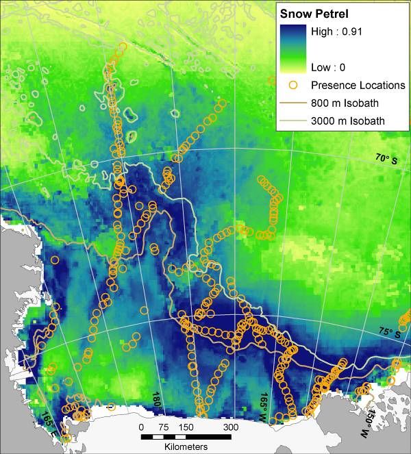
Table 1. Summary of the population size of upper trophic level predators in the Ross Sea, Antarctica, i.e. the waters
overlying the continental shelf and slope. Percentages give, as noted, the portion of the world or Southern Ocean (by
sector) population that occurs within the Ross Sea.
                                                            Percent of
                                           Number           World
Species                                    Individuals      Population      Source
Antarctic Minke Whale                        21,000         6%              Branch 2006, Ainley
Balaenoptera bonaerensis                                                    2010
Ross Sea (Ecotype C) Killer Whale              3350         ~50 %?          Ainley 1985, Ainley et
Orcinus (orca) sp. nov.                                                     al. 2009a, Morin et al.
                                                                            2010
Ecotype-A/B Killer Whale                          70        ?               Ainley 1985, Ainley et
Orcinus orca                                                                al. 2009a
Weddell Seal Leptonychotes                 30,000-          50-72 %         Stirling 1969, Ainley
weddellii                                    50,000         Pacific         1985, Erickson &
                                                            sector          Hanson 1990
Crabeater Seal Lobodon                      204,000         17 %            Ainley 1985, Erickson
carcinophagus                                               Pacific         & Hanson 1990
                                                            sector
Leopard Seal Hydrurga leptonyx                 8,000        12 %            Ainley 1985
                                                            Pacific
                                                            sector
Adélie Penguin Pygoscelis adeliae          3,000,000        38 %            Woehler 1993
Emperor Penguin Aptenodytes                  200,000        26 %            Woehler 1993
forsteri
Antarctic Petrel Thalassoica               5,000,000        30 %            Ainley et al. 1984, van
antarctica                                                                  Franeker et al. 1999
Snow Petrel Pagodroma nivea                1,000,000        ?               Ainley et al. 1984

    We calculated Pearson correlation coefficients for each pair of environmental covariates to
aid in covariate selection and interpretation of model results (Table 3). Prevalence of
Circumpolar Deep Water was relatively highly (negatively) correlated with bathymetry (82%)
and chlorophyll (73%), somewhat complicating interpretation of the relative influence of CDW
versus these variables. However, since our primary goal was to create the best possible
projections of species occurrences rather than to explain why these patterns exist in relation to
covariates, and since they were not completely correlated with one another, we kept them all in
the modeling process, especially given the relative paucity of potential covariates.

                                                                                                                   4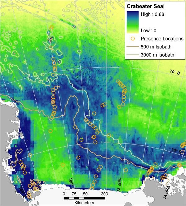
Table 2. Variables used in species distribution models, years of data collection, spatial resolution and source of
original data; see Ross Sea Bioregionalization, Part I, for mapped displays of much of these data.
                                                        Original
                                                        sample
 Data Type                Definition          Years     resolution      Source
 Environmental
 Data
 Bathymetry (BTH)         Depth in                      5km             ADD 2000
                          meters
 Prevalence of            Temperature                   5km             Orsi & Wiederwohl 2009;
 Circumpolar Deep         and salinity                                  http://wocesoatlas.tamu.edu. Also,
 Water (CDW)              defined water                                 Dinniman et al. 2003, M. Dinniman, pers.
                          mass                                          comm.
 Summer Sea Ice           Mean percent        1998 -    25km            Cavalieri et al. 2008.
 (SSI)                    cover (Dec -        2008
                          Jan)
 Winter Sea Ice           Mean percent        1998 -    25km            Cavalieri et al. 2008.
 (WSI); used for          cover (Jul –        2007
 Weddell Seal only        Sep)
 Chlorophyll              Mg x m-3            1997-     12.5km          NASA, J. Comiso, pers. comm.
 (CHL)                    averaged over       2006
                          10 years (Nov
                          – Jan)
 Distance to              Euclidean
 Shelfbreak Front         distance (m) to
 (DSH)                    the 800-m
                          isobath
 Bathymetric              The angle of                  5km
 gradient (SLP)           maximum
                          change
                          between cells
                          in bathymetry
                          grid (degrees)

 Species Occurrence Data

 Minke Whale                                  1976-     5km             D. Thiele, AnSlope cruises (2004); D.
 distribution                                 1983,                     Ainley, RISP and NBP cruises.
                                              1994,
                                              2004
 Killer whale                                 1976-     5km             IWC, R.L. Brownell, Jr, pers.comm.; D.
 distribution                                 2004                      Thiele, AnSlope cruises, D. Ainley, RISP
                                                                        and NBP cruises.
 Seal and seabird                             1976-     5km             D. Ainley, RISP and NBP cruises.
 distributions                                1981,
                                              1994
 Weddell Seal             Positions of        1993-     1km             Pers. comm.: B. Stewart, W. Testa, J.
 distribution             seals with          1995,                     Burns, J. Bengtson, P. Boveng
                          satellite tags      1997-
                                              2000

                                                                                                                     5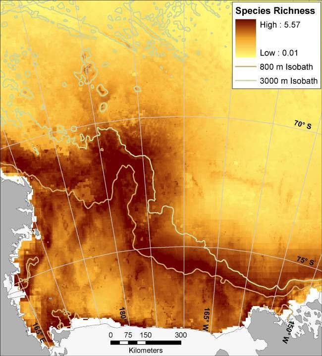
Table 3 Pearson correlation coefficients for each pair of environmental covariates (see Table 2 for explanation of
acronyms).
                 BTH             CDW            SSI                      WSI              CHL               DSH
BTH                -
CDW              -0.82              -
SSI              -0.35            0.23           -
WSI              -0.47            0.34          0.69*                      -
CHL               0.59           -0.73         -0.20                     -0.22              -
DSH              -0.47            0.37         -0.46                     -0.28            -0.35               -
SLP              -0.03            0.24         -0.29                     -0.18            -0.20             0.27
* SSI and WSI were not included in the same models.

1b. Species Distribution Models: Dependent Variables
Sample sizes for all species included in modeling are shown in Table 4.

Minke Whale, Crabeater Seal, and seabirds. Cruises were made aboard ice breakers as listed
below (Fig. 1). Dates encompass periods when the ships were within the study area and are
divided into early summer (15 December to 4 January) and late summer (16 January to 21
February). Before (and since), systematic observations of seabirds this far south were virtually
non-existent for early summer because of the heavy sea ice. Ships and dates of early summer
cruises were: USCGC Northwind, 15 December, 1976 to 4 January, 1977, and 19 December,
1979 to 2 January, 1980; and USCGC Burton Island, 23 December to 29 December, 1977. Late
summer cruises were made on USCGC Burton Island, 16 to 19 and 22 to 26 January, 1977;
USCGC Glacier, 2 to 21 February, 1979; R/V Nathaniel B. Palmer, 12-20 February 1994, and
(AnSlope cruises) 24 February-1 April and 21 October-5 December 2004.
    Counts by (usually) two observers were made from the ice breakers' bridge wings, where eye
level was ~16 m above the sea surface, during hours that the ship traveled at speeds exceeding 6
knots during daylight (more or less continuous). The ships cruised at a maximum 10-12 knots in
open water. In all but AnSlope cruises, in which line transects were made for whales only
(involving >2 observers), continuous surveys were broken into half-hour segments equivalent to
a “transect.” Transects were not made when visibility was
al. 1984), and we have reason to believe that all age classes of marine mammals that utilize the
area were represented, too.

Killer whale. Some data on killer whales were available from the surveys described above, but
most of the presence data used herein came from the International Whaling Commission data
base gathered during the SOWR cruises 1987-2005. On the basis of pod size, as described in
Ross Sea Bioregionalization, Part I, we partitioned sightings into Ross Sea Killer Whale (=
ecotype C; pod size ≥20) and ecotype A and B (combined; pod size ≤10; see Pitman & Ensor
2003).

Table 4. Number of locations where each species was detected and used for creating Maxent species distribution
models.
      Species                                                      No. locations
      Minke Whale                                                       174
      Ross Sea Killer Whale                                              38
      Killer Whale A/B                                                   72
      Crabeater Seal                                                     96
      Weddell Seal                                                     1023
      Emperor Penguin                                                    48
      Adélie Penguin                                                    136
      Antarctic Petrel                                                  329
      Snow Petrel                                                       337
      Light-mantled Sooty Albatross                                      20

Figure 1. Left panel: cruise tracks on which minke whales were surveyed, with bathymetry as base layer (lighter =
shallower). Right panel: tracks on which seabirds and pinnipeds were surveyed (snow petrel sightings used for
example). Right panel also shows typical sea-ice cover for period when most of the cruises were undertaken (mean
Dec-Jan ice concentration from Dec 1997 to Jan 2008 shown – black = no ice, lighter shades of gray = more ice).
See Ross Sea Bioregionalization, Part I for more details.

                                                                                                                    7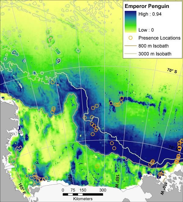
1c. Species Distribution: Maximum Entropy Modeling
We modeled probability of species occurrence using environmental data and species presence
(>0 counted) localities from surveys and sources described in Table 2. Presence data were
aggregated for each 5 km cell in the study area, and locations that fell outside of the extent of any
of the environmental layers were not used. We used a machine learning, “maximum entropy”
modeling method called Maxent (v.3.3.1; Phillips et al 2006, Phillips & Dudík 2008) to estimate
probability of each species’ occurrence in each cell given the modeled relationship between a
given species and the environmental covariates, using Maxent’s logistic output format (Phillips
& Dudík 2008). This is a method that has been used several times recently to achieve goals
similar to ours (Kremen et al. 2008, Stralberg et al. 2009, Carroll et al. 2010). Maximum entropy
modeling can predict species’ distributions from relatively sparse amounts of presence-only
information by estimating the probability distribution that has maximum entropy (most uniform
or spread out across prediction space) while meeting the constraints imposed by the (incomplete)
information available about the actual distribution and avoiding any other assumptions (Jaynes
1957; Phillips et al. 2006; Phillips & Dudík 2008). These constraints require that the mean of
each environmental covariate across the entire prediction space in the model selected by Maxent
be approximately equal to the empirical average of this variable across all sample locations. How
close to equal these means are is a parameter (called “regularization”) that is automatically
optimized by Maxent for each model, but which can be manually specified, with higher values
resulting in lower likelihood of model over-fitting, but also potentially in lower model specificity
(Phillips & Dudík 2008). We ran each model 30 times using a bootstrapping approach using the
full dataset available in a random sort order each time. Thus, the model results presented are the
ensemble means.
    Covariate data in Maxent are allowed to have six types of relationship to the species
occurrence likelihood – linear, quadratic, product (i.e., interaction of two covariates), threshold,
hinge, and category indicator; each type is evaluated with respect to creating the model with the
highest entropy, with the best version retained. Threshold and hinge covariates allow modeling
of an arbitrary response of the species to the covariate from which they are derived (Phillips and
Dudík 2008). Maxent out-performs almost all other existing distribution modeling algorithms
and at least equals the best known methods when compared to known distributions, including
good performance using a limited number of presence locations (Phillips et al. 2006, Elith et al.
2006, Hernandez et al. 2006, Wisz et al. 2008, Phillips & Dudík 2008).
    We produced Receiver Operating Characteristic (ROC) plots (true positives vs. false
positives) based on presence and background (“pseudo-absence”) data (Elith 2002, Phillips et al.
2006). The ROC area under the curve (AUC) values for a randomly selected 25% test portion of
the data in each of 30 model runs was used to evaluate model performance (Table 5). Because
we did not have true absence data, AUC scores represent the probability that a randomly chosen
presence location was assessed to be more likely to have the species present than a randomly
selected pseudo-absence location chosen from the entire study area (Phillips et al. 2006). A
model that does not perform better than random would have an AUC of 0.5, while a perfect
model would have an AUC of 1.0. Models with AUC above 0.75 are considered potentially
useful, 0.80 to 0.90 good, and 0.90 to 1.0 excellent (Swets 1988, Elith 2002). While this method
is not perfect (Lobo et al. 2007), several of the criticisms of AUC do not apply in the context of
this paper (e.g., weighting omission and commission errors equally does not impact our findings,

                                                                                                   8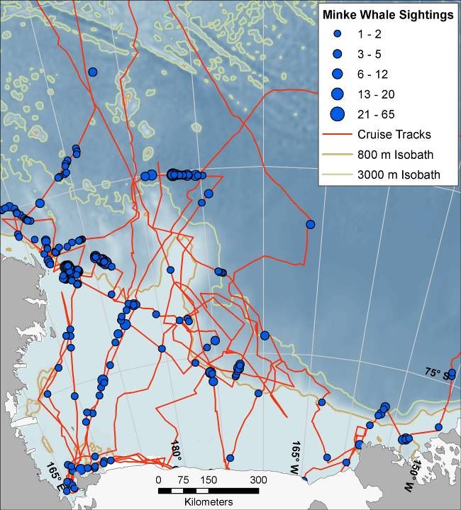
the spatial extent of the models was all the same; Lobo et al. 2007). Model outputs were also
visually inspected and compared to location data and previous expert-based mapping efforts (see
Ross Sea Bioregionalization, Part I). In preliminary validation model runs we investigated
contributions of individual covariates for evidence of model over-fitting and evaluated the effect
of raising the Maxent regularization value above the default settings, with and without
bootstrapping. In all cases best model performance (in terms of test AUC) was achieved by
accepting the default Maxent regularization parameter and bootstrapping. In several cases,
however, inspection of the covariate response curves suggested over-fitting, and increasing
regularization did not penalize AUC substantially (generally 1 - 3%). Thus, for these species we
present bootstrapped results with regularization coefficients set to 2 (i.e., default regularization x
2), and these are the values used in subsequent analyses for Antarctic Petrel, Adélie Penguin,
Snow Petrel, Crabeater Seal, Weddell Seal, and Minke Whale.
    We evaluated another machine learning method for predicting species occurrence, boosted
regression trees, using presence/absence and abundance data (Elith et al. 2008, Leathwick et al.
2008) to validate the maximum entropy results, and to investigate whether multiple interactions
among covariates (up to 5) were influential in predicting species occurrence/absence. We noted
no substantial improvements in results (e.g., in AUC values), and we were not able to use this
method consistently for all species due to the lack or incomplete availability of absence and
abundance data available for some (Weddell Seal, Minke Whale, and both Killer Whale species)
Also, given the limited survey effort for the study area, relative to many other, especially
terrestrial studies (generally only a single visit to any sampling location), we were not confident
that that the absence data available were representative of “true” absences, due to incomplete and
possibly biased survey coverage, which can lead poor modeling results (Mackenzie 2005). For
these reasons we chose to use Maxent for all results reported herein.
    For all species other than Weddell Seal, data represent distribution during December-
February (killer whales to April), and ice and chlorophyll data from that portion of the year was
used in the modeling. During that period, Weddell Seals are concentrated on coastal fast ice,
where even icebreakers rarely pass. Therefore, for Weddell Seals, satellite positions were used,
and mostly from March – October when the seals are free to leave coastal ice cracks and we used
ice data from the middle of that portion of the year (July-September; Fig. 3).

                                                                                                    9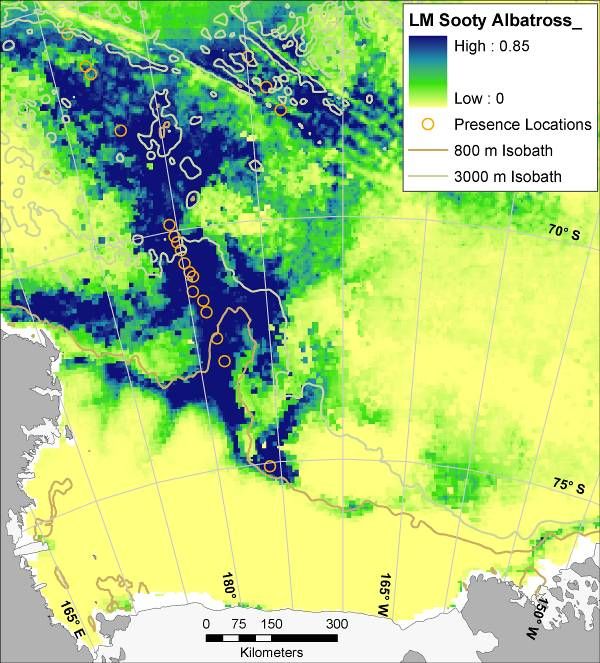
Figure 3. Positions of Weddell Seals during winter as determined by satellite transmitters. Also shown is typical sea
ice cover for the period when positions were determined (mean Jul - Sep ice concentration for 1997 to 2007 shown;
black = no ice, lighter shades of gray = more ice; white is continental ice). These seals were initially tagged outside
the Eastern boundary of the map and subsequently moved into the Ross Sea over the next several months.

                                                                                                                     10
1d. Species Distribution: Comparison of Spatial Overlap, Overall Species Richness, and
identification of relative conservation importance
Using results from the species distribution models, we created an index of the amount of spatial
overlap between every pair of species. To constrain our overlap analysis to those areas that best
represented presence of a species according to the model projections, we applied a threshold to
each model that maximized training sensitivity and specificity (Phillips et al. 2006) and removed
areas that fell below this threshold. We chose this method of conversion because other methods,
such as setting an arbitrary fixed threshold for all species, have been shown to bias results (Liu et
al. 2005). We then multiplied the values of the remaining pixels between each species pair and
calculated the overall mean to get an index of co-occurrence, which equals the mean probability
that both species occurred in any given pixel within their combined ranges. The remaining pixels
were also used to calculate the total area of probable occurrence for each species and of co-
occurrence for each species pair (i.e., the combination of both species’ total area of probable
occurrence) in km2. Weddell Seal was included in this analysis, out of interest, comparing its
winter occurrence patterns with the summer patterns of other species.
To estimate species richness and identify potentially important zones within the study area,
we summed pixel-level probabilities of occurrence (i.e., the original, continuous values produced
by Maxent) across all species.
We used the hierarchical reserve selection software Zonation 2.0 (Moilanen et al. 2005) to
evaluate the relative importance of each pixel in the study area to all species. Zonation
emphasizes conservation priorities from a biodiversity perspective and has been used to evaluate
potential large scale Marine Protected Areas (Leathwick et al. 2008) and terrestrial conservation
priorities (Kremen et al. 2008, Carroll et al. 2010). Zonation offers three advantages over other
reserve design software from our perspective: 1) it allows the creation of a continuous,
hierarchical surface of conservation values across the entire study area; 2) it works from grids
rather than polygons, which simplifies use with other software (especially geographic
information systems) and means that the user is not required to draw any pre-conceived lines on
the map to serve as planning units; and 3) users are not required to set a priori conservation
targets, such as “20% of species X’s range.” We used a simple, unconstrained or “no cost
constraint” approach, where all cells were assumed to have equal potential conservation costs
and prioritization was established simply by evaluating species’ projected distributions and
connectivity, with equal weight given to all species’ “conservation value.” Because we had a
definite list of species for which we wished to rank locations and because we wanted to
emphasize locations with the highest occurrence probabilities we chose to use a core area
definition of marginal loss in the Zonation software, which prioritizes the inclusion of high-
quality locations for all species (Moilanen et al. 2005, Moilanen 2007, Leathwick et al. 2008,
Carroll et al. 2010). For our purposes, the important characteristic of this type of Zonation
analysis is that, assuming comparison of two identical locations with identical projected
occurrence for two different species, the one given higher rank is the one that contains the
species that has lost more of its distribution up to that point in the modeling run. The grid cells
given the lowest ranks are ones that do not contain high occurrence probabilities for any of the
target species, whereas the cells given highest ranks are the ones that contain the highest
probabilities of occurrence for the most species, bearing in mind that species which do not
overlap any others would still need to have some locations retained. The mathematical details
and other methodological information pertaining to core-area Zonation are provided by Moilanen
et al. (2005) and Moilanen (2007).
112. Depth of Foraging
We obtained information on maximum depth of diving, a measure of foraging capability, from
the literature (Fig. 4). Obviously, the ideal would be to investigate all the Ross Sea
mesopredators simultaneously, as seemingly food availability and competitive interactions would
affect diving behavior; indeed, Adélie Penguins forage deeper when in the company of Minke
Whales (Ainley et al. 2006; Ballard et al. unpubl. data). In any case, we could not use mean
depth of foraging in any situation, as this information is not available for all species, i.e., not for
Minke Whale, which was estimated on the basis of body size, killer whale, nor the petrels. For
each species pair, we then determined degree of overlap by dividing the depth of the species
having shallowest dives by that of the one having deeper dives.
Crabeater
Albatross
LM Sooty
Antarctic
Emperor
Penguin
Penguin
Weddell
Adelie
Petrel
Seal
Seal
Whale
Whale
Minke
Petrel
Snow
Killer
0
Maximum Depth Foraging (m)
100
200
300
400
500
600
700
800
Figure 4. Overlap in the maximum diving depths exhibited among top-trophic (air-breathing) predators of the Ross
Sea shelf and slope. Data on diving depths from: Kooyman 1989, Schreer & Kovacs 1997, Baird et al. 2003, Burns
et al. 2004, Ballard et al. unpublished data. Depth for minke whale estimated based on comparable body size to
killer whales (Baird et al. 2003); diving depth generally correlates to body size in vertebrates (see Kooyman 1989).
Instrumented Weddell Seals have been constrained by bottom depth in regard to the maximum depths that they
could attain (thus likely an underestimate?); the much smaller Crabeater Seal, on the other hand, has been
investigated where bottom depth would not constrain deep diving. On the basis of arguments presented in Kooyman
(1989), Weddell Seal should be capable of diving much deeper than has been measured.
3. Diet
We determined an index to the degree of diet overlap among species pairs using data from the
literature on frequency of occurrence of krill (Euphausia superba, E. crystallorophias) and
silverfish (Pleuragramma antarctica) in the diet (Fig 5). These are the two prey types/species
that predominate in this system (summarized in Smith et al. 2007, in press; see also Ross Sea
Bioregionalization, Part I). We could not use other measures, such as diet based on mean mass of
prey nor index of relative importance, because not all species had sufficient detail available (e.g.
minke whale, killer whale). For krill, and then independently for silverfish, we determined the
percent of overlap by dividing the species having the lowest frequency by that having the higher;
we then averaged the two (krill, silverfish comparisons) for each species pair. For a species not
12preying on one of the two diet species (e.g. Weddell Seal: silverfish only) compared to a predator
not preying on the other (e.g. Crabeater Seal: krill only), we considered this 0% overlap rather
than 50% overlap.
100 Silverfish Krill
80
Frequency in Diet
60
40
20
0
Antarctic
Albatross
Weddell
Petrel
Crabeater
Emperor
Whale
LM Sooty
Penguin
Whale C
Snow
Minke
Penguin
Adelie
Petrel
Killer
Seal
Seal
Figure 5. Prevalence of Antarctic silverfish and krill (all species) in the diet of (air breathing) top-predators over the
Ross Sea shelf and slope, thus indexing degree of diet overlap. Data from Ainley et al. 1984, 2003; Burns et al.
1998, Cherel & Kooyman 1998, Green & Burton 1987, Pitman & Ensor 2003, and Ichii et al. 1998. Values shown
for minke whales are a large underestimate for silverfish, as Ichii et al. only presented the proportion of samples in
which silverfish was the dominant prey, not the proportion of samples in which silverfish occurred; values for killer
whales are a guess (the only fish available to them in any quantity would be silverfish and toothfish; see Ainley et al.
2009a).
RESULTS
Model Performance
Model (test data) AUC scores ranged from 0.745 (Killer Whale A/B) to 0.926 (Weddell Seal and
Light-mantled Sooty Albatross) and averaged 0.857 (Table 5). The most influential variable in
species distribution models overall was distance to the shelf break, followed by prevalence of
Circumpolar Deep Water. Distance to shelf break was negatively correlated with probability of
occurrence for all species except Weddell Seal (Appendix). Slope was the least influential
variable overall. Response curves and standard deviations for variable influences for all models
are in the Appendix.
Three patterns of spatial use of the Ross Sea became apparent: 1) Shelf Break: restricted
mostly to the shelf break, which includes outer shelf and the slope (Light-mantled Sooty
Albatross; Fig. 6); 2) Shelf and Slope: full use of both the shelf and the slope (Ross Sea Killer
Whale, Weddell Seal; Fig. 6); and 3) Marginal Ice Zone (MIZ; pack ice surrounding the Ross
Sea post-polynya): combinations in which the slope is the main habitat but western and eastern
portions of the shelf are used as well (Minke Whale, Crabeater Seal, penguins, petrels; Fig. 6).
This last pattern is consistent with correlation to the presence of pack ice, either over the slope or
over the shelf (cf. Karnovsky et al. 2007).
13Table 5. Species distribution model performance (mean AUC ± standard deviation for 30 bootstrapped runs using all
data) and heuristic estimates of percent contribution of each variable to the Maxent model. Bold font indicates most
influential variable in each species’ model; winter sea ice cover used for Weddell Seals (for others: summer sea ice).
Percentage Contribution to distribution model
Distance
Sea Ice Prevalence Shelfbreak Bathy
Common Name AUC ± SD1 Chloro Bathy Cover CDW Front Gradient
Minke Whale 0.923 ± 0.008 14.7 9.4 9.3 13.3 49.5 3.9
Ross Sea Killer 0.934 ± 0.02 8.0 9.0 6.7 57.0 13.2 6.2
Whale
Killer Whale A/B 0.814 ± 0.03 9.2 23.7 16.9 16.8 15.4 18.0
Crabeater Seal 0.871 ± 0.015 5.3 6.4 15.5 19.8 48.8 4.2
Weddell Seal 0.926 ± 0.002 3.7 40.9 7.3 20.0 27.2 0.9
Emperor Penguin 0.928 ± 0.01 4.0 12.3 13.6 8.5 52.5 9.0
Adélie Penguin 0.906 ± 0.009 7.9 13.6 6.2 30.6 39.1 2.6
Antarctic Petrel 0.820 ± 0.008 6.2 3.3 22.7 23.6 41.8 2.4
Snow Petrel 0.852 ± 0.008 12.5 6.3 12.1 18.9 46.9 3.3
Light-mantled 0.962 ± 0.008 27.2 20.0 24.9 14.9 9.4 3.5
Sooty Albatross
Total 98.7 144.9 135.2 223.4 343.8 54.0
1
AUC’s reported in table are for full dataset used in models. AUC’s for bootstrapped test data (random 25% subset
of each of 30 model runs): Minke Whale: 0.896 ± 0.02; Ross Sea Killer Whale: 0.881 ± 0.05; Killer Whale A/B:
0.745 ± 0.07; Crabeater Seal: 0.803 ± 0.03; Weddell Seal: 0.926 ± 0.004; Emperor Penguin: 0.884 ± 0.04; Adélie
penguin: 0.885 ± 0.02; Antarctic Petrel: 0.797 ± 0.02; Snow Petrel: 0.823 ± 0.02; Light-mantled Sooty Albatross:
0.926 ± 0.04.
14Figure 6. Mean (from 30 bootstrapped runs) modeled probability of occurrence for marine predators in the Ross Sea,
Antarctica; results of maximum entropy modeling using Maxent. Presence locations from which models were
created are displayed as orange circles (see Figure 3 for Weddell Seal presence locations, and see Figure 1 for full
survey effort). Map for Weddell Seal is for winter distribution (all others are summer). During summer Weddell
seals are confined mostly to haul outs along the coast, i.e. tide cracks between fast ice and shore. Such habitat was
not adequately sampled by ship-based surveys. LM = ‘Light-mantled’ in the LM Sooty Albatross map.
15Figure 6 (continued)
16Figure 6 (continued)
Analysis of species overlap indicated relatively little overlap in horizontal space. The highest
overlap was between Antarctic and Snow petrels (26%; Table 6), while most species did not
overlap more than 20% (median = 15%) in projected probability of co-occurrence, thus
indicating relatively well-distributed occupation of potential spatial niches. In other words, these
species’ occurrence constituted a sort of mosaic of Ross Sea space. The test AUC score for Killer
Whale A/B was 15% (the median
for summer species co-occurrence) are shown in bold font.
Percent Overlap
Species Area,
Species km2 1 2 3 4 5 6 7 8
1. Minke Whale 441,200 -
2. Ross Sea Killer Whale 247,050 11 -
3. Crabeater Seal 627,750 16 10 -
4. Emperor Penguin 331,625 13 7 18 -
5. Adélie Penguin 548,000 15 9 19 16 -
6. LM Sooty Albatross 271,375 7 4 8 6 4 -
7. Antarctic Petrel 643,475 19 13 21 15 15 12 -
8. Snow Petrel 738,700 17 12 23 17 18 8 26 -
9. Weddell Seal 424,975 15 14 19 17 18 5 18 20
17Species Richness and Conservation Ranking
The species richness analysis integrated the spatial models of all upper trophic level predators.
Even more than the individual models, the species richness model highlighted the importance to
Ross Sea biodiversity of the shelf break region, and other places on the shelf (the troughs
between banks; Fig.7A) where the intrusion of Circumpolar Deep Water was most prevalent, and
also the Ross Island vicinity. See maps of CDW in Ross Sea Bioregionalization, Part I (also
Dinniman et al. 2003, and pers. comm.). While CDW generally was negatively correlated with
species’ probabilities of occurrence (Appendix), this is likely because of its prevalence in the
pelagic portion of our study area, where most species were less likely to occur.
Zonation conservation ranking results also highlighted the importance of most of the Ross
Sea shelf break (outer shelf and slope), Ross Island vicinity, and troughs in the shelf, but also
elevated the importance of the Eastern Ross Sea shelf and pelagic waters overlying areas of
bathymetric complexity (ridges in northern part of study area; Figure 7B).
A. B.
Figure 7. (A) Modeled species richness (sum of individual species’ Maxent-modeled probabilities of occurrence) of
mesopredators of the Ross Sea: Ross Sea Killer Whale (ecotype C), Minke Whale, Crabeater Seal, Weddell Seal,
Emperor Penguin, Adélie Penguin, Antarctic Petrel, Snow Petrel, and Light-mantled Sooty Albatross. (B) Relative
conservation importance for same species; results from Zonation core area analysis with all species given equal
conservation priority (darker colors represent higher conservation ranking).
18Partitioning of Vertical Space and Diet
A review of the literature revealed that among Ross Sea mesopredators a high degree of
partitioning of the shelf and slope habitat exists in the vertical dimension. Species with strong
use of the shelf, and which are present during the winter as well, i.e. Weddell and Crabeater seals
and Emperor Penguin (and adult, therefore neutrally buoyant, Antarctic Toothfish), all are
capable of using the entire water column from the shelf bottom to the surface and, thus,
experience among themselves >70% overlap in foraging depth (Figure 3, Table 7). Only over the
deeper waters of the slope could any vertical spatial partitioning be expressed, other than that
aspect of dive behavior affected by the prey being targeted. Deep diving by the seals and
Emperor Penguin provides access to maximum water volume without needing much horizontal
movement, which would be constrained by the heavy pack ice conditions of winter. The
remaining mesopredators are composed of medium-deep divers (whales), shallow divers (Adélie
Penguin), and surface foragers (petrels, albatross). Complete overlap in foraging depth exists
among the aerial birds and among the whales. Otherwise, there is little overlap in foraging depth
by the majority of species.
Table 7. Percent overlap in maximum diving depth among Ross Sea top mesopredators.
Species 1 2 3 4 5 6 7 8
1. Minke Whale
2. Killer Whale C 1.00
3. Crabeater Seal 0.53 0.53
4. Weddell Seal 0.47 0.47 0.81
5. Emperor Penguin 0.65 0.65 0.80 0.72
6. Adélie Penguin 0.40 0.40 0.21 0.19 0.26
7. LM Sooty Albatross 0.00 0.00 0.00 0.00 0.00 0.01
8. Antarctic Petrel 0.01 0.01 0.01 0.01 0.01 0.04 0.20
9. Snow Petrel 0.00 0.00 0.00 0.00 0.00 0.01 1.00 0.20
Based on a literature review of mesopredator diet, it appears that the deep-diving year-
round/winter inhabitants, Weddell Seal and Emperor Penguin, are mainly piscivorous,
particularly preying on Antarctic silverfish (Fig 5, Table 8). The silverfish, or “herring of the
Antarctic” (DeWitt and Hopkins 1977), is also confined to the shelf, and perhaps its existence is
key to the wintertime presence and deep diving of these predators. As noted above, these
predators, along with adult toothfish, also completely overlap in depth of foraging. The Ross Sea
Killer Whale (ecotype C) to a small degree may be included in this diet pattern. Feeding just on
fish, it likely does not dive as deep and, as far as is known, probably departs the area during
winter (R. Pitman pers. comm.).
Otherwise, the degree of overlap in diet among the remaining species, except for the near-
surface feeding petrels and albatross, is appreciable though less than the above, i.e. ~50%, in
most comparisons. Predators that forage heavily on krill, and tend to not dive deeply, occur
principally over the slope (Minke Whale, Crabeater Seal, albatross). The outer shelf and slope is
where krill biomass is maximum (Ross Sea Bioregionalization, Part I).
19Table 8. Approximate average percent overlap in diet among Ross Sea mesopredators; overlap based on frequency
of occurrence of silverfish in the diet averaged with that of krill in the diet.
Species 1 2 3 4 5 6 7 8
1. Minke Whale
2. Killer Whale C 0.45
3. Crabeater Seal 0.50 0.00
4. Weddell Seal 0.28 0.63 0.00
5. Emperor Penguin 0.58 0.53 0.35 0.42
6. Adélie Penguin 0.80 0.67 0.47 0.47 0.76
7. LM Sooty Albatross 0.50 0.00 1.00 0.00 0.35 0.47
8. Antarctic Petrel 0.85 0.50 0.40 0.37 0.70 0.68 0.40
9. Snow Petrel 0.75 0.30 0.45 0.47 0.82 0.91 0.45 0.74
DISCUSSION
Both the importance of the outer shelf and slope to the Ross Sea mesopredator community and
the mosaic spatial pattern by which these predators used this habitat was noteworthy. To our
knowledge this is the first time that modeling of spatial use and niche overlap among the
majority of mesopredators within an ecosystem — cetaceans, pinnipeds and seabirds —has been
attempted in a marine setting. It has been done for terrestrial habitats, particularly in the context
of the recent “experiments” undertaken when apex predators have been re-introduced, with
resulting cascading effects on the diet and space use of mesopredators, the apex predators having
been absent for decades (McLaren & Peterson 1994, Ripple & Beschta 2004, Prugh et al. 2009).
Competition and niche overlap has also been investigated among numerous, closely related
assemblages of terrestrial vertebrate species, such as birds, lizards, and small mammals
(reviewed in Diamond & Case 1986).
In marine systems, recent food web modeling could be used to assess trophic overlap, if only
indirectly, as for instance the analyses of Österblom et al. (2007) for the Baltic Sea, Watermeyer
et al. (2008a, b) for the Benguela Current, or even Pinkerton et al. (2008) for the Ross Sea.
However, this modeling does not include the spatial and behavioral aspects that also structure
ecosystems, are of great importance to species’ coexistence, and in fact are important to a species
existence in a given region. Aspects of coexistence have been investigated for portions of upper
trophic levels in some marine systems, for instance among predatory fish, seabirds and cetaceans
in the California Current (Ainley et al. 2009b, Ainley & Hyrenbach 2010), studies in which
spatial and temporal use patterns, as well as behavior and diet proved to be important. It was
found, for example, that predatory fish and cetaceans can affect the niche space of seabirds,
sometimes through facilitation and others through competition, a subject which we will return to
below.
The mesopredators of the Ross Sea are dominated by year-round (seals, Emperor Penguin,
possibly the petrels, which forage well in the dark; Ainley et al. 1992) or near year-round species
(Adélie Penguin). Only the albatross and the cetaceans are seasonal visitors, and the cetaceans
are not central place foragers. Therefore, we believe our modeling has identified the “critical
20habitat” (as opposed to commuting habitat) of this fauna. In a mosaic of habitat use, respective
spatial use of the Ross Sea among mesopredators had three patterns common to various groups
of species: most of shelf and slope, mostly slope, and MIZ (which includes waters overlying the
slope). It is not surprising that earlier separate analyses found both the Ross Sea Shelfbreak Front
and the MIZ to be important to these organisms (see Ainley & Jacobs 1981, Karnovsky et al.
2007). Our model of species richness (spatial use of all predators together) and the Zonation
results (showing areas of relative importance to all species) integrated these studies, as well as
the spatial use patterns of the individual mesopredators, and showed that the Ross Sea shelf and
slope, in a spatio-temporal mosaic are a natural history unit at the community scale. Individual
and combined models also showed the consistent importance of the shelf in determining
likelihood of occurrence, with distance to slope (and Shelfbreak Front) being the most influential
covariate we examined (increasing distance from shelf break led to decreasing probability of
occurrence for all species except Weddell Seal). This is further reinforced by a year-round
analysis of Ross Sea use by Adélie Penguins (Ballard et al. 2010; see also Rosss Sea
Bioregionalization, Part I), and a recent comparison of the importance of ocean fronts to
Southern Ocean seabirds, Antarctic-wide: in cases where the Antarctic Shelfbreak Front
coincided with various MIZs, it is the oceanic front rather than the ice front that is the more
important in explaining species occurrence (Ribic et al. 2010). On the other hand, in the Ross
Sea, the MIZ represents a habitat where the microbial community, namely the prevalence of
diatoms, is the basis for a much more complex food web than that originating with Phaeocystis
antarctica, a colonial alga that dominates the central-southern Ross Sea shelf where sea ice is
less persistent (reviewed in Smith et al., in press). Accordingly, many Ross Sea upper trophic
level species appear to avoid the central-southern Ross Sea shelf, where the main predators
appear to be pteropods.
The importance of the outer shelf and slope to Ross Sea predators returns us to the question
raised in the Introduction: how can such large populations of predators, apex- and meso- alike,
exist in the relatively small confines of the Ross Sea? The fact that there are so many Ross Sea
mesopredators seemingly explains the documented trophic cascade in which zooplankton
standing stock is kept low, with lower-than-usual grazing on phytoplankton (summary in Baum
& Worm 2009, Smith et al. in press).
Spatial separation mosaic is part of the mechanism of species coexistence in this system, with
diet segregation playing a minimal part. Diet overlap among mesopredators ranges from medium
to high. Diet overlap is especially high among the petrels and Adélie Penguins, and between the
albatross and Crabeater Seal. The fact that diet overlaps extensively is not surprising given that
just three prey are the main species consumed in this system (two krill species, silverfish). The
relative abundance of these prey (compared to other anthropogenically altered systems), resulting
from the high level of primary productivity, would further facilitate the diet overlap among
mesopredators. Indeed, where diet becomes an important component of niche separation, often it
is expressed mainly when food availability is low (Grant & Grant 1993, Grant 1999, Ainley &
Boekelheide 1990), which is not the case in the Ross Sea. On the other hand, it appears that
differences in depth of foraging are very important to various species’ coexistence, especially for
those species having similar diet, as is the spread of areas where different species concentrate.
To some degree the spread of spatial use may be an artifact of out-of-phase natural history
cycles, which actually would contribute to co-existence at the Ross Sea scale. (1) The penguins
and the Weddell Seal, being central place foragers, are constrained to exist very close to land
during spring and summer (Their confinement was one factor that we propose caused the poor
21performance of the spatial model of the apex predator, Killer Whale B, in that these killer whales
would be keying on several different prey, penguins and seals, and not necessarily habitat). Other
than the extreme western and eastern portions of the Ross Sea, where most penguin colonies and
Weddell Seal haulouts are located, there is much of the outer shelf and slope devoid of them
(other than non-breeding members of their population) during spring-summer, and thus
providing little overlap with other species. In the late summer-autumn the penguins move from
the western Ross Sea to the eastern Ross Sea Shelfbreak region in order to fatten and molt; the
Weddell Seals move out into the Ross Sea beginning late autumn and into the winter, a time
when other species are migrating out of the area (see Ross Sea Bioregionalization, Part I). The
seals tend to occur over deeper areas. (2) Most of the petrels that frequent the Ross Sea slope do
so from the east, apparently closer to (mostly unknown) breeding areas in the mountains of
Marie Byrd Land and Ellsworth Land (Ainley et al. 1984). These petrels forage as they go,
mainly along the shelfbreak, which is close to shore where they begin their flights over the
ocean; thus including waters over which they are merely commuting is not an issue. This eastern
portion of the Ross Sea is the area frequented late in the summer by the penguins during molt,
but coexistence is possible among petrels and penguins owing to a disparate depth of foraging.
(3) Light-mantled Sooty Albatross, although not abundant and therefore somewhat
inconsequential, competitively speaking, are more prevalent in the western Ross Sea slope (and
waters to the north), also possibly being a function of proximity to closest nesting sites (in the
New Zealand subantarctic islands). In fact, their occurrence immediately north of the Shelfbreak
Front, unlike the continent-breeding petrels, may to some extent be due to the detection of
commuting birds. (4) Minke Whales are most abundant in the western slope region, too, an area
in which Blue Whales (Balaenoptera musculus intermedia) were once more abundant; it is likely
that minkes are now more abundant in the Ross Sea as a consequence (Laws 1977, Ainley 2010).
If they need to, Minke Whales can forage deeper than the petrels, albatrosses and Adélie
penguins that co-occur with them, and where Minke Whales are abundant, it is true that penguins
have to adjust their foraging behavior (Ainley et al. 2006).
Competition surely plays a role in spatial use patterns. As noted, we know that when and
where Minke Whales are abundant within the space used by (foraging) breeding penguins, the
whales’ (or whales’ and penguins’ together) foraging causes prey to become less available,
causing expanding foraging area for penguins (and presumably the whales), and deeper diving
for Adélies (Ainley et al. 2006). We expect that this phenomenon occurs along the western Ross
Sea outer shelf and slope as well, which is adjacent to very large (uninvestigated) penguin
colonies in northern Victoria Land, and where Minke Whales are most abundant according to our
model (as well as empirical data; see Ross Sea Bioregionalization, Part I). Indeed, without the
ability to exploit the entire water column, Adélie Penguins are forced by intra- and interspecific
competition to enlarge their foraging areas mostly horizontally as they force the decreased
availability of their prey: large colonies expand foraging areas even more than smaller ones
(Ballance et al. 2009). Emperor Penguins, however, do not show the pattern of seasonal change
in foraging extent (see Ross Sea Bioregionalization, Part I); but if they experience the same sort
of competition that leads to expanded foraging area among Adélies (facilitated by diet
competition with Weddell Seals, and Ross Sea Killer Whales), Emperors hypothetically have a
much better capacity to expand the vertical aspect of foraging than do Adélies. This supposition
in regard to Emperor Penguins needs to be investigated with season-long deployment of time-
depth recorders, as has been done with Adélies (Lescroel et al. 2010). Finally, it is known that
large toothfish disappear from areas where Weddell seals are concentrated. Whether this is due
22to depletion by the predating seals, or movement away by the toothfish owing to competition for
silverfish or harassment by the seals requires more investigation (reviewed in Ainley & Siniff
2009). It is another example of how species interactions may modify spatial use of the Ross Sea,
as indicated in the models generated based on habitat features alone.
We surmise that competition helps to explain some of the other spatial patterns observed. For
instance, why are there no Humpback Whales (Megaptera novaeangliae) in the Ross Sea, but
large numbers immediately to the west (cf. Branch 2009, Ainley 2010)? Is this the result of the
large number of Minke Whales, a known competitor (Friedlaender et al. 2008)? Is it just an
artifact that our model shows relatively few Ross Sea Killer Whales (fish eating) in the
southwestern Ross Sea, where Weddell Seals are probably the most concentrated during summer
of anywhere in Antarctica? These patterns, too, require additional research for a better
understanding of causation.
Limitations of the Study and Final Thoughts
Predicting species probability of occurrences from presence only data is not an ideal approach –
it would be more powerful to have the capability to use true absence information along with
abundance data to create projections of numbers of individuals utilizing each grid cell. As
described in Methods, we did do some comparisons with results from boosted regression trees
for the species for which we had potentially suitable information and did not note any important
differences in patterns of spatial distribution or areas of apparent importance. For the two
penguins and Crabeater Seals, we also have satellite tracking data (displayed in Ross Sea
Bioregionalization, Part I: table 2 and figures 35, 40-43), which show concordance with the
habitat use identified by the models for these species. In other words, the occupation of waters
overlying the shelfbreak front, primarily, and the shelf is obvious. Finally, Maxent is specifically
designed for working with presence-only data, and has been used in similar conservation
prioritization situations previously (Kremen et al. 2008, Carroll et al. 2010). Of course, more
data collection would likely improve matters as well, especially if covariate data were collected
contemporaneously. This is said, however, knowing that the mesopredators in very few areas of
the Southern Ocean have been investigated as well as in the Ross Sea.
Our study benefitted from the wealth of data that have been aggregated over several decades
by researchers working in the study area (see Ross Sea Bioregionalization, Part I). We were
limited, however, in our ability to include environmental covariates collected at the same time as
species’ observations. Many of the datasets were collected prior to the availability of satellites,
and high spatial resolution data are still not available for sea ice or chlorophyll (limited to
12.5km so far, 25km for much of the study period). Although several of the environmental
variables used in our model are temporally dynamic, they do hold distinct spatial patterns over
long time periods, but it would be better to be able to use data collected at the time of the survey.
Future studies will benefit from higher spatio-temporal resolution of covariates, assuming the
food web remains intact long enough for these studies to be undertaken. Even so, our goal was to
project general patterns of current usage at a 5km scale rather than to explore mechanisms
explaining these patterns. Doing the latter would be of great interest, but would require a directed
multi-investigator effort, something which is difficult to achieve in recent years.
The fact that the Ross Sea is still largely intact allows a chance to investigate these sorts of
phenomena and other factors that once structured marine ecosystems elsewhere but which can
now be investigated only indirectly (see, e.g. Österblom et al. 2007, Christensen & Richardson
2008). An intact ecosystem also allows investigation of the apparent large-scale trophic cascade
23You can also read