Context-dependent variability in the predicted daily energetic costs of disturbance for blue whales
←
→
Page content transcription
If your browser does not render page correctly, please read the page content below
Volume 00 • 2021                   10.1093/conphys/coaa137

                                                                                                                              Research Article

Context-dependent variability in the predicted
daily energetic costs of disturbance for blue
whales

                                                                                                                                                             Downloaded from https://academic.oup.com/conphys/article/9/1/coaa137/6102278 by guest on 01 February 2021
Enrico Pirotta1,2, *, Cormac G. Booth3 , David E. Cade4,10 , John Calambokidis5 , Daniel P. Costa6,10 ,
James A. Fahlbusch4,5 , Ari S. Friedlaender7,10 , Jeremy A. Goldbogen4 , John Harwood3,8 , Elliott L. Hazen9 ,
Leslie New1 and Brandon L. Southall7,10

1 Department of Mathematics and Statistics, Washington State University, Vancouver, WA 98686, USA
2 School of Biological, Earth and Environmental Sciences, University College Cork, Cork T23 N73K, Ireland
3 SMRU Consulting, Scottish Oceans Institute, University of St Andrews, St Andrews KY16 8LB, UK
4 Department of Biology, Hopkins Marine Station, Stanford University, Pacific Grove, CA 93950, USA
5 Cascadia Research Collective, Olympia, WA 98501, USA
6 Department of Ecology and Evolutionary Biology, University of California, Santa Cruz, CA 95060, USA
7 Southall Environmental Associates, Inc., Aptos, CA 95003, USA
8 Centre for Research into Ecological and Environmental Modelling, University of St Andrews, St Andrews KY16 9LZ, UK
9 Southwest Fisheries Science Center, Environmental Research Division, National Oceanic and Atmospheric Administration (NOAA), Monterey, CA

93940, USA
10 Institute of Marine Sciences, University of California, Santa Cruz, CA 95064, USA

*Corresponding author: Department of Mathematics and Statistics, Washington State University, 14204 NE Salmon Creek Avenue, Vancouver,
WA 98686, USA. Email: enrico.pirotta@wsu.edu

..........................................................................................................................................................

Assessing the long-term consequences of sub-lethal anthropogenic disturbance on wildlife populations requires integrating
data on fine-scale individual behavior and physiology into spatially and temporally broader, population-level inference. A
typical behavioral response to disturbance is the cessation of foraging, which can be translated into a common metric of
energetic cost. However, this necessitates detailed empirical information on baseline movements, activity budgets, feeding
rates and energy intake, as well as the probability of an individual responding to the disturbance-inducing stressor within
different exposure contexts. Here, we integrated data from blue whales (Balaenoptera musculus) experimentally exposed to
military active sonar signals with fine-scale measurements of baseline behavior over multiple days or weeks obtained from
accelerometry loggers, telemetry tracking and prey sampling. Specifically, we developed daily simulations of movement,
feeding behavior and exposure to localized sonar events of increasing duration and intensity and predicted the effects of
this disturbance source on the daily energy intake of an individual. Activity budgets and movements were highly variable
in space and time and among individuals, resulting in large variability in predicted energetic intake and costs. In half of our
simulations, an individual’s energy intake was unaffected by the simulated source. However, some individuals lost their entire
daily energy intake under brief or weak exposure scenarios. Given this large variation, population-level models will have to
assess the consequences of the entire distribution of energetic costs, rather than only consider single summary statistics. The
shape of the exposure-response functions also strongly influenced predictions, reinforcing the need for contextually explicit
experiments and improved mechanistic understanding of the processes driving behavioral and physiological responses to
disturbance. This study presents a robust approach for integrating different types of empirical information to assess the effects
of disturbance at spatio-temporal and ecological scales that are relevant to management and conservation.

..........................................................................................................................................................
© The Author(s) 2021. Published by Oxford University Press and the Society for Experimental Biology.
This is an Open Access article distributed under the terms of the Creative Commons Attribution License (http://creativecommons.org/licenses/            1
by/4.0/), which permits unrestricted reuse, distribution, and reproduction in any medium, provided the original work is properly cited.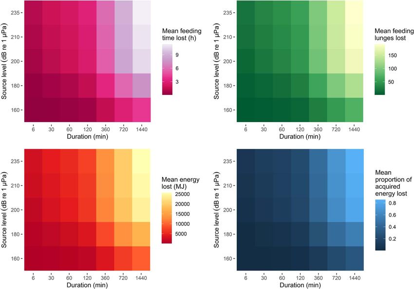
Research Article                                                                                          Conservation Physiology • Volume 00 2021
..........................................................................................................................................................

Key words: Behavioral response studies, data integration, energy budget, marine mammals, navy sonar, population consequences
of disturbance
Editor: Steven Cooke
Received 27 July 2020; Revised 16 December 2020; Accepted 19 December 2020
Cite as: Pirotta E, Booth CG, Cade DE, Calambokidis J, Costa DP, Fahlbusch JA, Friedlaender AS, Goldbogen JA, Harwood J, Hazen EL, New L, Southall
BL (2021) Context-dependent variability in the predicted daily energetic costs of disturbance for blue whales . Conserv Physiol 00(00): coaa137;
doi:10.1093/conphys/coaa137.

..........................................................................................................................................................

                                                                                                                                                             Downloaded from https://academic.oup.com/conphys/article/9/1/coaa137/6102278 by guest on 01 February 2021
Introduction                                                                   changes observed during CEEs to the longer-term effects on
                                                                               survival and reproduction (Houston and McNamara, 2014),
Exposure to human activities can cause changes in the behav-                   thereby facilitating the integration of these responses into
ior and physiology of individual animals (Frid and Dill,                       population-level models.
2002; Beale and Monaghan, 2004). These responses need to
be understood in the context of their long-term effects on                        The quantification of individual energy budgets requires
individual vital rates (such as survival or reproduction) and,                 empirical information on the patterns of behavior animals
ultimately, population dynamics in order to most effectively                   exhibit in the absence of disturbance, such as the time they
inform management actions (Gill et al., 2001; Pirotta et al.,                  allocate to different activities within a day (i.e. their activity
2018a; Ames et al., 2020).                                                     budget), the rates at which they feed and their movements
                                                                               within an area of interest (e.g. Boyd, 1999; Hamel and Côté,
    In the past two decades, concerns over the effects of                      2008; Louzao et al., 2014). Moreover, data on the prey they
military active sonar on marine mammals have stimulated an                     are targeting (such as its patterns of availability, density and
extensive empirical and analytical effort. This has included                   distribution) are essential in order to quantify energy intake,
direct measurements of behavioral responses to sonar by                        the energetic efficiency of foraging and the opportunity to
means of Controlled Exposure Experiments (CEEs) (Southall                      compensate for interrupted feeding (Bowen et al., 2002;
et al., 2016; Harris et al., 2018). Most CEEs use animal-borne                 Grémillet et al., 2004; Goldbogen et al., 2019; Booth, 2020;
electronic loggers and return detailed, high spatio-temporal                   Friedlaender et al., 2020). These data are increasingly avail-
resolution (meters, seconds) information on 3D individual                      able as technology improves our ability to monitor animals’
movements following exposure, e.g. changes in diving behav-                    activity over extended periods and to sample the environment
ior, orientation, vocalizations and location (e.g. Goldbogen et                in which they move (Cade and Benoit-Bird, 2014; Hazen
al., 2013; Friedlaender et al., 2016; Southall et al., 2019a).                 et al., 2015; Calambokidis et al., 2019; Irvine et al., 2019).
Results are typically synthesized into functions describing the                However, behavior, body condition, reproductive state, home
relationship between a given level of exposure (e.g. received                  range and resource availability will vary in space and time and
levels of sonar) and the probability of response (Harris et                    among individuals, resulting in large differences in individual
al., 2018). Parallel analytical developments have formalized                   energy budgets.
a suitable framework to model long-term, population-level
effects of these short-term responses (Pirotta et al., 2018a).                    Changes in behavior resulting from exposure to a
In contrast to CEEs, this framework operates over broader                      disturbance-inducing stressor can also depend on context (e.g.
spatio-temporal scales (e.g. tens of km, days), in part due to                 Ellison et al., 2012). Internal factors (such as behavioral state,
the computational and empirical limitations associated with                    body condition or previous experience), spatial relationships
modelling the entire lifetime of multiple individuals from                     of source and receiver and features of the surrounding
long-lived, wide-ranging species (e.g. Villegas-Amtmann et al.,                environment (e.g. prey quality) can affect the probability
2017; Nabe-Nielsen et al., 2018; Hin et al., 2019; Pirotta et                  of an animal altering its behavior (Ellison et al., 2012;
al., 2019). Therefore, it has proven challenging to integrate                  Houser et al., 2013; Friedlaender et al., 2016; DeRuiter
the detailed empirical information provided by CEEs into a                     et al., 2017; Southall et al., 2019a). Due to the logistical
population-level model.                                                        difficulties and high associated costs of CEEs, data from these
                                                                               experiments often do not support the estimation of exposure-
   Cascading effects from behavior to vital rates are medi-                    response (ER) functions based on separate combinations
ated by an alteration of each individual’s overall health sta-                 of environmental or behavioral conditions (Southall et al.,
tus, for example via disruption of energy budgets (National                    2016).
Academies, 2017; Pirotta et al., 2018a). For cetaceans, this
disruption is mostly driven by an interruption of feeding                         In this study, we integrated diverse data sources to pre-
activity (Noren et al., 2016). Energy can act as a common                      dict the daily energetic costs of simulated disturbance sce-
currency to link the short-term costs of fine-scale behavioral                 narios on individual blue whales (Balaenoptera musculus)

..........................................................................................................................................................
2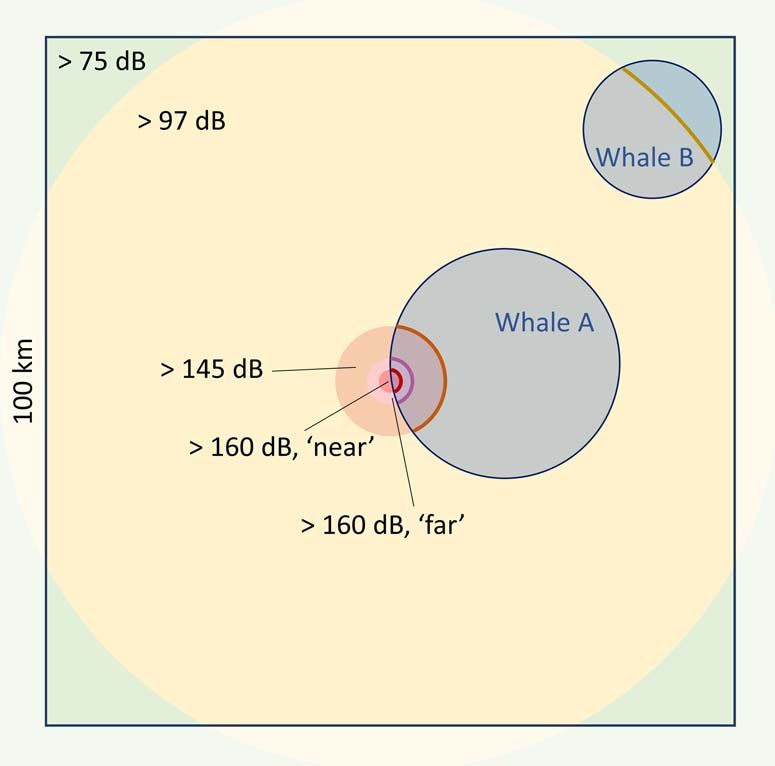
Conservation Physiology • Volume 00 2021                                                                                                Research Article
..........................................................................................................................................................

from the Eastern North-Pacific (ENP) population. Because                       hours based on the proportion of time spent lunging. Blue
its range overlaps with an area used by the US Navy for                        whales in this population engage in two distinct feeding
military training and testing exercises (Calambokidis et al.,                  modes, deep and shallow lunge feeding (Goldbogen et al.,
2009), this population has been the subject of a large behav-                  2015), which involve a different number of lunges per dive
ioral response study, which has generated an extensive CEE                     and trade-off between oxygen access at the surface and food
dataset (Southall et al., 2016, 2019a). Data from experimental                 resources at depth (Hazen et al., 2015). Mean lunge depth
exposures were used to build state- and range-specific dis-                    in each hour was used to determine the predominant feeding
crete ER functions, as well as continuous functions for noise                  mode for that hour (shallow or deep feeding), using a Gaus-
received level (RL) and range from the source. Moreover,                       sian mixture model with two components, fitted with pack-
we derived unprecedented information on baseline behavioral                    age mixtools version 1.1.0 (Benaglia et al., 2009). The first
states, activity budgets, feeding rates, feeding bouts and move-               component had a mean of 33 m (SD = 20 m), corresponding
ments over multiple days or weeks from the activity patterns                   to shallow feeding, while the second component was centered

                                                                                                                                                             Downloaded from https://academic.oup.com/conphys/article/9/1/coaa137/6102278 by guest on 01 February 2021
of individuals instrumented with electronic loggers and that                   on 157 m (SD = 75 m), representing deep feeding. In addition,
were not experimentally exposed to sonar (Szesciorka et al.,                   we extracted the temporal gaps (in hours) between foraging
2016; Calambokidis et al., 2019). Finally, we included mea-                    bouts, that is, the duration of any break (≥1 h) in a sequence
surements of krill densities collected around feeding whales                   of consecutive hours spent in either feeding state (excluding
(Goldbogen et al., 2015, 2019; Hazen et al., 2015) to quantify                 any non-foraging time at the start and at the end of each
expected energy intake in undisturbed conditions. These data                   deployment).
sources were combined to develop daily simulations of whale
movement, feeding behavior and exposure to localized noise                        We used a Markov chain algorithm (package markovchain
sources of increasing duration and intensity. A bioenergetic                   version 0.6.9.7; Spedicato, 2017) to estimate the transition
model (Pirotta et al., 2018b, 2019) was used to estimate indi-                 probabilities between hourly states (deep feeding, shallow
vidual daily net energy intake in disturbed and undisturbed                    feeding and not feeding) and the corresponding stationary
conditions, which provides the common metric needed for the                    distribution (which represents the expected proportion of
integration of experimental results into models of population-                 time spent in each state, i.e. a whale’s daily activity budget).
level consequences. We also assessed the variation in predicted                Daily activity budgets could vary in space and time. Although
costs as a function of the ER curve used, the spatio-temporal                  available data could not support a full exploration of spatio-
subset of activity data that was used to inform whale behavior,                temporal behavioral differences, we wanted to verify whether
krill density distribution and whale size, and identified the                  such variation existed. Therefore, in addition to including the
most important data gaps.                                                      full dataset, we repeated the analysis using only data collected
                                                                               in specific portions of the range or times of the year. Specif-
                                                                               ically, we defined four subsets of the data, corresponding to
Materials and methods                                                          the two spatial and the two temporal subsets containing the
                                                                               highest number of complete individual days (i.e. days with
Multi-day tag data collection and analysis                                     24 hourly records for a given individual). Temporal subsets
                                                                               were defined based on month, while spatial subsets were
Between 2014 and 2019, individual blue whales were                             defined using the latitudinal ranges used to model individual
instrumented with Wildlife Computers TDR10-F tags (n = 21)                     movement in Pirotta et al. (2018b, 2019), to facilitate future
and Acousonde acoustic tags (n = 6), returning GPS location,                   integration of these results in a population-level model. As a
depth and, in most configurations, 3D accelerometry data                       result, the two spatial subsets included data in the latitudinal
for an average of 8 d (range, 1–32 d; Fig. 1a). Details of tag                 ranges 33.8◦ N–34.4◦ N and 37.6◦ N–38.4◦ N, and the two
configurations, deployment and field procedures are provided                   temporal subsets corresponded to data from July and October.
in Supplementary Methods S1 and in Szesciorka et al. (2016)
and Calambokidis et al. (2019). Raw tag data were processed                       We used the Minimum Convex Polygon estimator in pack-
following Cade et al. (2016) to identify feeding events, or                    age adehabitatHR version 0.4.16 (Calenge, 2006) to estimate
lunges. Data were summarized into hourly locations, number                     the area over which an individual ranged in each day (here-
of detected feeding lunges (representing hourly lunge rates)                   after, area covered per day). This estimation was limited to
and mean lunge depth, as detailed in Supplementary Methods                     complete individual days and days where there was some
S1, where we also discuss differences between tags with and                    feeding, i.e. where at least one hour contained feeding lunges.
without 3D accelerometry sensors. The hourly scale was used
to match the resolution of the simulations (see below), and                    CEEs
represented a trade-off between retaining sufficient detail
of an individual’s behavioral variation while keeping the                      Between June and October 2010 to 2014, 42 individual
simulations tractable.                                                         blue whales were tagged with archival electronic loggers in
                                                                               the Southern California Bight and exposed to experimental
   An individual was assumed to be in a feeding state in any                   and operational sound sources. Details of the experimental
hour in which at least one lunge was detected (Goldbogen                       design, field protocols and permits are provided in Southall
et al., 2012). For simplicity, we did not distinguish among                    et al. (2012, 2016, 2019a). The tags recorded fine-scale, 3D

..........................................................................................................................................................
                                                                                                                                                         3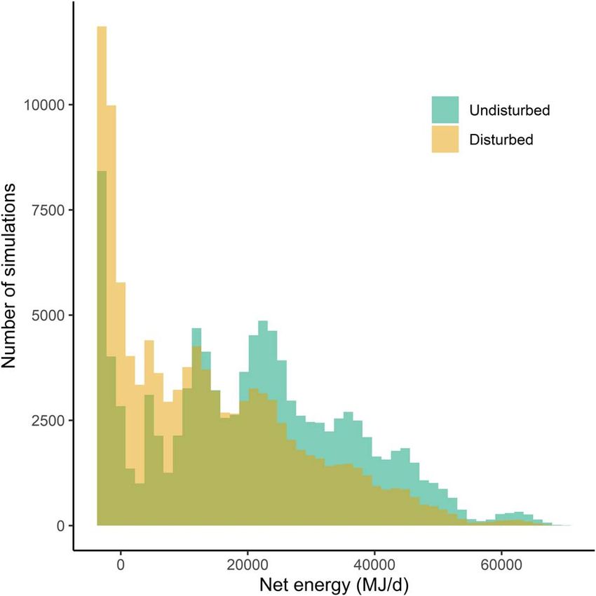
Research Article Conservation Physiology • Volume 00 2021
..........................................................................................................................................................
Downloaded from https://academic.oup.com/conphys/article/9/1/coaa137/6102278 by guest on 01 February 2021
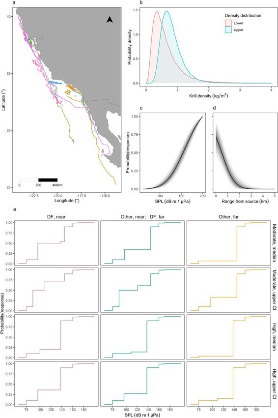
Figure 1: Data used to inform disturbance simulations. (a) Map of multi-day tag data, colored by deployment. (b) Pooled lower and upper krill
density distributions in California. Posterior exposure-response (ER) function for (c) SPL and (d) range from source. The solid line represents the
median, while shaded areas represent 95% credible intervals. (e) Discrete ER functions derived from key assumptions and the survival analysis in
Southall et al. (2019a) for individuals in deep-feeding (DF) or non-deep-feeding (Other) state, either near (within 1 km) or far from (beyond 1 km)
the source (columns). Functions were derived from the median and upper confidence interval (CI) of the moderate and high response severity
curves (rows).
..........................................................................................................................................................
4Conservation Physiology • Volume 00 2021 Research Article
..........................................................................................................................................................
movements, which were analyzed using change-point meth- responding to different RLs (Fig. 1e; Supplementary Methods
ods and a standardized expert-scoring procedure to determine S2).
the occurrence, time and severity of any behavioral change
following exposure, as described in detail in Miller et al. In addition, we developed a continuous ER function
(2012) and Southall et al. (2019a). for received root-mean-square (RMS) sound pressure level
(hereafter, SPL), pooling the data from all individuals
irrespective of behavioral state and range from the source.
We used the expert scoring described in Southall et al.
Development of ER probability functions (2019a) to determine whether an individual was deemed
to have responded with moderate or high response severity
Using the CEE data, we developed three types of ER func- within each experimental exposure, and extracted SPL at
tions (state- and range-specific discrete functions, a contin- the time of the identified behavioral change. If individuals
Downloaded from https://academic.oup.com/conphys/article/9/1/coaa137/6102278 by guest on 01 February 2021
uous function for noise RL and a continuous function for did not respond, we extracted the maximum SPL received
range from the source) and compared the resulting energetic during the experiment. The data were then analyzed using
costs (see below), to investigate the influence of context- the Bayesian approach described in Miller et al. (2014)
dependency and of the metric used to represent the stressor. (Supplementary Methods S2). Finally, we developed a second
continuous function, where range from the noise source was
Southall et al. (2019a) applied recurrent event survival used as the exposure term. We extracted the distance (in
analysis (Harris et al., 2015) to the results of the CEEs to km) between an individual and the source at the time of an
derive blue whale response probability as a function of expo- identified response or, for individuals that did not respond,
sure level in different exposure contexts (differentiated by the minimum distance reached during the experiment,
behavioral state and the range from the source to the whale), and analyzed these data using a modified version of the
for moderate and high response severity scores. Responses approach in Miller et al. (2014) (Supplementary Methods
were strongly context-dependent but sample sizes for certain S2).
contexts were small or absent. First, we therefore derived
relatively coarse ER functions from the results in Southall
et al. (2019a). Distinct conditions were collapsed into three Krill density data
contexts, representing decreasing relative sensitivity: (i) deep-
feeding, near (≤ 1 km from the source); (ii) deep-feeding, far Acoustic backscatter data targeting krill were collected using
(> 1 km from the source), and other states, near; and (iii) other Simrad EK60 or EK80 transceivers at 38 and 120 kHz in
states, far. Being in the most sensitive state (deep feeding) far the Southern California Bight and in Monterey Bay between
from the source was therefore assumed to be comparable to 2011 and 2018, following the field protocols described in
being in another state but close to the source (Supplementary Goldbogen et al. (2019). Hydroacoustic data were analyzed
Methods S2, Fig. S4). according to the predator-scale method described in Cade
et al. (In press) and Cade (2019). The method generates krill
For each context, we related noise exposure level to a density distributions that represent how acoustic cells the
discrete set of response probabilities (1, 10, 50, 90, 99%) size of an average whale engulfment are distributed within
or defined the level at which response probability reached cells the size of an average whale’s horizontal and vertical
an asymptote. Across contexts, 1% response probability was movement during a feeding dive. Two lognormal density
defined as the estimated ambient noise in MFAS band (3– distributions were calculated for each sampling location:
4 kHz) for sea state 3 conditions from Wenz (1962). Ten, one corresponding to the mean distribution, assuming a
50 and 90% response probabilities were derived from the randomly foraging whale (hereafter lower extreme), and
functions in Southall et al. (2019a) where possible. Where the other using the top 50% of data in each dive-sized cell
the corresponding curves reached an asymptote below these (hereafter upper extreme), assuming that a whale chooses
probability values, RLs were determined at respective asymp- where to forage in a patch to maximize efficiency (Cade
totes. Because all functions reached an asymptote below 90% et al., In press; Cade, 2019; Goldbogen et al., 2019). The
probability, the RL corresponding to this probability was means and standard deviations of the distributions at each
determined using estimates of effective quiet from humans, location were then pooled to obtain two distributions of krill
that is, 10 dB below estimates of temporary threshold shift density for the broader California region (lower and upper
(TTS), as proposed by Ward et al. (1976). TTS onset esti- extremes), which are representative of krill biomass available
mates for blue whales (as ‘low-frequency cetaceans’) were to blue whales at a spatial scale matching their foraging
derived from Southall et al. (2019b). Further, these TTS onset behavior (Cade et al., In press). We investigated differences in
estimates were used as the 99% response probability for all krill density in shallow and deep patches (sensu Goldbogen
functions. This procedure returned four step functions (cor- et al., 2015), but did not find any, possibly due to sampling
responding to the median and upper confidence interval of limitations (e.g. the small number of shallow samples, or the
the survival analysis for moderate and high response severity difficulty of characterizing shallow patches using a downward
scores) for each of the three exposure contexts, defining the echosounder). Therefore, the same distributions were used for
probability of an individual in each state and range category all depths.
..........................................................................................................................................................
5Research Article Conservation Physiology • Volume 00 2021
..........................................................................................................................................................
the feeding state in each interval and whether the individual
was within 1 km of the source (‘near’) or further away (‘far’).
Using the continuous ER functions, an individual could
respond every 30 min, i.e. the typical experimental exposure
duration in Southall et al. (2019a). This temporal scale was
thus used to match the temporal scale underlying the devel-
opment of the continuous ER functions. For SPL, we used
bins of 10 dB and calculated the expected range at which
those RL were reached. For range from source, we considered
six distance bins (0–1,..., 4–5, > 5 km) and calculated the
proportion of a day an individual spent in each bin as the
Downloaded from https://academic.oup.com/conphys/article/9/1/coaa137/6102278 by guest on 01 February 2021
proportional overlap between the area covered on that day
and the area in that distance bin. In both cases, response
probabilities associated with each bin were sampled from
a truncated normal distribution defined by the posterior
mean and standard deviation of the estimated ER curve. For
both the discrete and continuous functions, we conservatively
Figure 2: Schematic representation of the simulations using one of assumed that a foraging individual within the area exposed
the discrete exposure-response functions. Shaded blue circles to a given bin of RL or range from source responded with a
provide examples of the areas covered per day by individual whales, probability corresponding to the upper extreme of that bin
resulting in differential overlap with exposed areas. The other shaded (Fig. 1e; Supplementary Methods S3).
regions represent the areas exposed to different ranges of received
levels, where response probability corresponds to the probability at
For each potential response, we randomly sampled an
the upper extreme of that range (warmer colors indicate higher
received levels). Relative ranges are not to scale. empirical gap between foraging bouts from the tag data,
providing a likely inflated (and thus appropriately precau-
tionary given the underlying uncertainty) estimate of the time
required to find a new krill patch after disturbance. All time
intervals corresponding to a behavioral response followed
Simulations by a gap were considered lost. However, if an animal had
responded in a previous interval and was still looking for a
We developed daily simulations of whale behavior to esti- new patch, it did not respond again or lose additional time.
mate the energetic costs of a disturbance-inducing event of For each day, we then tallied the total number of deep-feeding
increasing duration and intensity, occurring at a fixed position and shallow-feeding hours lost, representing the total feeding
within a 100 km × 100 km rectangle (chosen to match the time loss.
spatial resolution of the model used by Pirotta et al. (2018b,
2019); Fig. 2). Given source level (SL), a simple, spherical Using the state-specific hourly lunge rates on that day,
noise propagation model was used to determine the ranges at we computed the total number of lunges lost. For each lost
which RLs of interest were reached (Au and Hastings, 2008). lunge, we drew a value of krill density from the pooled
For each replicate, we sampled a random day from the activity lognormal krill density distribution. Given the length of the
data and calculated the proportional overlap between the area simulated individual (affecting buccal size, as per Pirotta et al.,
covered on that day and the area between two defined RLs 2018b, 2019), krill energy density in the California Cur-
of interest, taken to represent the proportion of a day an rent (Chenoweth, 2018) and assimilation efficiency (Lockyer,
individual was exposed to RLs in that range. 1981), lost lunges were translated into total (gross) energy
For the discrete ER functions, an individual could respond lost on a day, representing the daily energetic cost of that
every 6 minutes, matching the assumptions underpinning disturbance scenario.
their derivation (Supplementary Methods S2). The probabil- We estimated the theoretical gross energy acquired on that
ity of responding at each interval was independent of any day without disturbance, given the bioenergetics equations in
previous exposure or response to sonar. Six-minute intervals Pirotta et al. (2018b, 2019) (Supplementary Methods S3). We
over a day were thus randomly assigned to portions of the divided the total energy loss by the gross energy acquired in
covered area exposed to different RL ranges, based on the undisturbed conditions and obtained the proportional loss in
proportional overlaps, and a behavioral state, based on the energy acquired. This metric could vary between 0 and 1 and
activity budget on the sampled day. Given the time and summarized the proportion of energy acquisition that was lost
duration of the simulated source, we determined if each following disturbance.
interval was exposed and the corresponding range of RL
experienced. Response probability was then determined from The bioenergetics equations in Pirotta et al. (2018b, 2019)
an ER function. Different functions were used depending on were also used to estimate daily energy expenditure, given
..........................................................................................................................................................
6Conservation Physiology • Volume 00 2021 Research Article
..........................................................................................................................................................
the activity budget on each day (Supplementary Methods most data were collected between July and October, with
S3). Net energy intake was then computed as acquired minus animals concentrating in the Southern California Bight and
expended energy for undisturbed and disturbed conditions, in waters off San Francisco and Monterey. The area covered
adjusting energy expenditure following disturbance in light of by individuals over the course of a day (with some foraging)
the altered activity budget. Whenever simulated krill densities varied between 12 and 1647 km2 (mean = 294 km2 ; standard
resulted in foraging costs exceeding energy acquired, we set deviation (SD) = 343 km2 ). The stationary distribution of the
the net intake from foraging to 0; however, the daily net Markov chain suggested individuals spent a variable amount
intake could still be negative if maintenance costs exceeded of time in different behavioral states. Different stationary
foraging gains. The daily costs of reproduction that females distributions were also obtained when the algorithm was run
could potentially incur were calculated for an individual in the on subsets of the data collected in the two most represented
middle of pregnancy (for gestation), or assuming an individual locations and months (Table 1). In contrast, state-specific
delivered the maximum daily amount of milk to the calf (for lunge rates did not vary (Table 1; Supplementary Methods
Downloaded from https://academic.oup.com/conphys/article/9/1/coaa137/6102278 by guest on 01 February 2021
lactation) (Pirotta et al., 2018b). S3, Fig. S5). The temporal gaps between bouts of consecutive
hours with feeding activity ranged between 1 and 226 h
Simulations were repeated for: 1) five SL (235 dB re 1 μPa, (mean = 10 h; SD = 20 h).
i.e. the nominal intensity of 53C sonar; 210 dB re 1 μPa,
i.e. the highest SL achieved during CEEs, comparable to the The lower and upper pooled krill density lognormal dis-
intensity of other Navy MFAS systems, including helicopter- tributions taken to represent the broader California ecosys-
dipping (AN/AQS-22) sonar; 200, 180 and 160 dB re 1 μPa, tem had geometric means 0.513 kg/m3 and 0.757 kg/m3 ,
covering the full range of transmitted source levels associated and geometric SDs 1.917 kg/m3 and 1.468 kg/m3 , respec-
with the wide variety of military activities occurring in the tively (Fig. 1b). The four discrete (median and upper confi-
study area); 2) seven durations of the disturbance-inducing dence interval of the survival analysis for moderate and high
event (6 min, i.e. the average duration of 10 sonar pings at response severity) and two continuous (for SPL and range
maximum level; 30 min, i.e. the average CEE duration; 60, from source) ER functions are represented in Fig. 1c-e. Gibbs
120, 360, 720 and 1440 min); 3) three source positions (at Variable Selection excluded the effects of previous exposure
the center, in a corner or at the center of one side of the and source type on response probability in the latter two
100 km x 100 km rectangle); 4) three whale lengths (22, 25 functions.
and 27 m); 5) two krill density distributions (corresponding
to the lower and upper extremes for the pooled distribution); Given the empirical activity budgets and lunge rates, a
6) six ER functions (four discrete and two continuous). Each body length of 22 m and the lower pooled krill density dis-
scenario resulting from the combination of these conditions tribution, an individual was predicted to acquire 27 663 MJ/d
was replicated 1000 times. Simulations were also repeated (range: 0–82 593 MJ/d) and expend 6592 MJ/d (range: 2555–
using only subsets of the multi-day tag data, corresponding 10 628 MJ/d), on average. When we simulated a disturbance-
to the two locations and the two months encompassing inducing source, the mean feeding time, number of lunges,
most data. For simplicity, simulation results are presented gross energy and proportion of acquired energy that were lost
for a 22-m-long individual (the average asymptotic length of as a result of exposure and any associated behavioral changes
ENP blue whales; Gilpatrick and Perryman, 2008), feeding all progressively increased for increasing intensity (SL) and
on krill densities drawn from the lower pooled distribution duration of the source (Fig. 3). However, even in scenarios
and assuming a discrete ER function corresponding to the involving a weak or brief source, the distribution of these
median result of the survival analysis for moderate response variables had long tails (Fig. 4). In 51% of simulations under
severity scores. Results from the other simulated scenarios are reference conditions, there was no change in the net energy
discussed in comparison to these reference conditions. intake for the day, either because individuals did not overlap
with the source in space or time, or were exposed but did not
Simulations were coded in R version 3.6.2 (R Core Team, respond. In contrast, in 49% of simulations the net energy
2019). The data and code to run these analyses are available intake decreased and in 11% of all simulations it went from
via the Open Science Framework (https://osf.io/q5nbf/?view_ positive to negative (Fig. 5). Gestation costs could increase
only=f7bda77903594328a9ff30cc26b62b78). A list of all abbre- energy expended per day by an average of 7% (range: 4–
viations is reported in Supplementary Methods S4. 15%), while lactation costs represented a mean increase of
77% (range: 41–166%).
Mean gross energy loss was higher for larger individuals
Results and when krill density was sampled from the upper pooled
distribution. Because undisturbed energy acquisition was also
After processing, the multi-day tags provided 5281 hourly higher in these cases, the proportion of daily acquisition that
records of activity and 134 complete days during which the was lost was not affected by these variables (Supplementary
animals engaged in some foraging activity (Fig. 1a). Deploy- Methods S3, Fig. S6). With equal SL and duration, a source
ments spanned from May to November, from Baja California positioned at the center of the location had a greater chance
Peninsula (Mexico) to northern California (25◦ N–40◦ N), but of overlapping with the area covered by an individual within
..........................................................................................................................................................
7Research Article Conservation Physiology • Volume 00 2021
..........................................................................................................................................................
Table 1: Daily activity budget across data subsets
Data subset % time % time % time Mean hours Mean hours Median Median
not deep shallow deep feeding shallow feeding lunge rate lunge rate
feeding feeding feeding [range] [range] deep shallow
feeding feeding
(SD); (SD);
lunges/h lunges/h
Overall dataset 61 29 10 9 [0–17] 3 [0–18] 19 (8) 15 (10)
Latitude range 42 50 8 13 [0–17] 2 [0–11]
33.8◦ N–34.4◦ N
Downloaded from https://academic.oup.com/conphys/article/9/1/coaa137/6102278 by guest on 01 February 2021
Latitude range 46 29 25 7 [0–15] 6 [0–18]
37.6◦ N–38.4◦ N
July 45 48 7 12 [0–17] 2 [0–9]
October 65 32 3 9 [0–15] 1 [0–4]
Figure 3: Predicted effects of disturbance for increasing source intensity and duration, under reference conditions (that is, assuming the
discrete exposure-response function for median values under moderate response severity, the lower krill density distribution and a 22-m-long
individual).
a day, increasing overall exposure (Supplementary Methods time in deep-feeding state and covered smaller areas per day,
S3, Fig. S7). leading to a mean 27% increase in time loss, which, in turn,
led to a mean 45% increase in energy loss, compared to pre-
Using activity data from specific locations affected predic- dictions from the entire dataset. Differences were less marked
tions: in latitude range 33.8◦ N–34.4◦ N, animals spent more in latitude range 37.6◦ N–38.4◦ N due to a combination of
..........................................................................................................................................................
8Conservation Physiology • Volume 00 2021 Research Article
..........................................................................................................................................................
Downloaded from https://academic.oup.com/conphys/article/9/1/coaa137/6102278 by guest on 01 February 2021
Figure 4: Boxplots of the predicted proportion of acquired energy Figure 5: Daily net energy intake (energy acquired-energy
lost due to disturbance, for increasing source intensity (rows) and expended) in undisturbed and disturbed conditions, assuming the
duration. The plot shows the long tails of the corresponding discrete exposure-response function for median values under
distributions. moderate response severity, the lower krill density distribution and a
22-m long individual. Net energy intake was negative when
maintenance costs exceeded the net energy acquired through
feeding. The third color on the graph represents the overlap between
more time not feeding or in shallow-feeding state and larger the histograms.
areas covered per day, resulting in a mean 7% higher time loss
and 5% higher energy loss. Similarly, predictions using only
activity data from July, when individuals engaged in more
deep feeding, indicated a 21% higher time loss and a 29% Discussion
higher energy loss, on average. In contrast, using data from We have demonstrated that diverse data sources obtained
October, when feeding was reduced, led to a mean 19% lower on different spatial and temporal scales, including high-
time loss and a 27% lower energy loss. resolution experimental exposures to disturbance-inducing
Under reference conditions, predicted effects varied stressors, activity monitoring over multiple days or weeks,
depending on what discrete ER function was used. Using the telemetry tracking and prey sampling, can be effectively
function derived from the upper confidence interval of the integrated with a bioenergetic model to predict the effects
survival analysis for moderate response severity caused a 9% of disturbance on an individual’s daily net energy intake. We
higher time and energy loss, compared to using the median. showed that these effects were heterogeneous and depended
Predicted mean effects were 10% lower when median values on the context of exposure. Our approach can be used to
from the curve for high response severity were used, whereas inform population-level inference, thus bridging the gap
they were 1% higher when using the upper confidence between fine-scale, experimental studies and the assessment
interval of the high curve. of the long-term consequences of disturbance.
Predictions differed more substantially when the two con- Daily energetic costs of disturbance: large
tinuous ER functions were used to assess the probability of a
behavioral response. Using the continuous function for SPL,
variability and context-dependency
mean time and energy loss was 63% lower than predicted We found that the daily energetic costs of disturbance on
using the discrete ER function under reference conditions individual blue whales were highly variable. Source intensity
(Supplementary Methods S3, Fig. S8). Because the probability and duration were obvious drivers of such variation, but
of responding at a given range from the source declined to the distribution of predicted costs had long tails, indicating
0 within ∼ 5 km (i.e. resulting in a much smaller impacted that consequences could be dramatic across scenarios: some
area, irrespective of source level), mean effects using this ER simulated individuals, on some days, lost all daily energy
function were 98% lower than predicted using the discrete acquisition, even under brief (e.g. 6–30 min) or weak (e.g.
ER function. 160–180 dB re 1 μPa source level) disturbance events (Fig. 4).
..........................................................................................................................................................
9Research Article Conservation Physiology • Volume 00 2021
..........................................................................................................................................................
In approximately 50% of simulations, net energy intake nistic understanding of whale hearing processes to remedy
decreased and in 11% of simulations it became negative, the paucity of empirical data, they allowed these contextual
indicating an individual would not be able to cover energy variables to be explicitly incorporated in the simulation of
expenditure with the energy acquired on that day. In contrast, responses (Goldbogen et al., 2013; DeRuiter et al., 2017;
in the other 50% of simulations, no change in daily net Southall et al., 2019a). These functions were explicitly pre-
energy intake was predicted, because feeding whales either cautionary; for example, we assumed that animals exposed
were not exposed to the source or did not respond. The to a range of RL responded with a probability corresponding
variability in predicted costs for animals that were disturbed to the higher extreme of the range (thus inflating the effects
resulted from the large behavioral variation recorded in the of disturbance). Nonetheless, predicted costs were notably
tag data, i.e. the differences in activity budget, lunging rates higher compared to the continuous functions. The continuous
and ranging pattern among individuals and days. Observed function for SPL predicted a higher response probability
behavioral patterns, in turn, likely reflected differences in the for intermediate noise levels, but lower probabilities around
Downloaded from https://academic.oup.com/conphys/article/9/1/coaa137/6102278 by guest on 01 February 2021
prey patches targeted by tagged animals (Goldbogen et al., 160–170 dB re 1 μPa; in the discrete functions, these noise
2015; Hazen et al., 2015). Similarly, large variability also levels were assumed to cause a response in most individuals,
emerged when activity data were restricted to a specific based on considerations for levels near or exceeding those
location or month: more intense feeding activity, concentrated required to induce TTS. RLs above 170 dB re 1 μPa are rarely
in smaller areas, as observed in southern California and in achieved in CEEs, due to permit limitations on exposure levels
summer, resulted in considerably higher predicted costs (up to and difficulties in coordinating sources with mobile target
45% greater energy loss) (Pirotta et al., 2018b, 2019). Repro- animals. Thus, this discrepancy remains unresolved. Gener-
ductive costs, especially during the lactation phase (ranging ally, while recent efforts have engaged operational sources,
approximately between December and July for this popula- many CEEs will continue to rely on weaker signals compared
tion), would exacerbate the effect of disturbance on the daily to real sonar sources, with potential implications for the
energy intake (Gittleman and Thompson, 1988). characterisation of cetacean responses, but studies based on
opportunistic exposures to real Navy activities could be useful
Across taxa, including in pinnipeds (Boyd, 1999; Williams (Joyce et al., 2020). The continuous function for distance,
et al., 2007; Dalton et al., 2015; Russell et al., 2015), other on the other hand, predicted a relatively small footprint of
mammals (Hamel and Côté, 2008; Studd et al., 2020) and each disturbance event because there were few experimental
birds (Vézina et al., 2006; Louzao et al., 2014) the time exposures beyond 5 km. The lower SL used in the CEEs and
allocated to foraging and the resulting activity and energy the small number of distant exposures thus impose caution
budgets, is known to be affected by resource availability, on the interpretation of this function.
seasonality, body condition and reproductive state. In parallel,
movement behavior and home range size also vary within Krill density distribution and whale body size affected
and among populations as a function of resource abundance gross energetic loss, but had little influence on the propor-
and season, for example in ungulates (Morellet et al., 2013). tional costs at a daily scale, which were mostly driven by
The large variability in daily behavioral patterns of baleen behavioral variability. However, as noted above, observed
whales could emerge from their foraging strategy, whereby behavioral patterns depend on the characteristics of the prey
the high costs associated with lunge feeding must be balanced patches on which tagged whales were feeding (Goldbogen
with large intake from dense, but patchily distributed prey et al., 2015; Hazen et al., 2015); therefore, prey availability
(Goldbogen et al., 2019). and abundance likely played an indirect role. Moreover, patch
The marked differences among the predicted effects of characteristics are known to vary with depth, with resulting
disturbance on individual blue whales underline the impor- consequences for whale feeding strategies (Goldbogen et al.,
tance of a spatially and temporally explicit evaluation of 2015; Hazen et al., 2015). Unfortunately, we were unable
these effects. Marine spatial planning can be used to minimize to explore the effects of this variability on the predicted
the overlap of disturbance-inducing activities with key areas costs because of sampling limitations, but future data col-
or times for foraging (Foley et al., 2010). More generally, lection should address this critical knowledge gap (Table 2).
our results reinforce the idea that context modulates the Krill density and whale size can also change the probability
predicted costs of disturbance (Gill et al., 2001; Tablado of animals responding to the source (Friedlaender et al.,
and Jenni, 2017). Further data collection is therefore advised 2016; Tablado and Jenni, 2017). More broadly, for long-
to fully characterize movement, foraging patterns and prey lived species with large energy storage and fasting abilities,
availability and density across the population’s range, partic- like the blue whale, it is the energy budget at a longer time
ularly around the under-sampled geographical extremes and scale that ultimately affects survival and reproduction (Pirotta
in winter (Table 2). et al., 2019). In this sense, the variability of krill density at
broader spatio-temporal scales, the number of days without
The influence of exposure context on response probability any feeding and the energy storage capacity of an individual
(e.g. Ellison et al., 2012) was directly addressed here in the whale are critical in determining compensation after distur-
derivation of state- and range-dependent ER functions: while bance, the ability to maintain a positive energy intake over
these functions relied on several assumptions and a mecha- longer periods and the accumulation of sufficient reserves
..........................................................................................................................................................
10Conservation Physiology • Volume 00 2021 Research Article
..........................................................................................................................................................
Table 2: Knowledge gaps and associated data requirements
Knowledge gap Data requirements Study component highlighting the gap
Variation in whale behavior Activity budgets, feeding rates and daily ranging Table 1; Fig. 4
patterns across latitudes and seasons
Variation in prey Prey density measurements in different latitudes, Supplementary Methods S3, Fig. S6; prey density
seasons, and depth strata; prey length and energy content affect an individual’s long-term
distributions; prey energy density energy budget and ability to compensate for
predicted daily energy loss; depth-dependent
densities would change predicted costs of
disturbance when shallow and deep feeding
Downloaded from https://academic.oup.com/conphys/article/9/1/coaa137/6102278 by guest on 01 February 2021
Whale sensory ecology Identification of cues used to locate patches and Simulated responses require information on how
assess their quality quickly and efficiently an individual can resume
foraging after disturbance
Context-dependency in More CEEs for combinations of contextual variables Figs 1, 3; Supplementary Methods S3, Fig. S8
probability of response (e.g. exposures at larger distances and lower
received levels, targeting animals in different states
or feeding on different prey densities)
Realistic exposure scenarios Noise propagation modelling and characterization Fig. 3; source intensity and noise propagation
of disturbance-inducing sources determine an individual’s exposure rate and level
Pathways for adverse effects Measurement of physiological responses to Simulations only included behavioral responses;
disturbance (e.g. stress hormones) the effects of prolonged exposure were only
additive
during the feeding season (Table 2). For example, long-term the large individual, temporal and spatial variability in the
consequences will depend on whether disturbance occurs in predicted energetic costs of disturbance, our results underline
a year where resource availability is favorable or unfavorable that modelling population consequences will require sampling
across the population’s range and on whether an individual is from the distribution of costs, rather than using mean predic-
in good or bad nutritional status when it arrives on the feeding tions. Ignoring this heterogeneity would be misleading, since
grounds (Hin et al., 2019; Pirotta et al., 2019). few individuals incur average costs and some may incur much
higher ones (Biggs et al., 2009).
Data integration and the population
consequences of disturbance Some simplifications to the simulation approach were
required in order to integrate data collected at different
Understanding the long-term consequences of behavioral dis- scales and resolutions. For example, our simple propagation
ruption is challenging, because extensive knowledge of base- model does not capture the effects of specific bathymetry
line behavior and of the characteristics of the environment is and oceanography on noise propagation (Au and Hastings,
required (Pirotta et al., 2018a). In this study, the integration of 2008). Ideally, we would have used information on the
multiple data sources allowed translating observed behavioral
realized footprints of real sonar sources in realistic training
changes into a potential loss of foraging time and associated
operations (Table 2), but such data are not generally
energy, which will provide a common metric to evaluate
available due to security restrictions. Other simplifying
the implications of these short-term responses for individ-
choices were made with regard to individual movements:
ual fitness using models for the population consequences of
disturbance. This reinforces the results of previous work on a realistic movement model derived from telemetry data
other marine mammal (Noren et al., 2016; Farmer et al., could be used instead (Donovan et al., 2017), but fast
2018; Guilpin et al., 2020), mammal (Bradshaw et al., 1998; computation will remain an important feature for real-
Houston et al., 2012) and bird species (West et al., 2002; world applications of any simulation exercise. Moreover,
Masden et al., 2010). Importantly, we were able to partially we used the intervals between foraging bouts to represent
reconcile the mismatch between the scale of data collection the time to find a new patch, similarly to Boyd (1996):
(detailed individual movement and diving behavior, collected in undisturbed conditions, these gaps in feeding activity
in specific locations and times, at extremely high resolu- probably arise from patch depletion or changes in the
tion) and the scale of a corresponding model (Pirotta et al., oceanographic processes supporting krill aggregations (Cade
2019) for population-level effects (dealing with the popu- et al., In press; Santora et al., 2017). However, blue whales
lation, modelled across the entire year and range, at daily appear unlikely to completely leave a foraging area when
temporal resolution and in large spatial units), thereby con- disturbed, often returning to foraging rapidly following
densing the data into a compatible input for the model. Given the abatement of disturbance (Southall et al., 2019a).
..........................................................................................................................................................
11Research Article Conservation Physiology • Volume 00 2021
..........................................................................................................................................................
A better empirical characterization of the cues used to Acknowledgements
locate foraging patches, the distribution of patches in
the environment and the factors affecting the severity of We thank Len Thomas, Catriona Harris and Phil Bouchet for
behavioral responses is therefore needed to inform this advice on the Bayesian analysis. We thank KC Hambleton and
component of the simulations (Table 2). In general, we have Antonia Leeman for their contribution to the lunge detection
followed the precautionary principle when addressing these analysis. Thanks to Emer Rogan and University College Cork
limitations, which has likely led to overestimating the effects for providing desk space to EP. We thank Matt Savoca and
of disturbance. two anonymous reviewers for their useful and constructive
comments on the paper. All research activities for this study
The use of discrete, state- and range-specific ER func- were authorized and conducted under US National Marine
tions relied on several assumptions. Future CEEs should be Fisheries Service permits 14534, 19116, 16111 and 21678.
designed to quantitatively assess the influence of these, and
Downloaded from https://academic.oup.com/conphys/article/9/1/coaa137/6102278 by guest on 01 February 2021
other, contextual factors (Table 2), given the strong influence
they had on our results (Harris et al., 2018). For example,
it will be important to run experiments involving multiple
Funding
exposures and at larger ranges from the source (>5 km). This study was supported by the Office of Naval Research
However, the sample size required to ensure sufficient power (ONR) [grant number N00014–19-1-2464: “BRS4PCoD:
to test complex combinations of conditions and the asso- Integrating the results of Behavioral Response Studies into
ciated high costs of these operations are limiting factors models of the Population Consequences of Disturbance”].
(National Academies, 2017; Harris et al., 2018). An indi- J.A.G., D.E.C. and J.A.F. were supported by the National
vidual’s ability or willingness to change its behavior may Science Foundation (Division of Integrative Organismal
also depend on when exposure occurs within the dive cycle Systems) [grant number 1656691], ONR Young Investigator
and any associated physiological constraint. Importantly, the Program [grant number N000141612477], ONR Defense
probability of responding to a repeated or prolonged dis- University Research Instrumentation Program [grant number
turbance source could change over time, as a result of sen- N000141612546] and Stanford University’s Terman and
sitization or habituation. This would be more accurately Bass Fellowships. The SOCAL-BRS project was supported
represented by an ER function for the aggregate exposure by the US Navy’s Chief of Naval Operations Environmental
to noise (National Academies, 2017). Similarly, some empir- Readiness Division, the US Navy’s Living Marine Resources
ical evidence suggests that animals may be responding to Program and the Marine Mammal Program of the Office of
the total noise energy they receive, rather than the ampli- Naval Research. Cascadia tag deployments were supported by
tude of any one stimulus (Isojunno et al., 2020). Uncer- different divisions of the National Oceanic and Atmospheric
tainty around source characteristics and propagation, and Association including the National Marine Sanctuary
the spatio-temporal scale of animal movements imposed by Program, NMFS-Fisheries and the Section 6 program through
the model, made it unfeasible to use sound energy in this the Washington Department of Fish and Wildlife.
study. Finally, we have focused on behavioral responses, but
increases in stress levels and other physiological effects of
disturbance could also affect an individual’s health status
on the long-term (National Academies, 2017; Pirotta et al., Author Contributions
2018a). E.P., B.L.S., J.H., C.B., J.C., L.N. and D.P.C. conceived
the study; E.P. developed the simulation analysis; D.E.C.,
In conclusion, by building on a knowledge base accrued
J.C., J.A.F., A.R.S., J.A.G., E.L.H. and B.L.S. collected and
over the last two decades across numerous empirical
obtained permissions for use of the data; J.A.F. and E.P.
and analytical studies, this work demonstrates both the
processed the multi-day tag data; D.E.C. processed the prey
strengths and challenges of combining heterogeneous sources
data, with guidance from J.A.G. and E.L.H.; E.P. led the
of information. These ongoing efforts will continue to
writing of the manuscript. All authors contributed critically
collectively advance our mechanistic understanding of
to the drafts and gave approval for publication.
the behavioral and physiological pathways that underpin
animals’ responses, health and life history. Ultimately, this
will contribute to robust assessments of the population-
level effects of anthropogenic disturbance at spatio-temporal References
and ecological scales that are relevant to management and
conservation. Ames EM, Gade MR, Nieman CL, Wright JR, Tonra CM, Marroquin CM,
Tutterow AM, Gray SM (2020) Striving for population-level conserva-
tion: integrating physiology across the biological hierarchy. Conserv
Supplementary material Physiol 8: 1–17.
Supplementary material is available at Conservation Physiol- Au WWL, Hastings MC (2008) Principles of Marine Bioacoustics. Springer,
ogy online. New York, NY
..........................................................................................................................................................
12You can also read