Challenges in Dynamical Systems Inference
←
→
Page content transcription
If your browser does not render page correctly, please read the page content below

Challenges in Dynamical Systems Inference:
New Approaches for Parameter and Uncertainty Estimation

                                                                              Matthias Chung
                                                                       Department of Mathematics
                                                   Computational Modeling & Data Analytics Division
                                                                   Academy of Integrated Science
                                                                                     Virginia Tech
                                                                             mcchung@vt.edu

                                                               January 2020 @ Universität Potsdam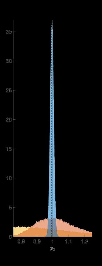
Challenges in Dynamical Systems Inference:
New Approaches for Parameter and Uncertainty Estimation

                                                                              Matthias Chung
                                                                       Department of Mathematics
                                                   Computational Modeling & Data Analytics Division
                                                                   Academy of Integrated Science
                                                                                     Virginia Tech
                                                                             mcchung@vt.edu
           wikipedia.com
                                                               January 2020 @ Universität Potsdam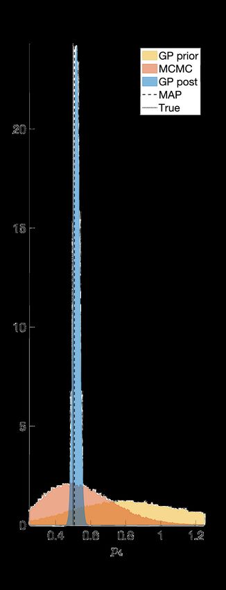
acknowledgment & funding

         DMS 1723005 & I/UCRC   R21 GM107683-01   NIFA: 2016-08687
         1650463

1 / 41                                                               mcchung@vt.edu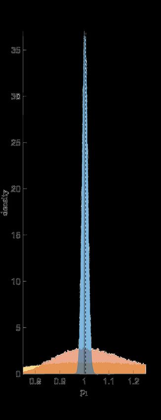
collaborators

         • John Bardsley, University of Montana
         • Mickael Binois, Argonne National Lab
         • Bobby Gramacy, Virginia Tech
         • Amber Smith, University of Tennessee, Memphis
         • Romcholo Macatula, Virginia Tech
         • Mihai Pop, University of Maryland College Park
         • Justin Krueger, Virginia Tech
         • Honghu Liu, Virginia Tech
         • Eldad Haber, University of British Columbia
         • Julianne Chung, Virginia Tech
         • Lars Ruthotto, Emory University

2 / 41                                                      mcchung@vt.edu
outline
          ``All models are wrong, but some are useful, ...
                                                     (George Box)

3 / 41                                                         mcchung@vt.edu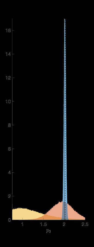
outline
          ``All models are wrong, but some are useful, ...
                                                     (George Box)
                   ... and some are dangerous.''
                                                    (Lenny Smith)

3 / 41                                                        mcchung@vt.edu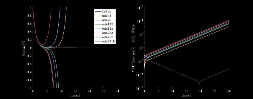
outline
``All models are wrong, but some are useful, ...
(George Box)
... and some are dangerous.''
(Lenny Smith)
Outline
À robust ODE/DDE solvers
Á dynamical systems parameter estimation
 surrogate data
à optimal experimental design
3 / 41 mcchung@vt.edu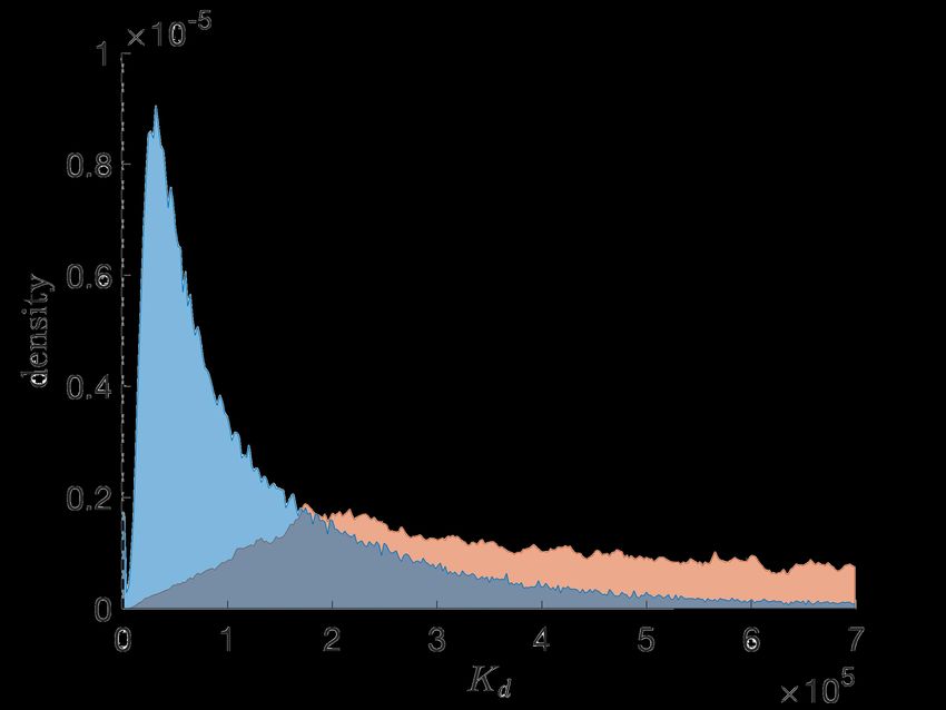
À robust lsfem solvers for
         • ordinary & delay differential equations (ODE/DDE)
         • initial & boundary value problems (IVP/BVP)
         • differential algebraic equations (DAE)

    G Hairer, SP Nørsett, and E Wanner. Solving Ordinary Differential Equations I: Nonstiff Problems. 2nd ed. Berlin: Springer, 1993.
4 / 41                                                                                                                                  mcchung@vt.edu
À robust lsfem solvers for
         • ordinary & delay differential equations (ODE/DDE)
         • initial & boundary value problems (IVP/BVP)
         • differential algebraic equations (DAE)
    Example y 0 = y − 2e−t , y(0) = 1 with exact solution y(t) = e−t

    Hairer, Nørsett, and Wanner 1993.
4 / 41                                                                 mcchung@vt.edu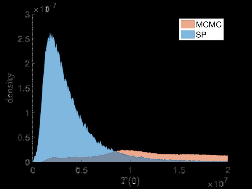
À ODE: Burlisch-Bock parameter estimation problem


                               0 0 1               0                                                      1
                             y = 2     y−                                                         y(0) =
                                 µ 0        (µ2 + ρ2 ) sin ρt                                             0
    t ∈ [0, 1] with µ = ρ = 15. Estimate true µ for data

    Hans Georg Bock. Recent advances in parameteridentification techniques for ode. In: Numerical treatment of inverse problems in differential
    and integral equations. Springer, 1983, pp. 95–121.
    R Bulirsch. Die Mehrzielmethode zur numerischen Lösung von nichtlinearen Randwertproblemen und Aufgaben der optimalen Steuerung. In:
    Report der Carl-Cranz-Gesellschaft 251 (1971).
5 / 41                                                                                                                                mcchung@vt.edu
À ODE: Burlisch-Bock parameter estimation problem
0 0 1 0 1
y = 2 y− y(0) =
µ 0 (µ2 + ρ2 ) sin ρt 0
t ∈ [0, 1] with µ = ρ = 15. Results using MCMC method
Bock 1983.
Bulirsch 1971.
5 / 41 mcchung@vt.eduÀ Hénon-Heiles Hamiltonian system
y1 −y3 − 2λy3 y4 y1 (0) 1
y2 −y4 − λ(y32 − y42 ) y2 (0) 1
=
y3
wrt.
y3 (0) = 0.18 1 , λ = 1 and t ∈ [0, 100, 000]
y1
y4 y2 y4 (0) 1
E Hairer and M Hairer. GniCodes—Matlab programs for geometric numerical integration. In: Frontiers in Numerical Analysis (Durham, 2002).
Universitext. Springer, Berlin, 2003, pp. 199–240.
6 / 41 mcchung@vt.eduÁ parameter estimation problem
d
parameter-to-model model-to-data
x y(x) m(y(x)) J (x, y, d) + R(x)
loss
prior knowledge/regularization
• x ∈ Rn parameter
• y : Rn → Y model, e.g., ODE, DDE, PDE
• m : Y → Rm , projection onto data, e.g., ODE evaluated at discrete
time points
• d ∈ Rm
• e.g., J (x) = km(y(x)) − dk22 , where k · k2 Euclidean norm
• R : Rn → R regularization/prior knowledge (e.g., sparsity k · k1 )
• Interpretation as MAP estimate in a Bayesian framework
7 / 41 mcchung@vt.eduÁ parameter estimation via principal differential analysis (PDA)
b = arg min km(y(t)) − dk22
x subject to y0 (t) = f (t, y(t); x), y(t0 ) = y0
x
"derivation":
M Chung, J Krueger, and M Pop. Identification of microbiota dynamics using robust parameter estimation methods. In: Mathematical
Biosciences 294 (2017), pp. 71–84.
Jim O Ramsay. Principal differential analysis: Data reduction by differential operators. In: Journal of the Royal Statistical Society. Series B
(Methodological) (1996), pp. 495–508.
A.A. Poyton, M.S. Varziri, K.B. McAuley, P.J. McLellan, and J.O. Ramsay. Parameter estimation in continuous-time dynamic models using
principal differential analysis. In: Comput. Chem. Eng. 30.4 (2006), pp. 698–708.
8 / 41 mcchung@vt.eduÁ parameter estimation via principal differential analysis (PDA)
(b b ) = arg min km(y(t)) − dk22 + λky0 (t) − f (t, y(t); x)k2L2
x, y subject to y(t0 ) = y0
x,y
"derivation":
1. relax ODE constraint
Chung, Krueger, and Pop 2017.
Ramsay 1996.
Poyton, Varziri, McAuley, McLellan, and Ramsay 2006.
8 / 41 mcchung@vt.eduÁ parameter estimation via principal differential analysis (PDA)
(b b) = arg min km(s(t; q))−dk22 +λks0 (t; q)−f (t, s(t; q); x)k2L2 ,
x, q subject to s(t0 ) = y0
x,q
"derivation":
1. relax ODE constraint
2. restrict to parameterized finite function space
Chung, Krueger, and Pop 2017.
Ramsay 1996.
Poyton, Varziri, McAuley, McLellan, and Ramsay 2006.
8 / 41 mcchung@vt.eduÁ parameter estimation via principal differential analysis (PDA)
(b b) = arg min km(s(t; q))−dk22 +λks0 (T; q)−f (T, s(T; q); x)k22
x, q subject to s(t0 ) = y0
x,q
"derivation":
1. relax ODE constraint
2. restrict to parameterized finite function space
3. discretize T = [T1 , . . . , TM ]>
advantages:
• simultaneous parameter and approximate ODE solve
• robustness in parameter estimates
Chung, Krueger, and Pop 2017.
Ramsay 1996.
Poyton, Varziri, McAuley, McLellan, and Ramsay 2006.
8 / 41 mcchung@vt.eduÁ generalized Lotka-Volterra simulation study
Consider the 4 state Lotka-Volterra system
y0 = diag (y) (r + Ay), y(0) = y0
with
2 0 −0.6 0 −0.2 5
1 0.6 0 −0.6 −0.2 4
r=
0 ,
A= , y0 =
3 .
0 0.6 0 −0.2
−3 0.2 0.2 0.2 0 2
Goal: Estimating x = [r; vec(A); y0 ] give data.
9 / 41 mcchung@vt.eduÁ data recovery
Average relative error:
80
1 X mj (y) − dj
er =
80 dj
j=1
Study 1 (0% noise):
er ≈ 0.0331
Study 2 (up to 10% noise):
er ≈ 0.0926
Study 3 (up to 25% noise):
dynamics vs. data
er ≈ 0.1511
10 / 41 mcchung@vt.eduÁ intestinal microbiota (interaction matrix and comparison)
PDA (A) versus published interaction matrix (B)
1. Blautia 5. Unclassified Lachnospiraceae
2. Barnesiella 6. Coprobacillus
3. Unclassified Mollicutes 7. Other
4. Undefined Lachnospiraceae
C G Buffie, I Jarchum, et al. Profound alterations of intestinal microbiota following a single dose of clindamycin results in sustained susceptibility
to Clostridium difficile-induced colitis. In: Infect. Immun. 80.1 (2012), pp. 62–73; R R Stein, V Bucci, et al. Ecological modeling from time-
series inference: insight into dynamics and stability of intestinal microbiota. In: PLoS Comput. Biol. 9.12 (2013), e1003388; C G Buffie,
V Bucci, et al. Precision microbiome reconstitution restores bile acid mediated resistance to Clostridium difficile. In: Nature 517.7533 (2015),
pp. 205–208.
11 / 41 mcchung@vt.edu Gaussian processes
A Gaussian process is a collection of random variables g(t); any fi-
nite number {g(ti )}m i=1 of which have a joint Gaussian distribution,
i.e., for finite t = [t1 , . . . , tm ]> ∈ Rm , the joint distribution is Gaus-
sian,
g(t) ∼ N ([µ(ti )]m m
i=1 , [κ(ti , tj )]i,j=1 )
e.g., random walk
C E Rasmussen and C K I Williams. Gaussian Process for Machine Learning. MIT press, 2006.
12 / 41 mcchung@vt.edu Gaussian process prior
Kernel κ(t, t̃) is real, symmetric, non-negative, integrable function
13 / 41 mcchung@vt.edu Gaussian process prior
Kernel κ(t, t̃) is real, symmetric, non-negative, integrable function
2
squared exponential kernel κ(t, t̃) = τ 2 exp − 2`12 t − t̃ 2 (τ = 1)
`2 = 0.01 (length scale parameter)
13 / 41 mcchung@vt.edu Gaussian process prior
Kernel κ(t, t̃) is real, symmetric, non-negative, integrable function
2
squared exponential kernel κ(t, t̃) = τ 2 exp − 2`12 t − t̃ 2 (τ = 1)
`2 = 0.001 (length scale parameter)
14 / 41 mcchung@vt.edu Gaussian process prior
Kernel κ(t, t̃) is real, symmetric, non-negative, integrable function
q !ν q !
21−ν 2ν|t−t̃| 2ν|t−t̃|
Matérn kernel κ(t, t̃) = Γ(ν) ` Kν `
Γ Gamma function, Kν modified Bessel function, ν = 1/2
15 / 41 mcchung@vt.edu Gaussian process prior
Kernel κ(t, t̃) is real, symmetric, non-negative, integrable function
q !ν q !
21−ν 2ν|t−t̃| 2ν|t−t̃|
Matérn kernel κ(t, t̃) = Γ(ν) ` Kν `
Γ Gamma function, Kν modified Bessel function, ν = 3/2
16 / 41 mcchung@vt.edu conditional distribution/prediction
d 0m Σt ΣtT
joint distribution at t and T: ∼N ,
g 0M ΣTt ΣT
conditional (predictive) distribution
(g|d) ∼ N (µ, Σ), with µ = ΣTt Σ−1
t d and Σ = ΣT − ΣTt Σ−1
t ΣtT
17 / 41 mcchung@vt.edu surrogate problem
For predictive Gaussian process g ∼ N (µ, Σ) for given data
(t, d) and model y solve
b = arg min km(y(t, x)) − gk2Σ−1 + R(x)
x
x
Algorithm: sampled GP weighted least squares
input: model y, projection m, µ, Σ, initial guess x0
1: parallel for j = 1 to J do
2: sample gj from Gaussian process N (µ, Σ)
3: solve xbj = arg minx km(y(t, x)) − gj k2Σ−1 + R(x)
4: end parallel for
output: {b xj }Jj=1
M Chung, M Binois, et al. Parameter and Uncertainty Estimation for Dynamical Systems Using Surrogate Stochastic Processes. In: arXiv
preprint arXiv:1802.00852 (2018).
18 / 41 mcchung@vt.edu motivating example: Lotka-Volterra & model
y10 = −y1 + x1 y1 y2 y20 = y2 − x2 y1 y2
unknow parameter x = [x1 , x2 , y1 (0), y2 (0)]>
Matthias Chung, Mickaël Binois, et al. Parameter and uncertainty estimation for dynamical systems using surrogate stochastic processes. In:
SIAM Journal on Scientific Computing 41.4 (2019), A2212–A2238.
19 / 41 mcchung@vt.edu Lotka-Volterra UQ
marginal 1D densities with GP and with MCMC
20 / 41 mcchung@vt.edu motivating example: influenza virus data & model
T 0 = −βT V
I10 = βT V − κI1
δI2
I20 = κI1 −
Kd + I2
0
V = ρI2 − cV
• T target cells • ρ virus production rate
• I1 and I2 infected cells • c clearance rate
• V virus • δ density dependent clearance
• β ``contact rate'' • Kd half-saturation constant
• κ rate (eclipse)
Chung, Binois, et al. 2019.
21 / 41 mcchung@vt.edu influenza virus GP 22 / 41 mcchung@vt.edu
 influenza virus GP 23 / 41 mcchung@vt.edu
 influenza virus GP
marginal 1D densities with GP and with MCMC
24 / 41 mcchung@vt.eduà optimal experimental design framework
J (x) R(x)
z }| { z }| {
x
b 1
= arg min 2 ky( x) − d k 2Γ−1 + 2 kLxk22
1
x ε
subject to Ce x − ce = 0 and Ci x − ci ≥ 0 ,
• Ce , Ci , ce , ci constraints
E Haber, L Horesh, and L Tenorio. Numerical methods for experimental design of large-scale linear ill-posed inverse problems. In: Inverse
Problems 24.5 (2008), p. 055012.
M Chung and E Haber. Experimental Design for Biological Systems. In: SIAM Journal on Control and Optimization 50.1 (2012), pp. 471–489.
25 / 41 mcchung@vt.eduà optimal experimental design framework
J (x) R(x)
z }| { z }| {
2
b(p) = arg min 12 ky(p, x) − d(p)k 2Γ−1 (p) +
x 1
2 kLxk2
x ε
subject to Ce x − ce = 0 and Ci x − ci ≥ 0 ,
• Ce , Ci , ce , ci constraints
• p ∈ Ω design parameter (Ω set of feasible design parameter)
Haber, Horesh, and Tenorio 2008.
Chung and Haber 2012.
25 / 41 mcchung@vt.eduà optimal experimental design framework
Bayes risk approach (average design)
min J (p) = 1
2 x(p) − xtrue k22 + Rp (p)
E kb subject to
p∈Ω
J (x) R(x)
z }| { z }| {
2
b(p) = arg min 12 ky(p, x) − d(p)k 2Γ−1 (p) +
x 1
2 kLxk2
x ε
subject to Ce x − ce = 0 and Ci x − ci ≥ 0 ,
• Ce , Ci , ce , ci constraints
• p ∈ Ω design parameter (Ω set of feasible design parameter)
• E expected value (sampling of expected value via training data
xjtrue , with j = 1, . . . , M )
• Rp regularization (cost) on design parameter p
Haber, Horesh, and Tenorio 2008.
Chung and Haber 2012.
25 / 41 mcchung@vt.eduà optimal experimental design framework
Bayes risk approach (average design)
min J (p) = 1
2 x(p) − xtrue k22 + β||p||1
E kb subject to
p∈Ω
J (x) R(x)
z }| { z }| {
2
b(p) = arg min 12 ky(p, x) − d(p)k 2Γ−1 (p) +
x 1
2 kLxk2
x ε
subject to Ce x − ce = 0 and Ci x − ci ≥ 0 ,
• Ce , Ci , ce , ci constraints
• p ∈ Ω design parameter (Ω set of feasible design parameter)
• E expected value (sampling of expected value via training data
xjtrue , with j = 1, . . . , M )
• Rp regularization (cost) on design parameter p
Haber, Horesh, and Tenorio 2008.
Chung and Haber 2012.
25 / 41 mcchung@vt.eduà Exponential growth
y 0 = xy unknown parameter x
pmax
j pj = 0
samples = 10, discretization 101, no noise, and L = 0.1In
26 / 41 mcchung@vt.eduà Exponential growth
y 0 = xy unknown parameter x
aMSE
# of nonzeros
27 / 41 mcchung@vt.eduà Logistic growth
y 0 = x1 y − x2 y 2 unknown parameter x = [x1 , x2 ]>
pmax
j pj = 0
samples = 20, discretization 101, no noise, and L = 0.1In
28 / 41 mcchung@vt.eduà Logistic growth
y 0 = x1 y − x2 y 2 unknown parameter x = [x1 , x2 ]>
aMSE
# of nonzeros
29 / 41 mcchung@vt.eduà Lotka-Volterra
y10 = x1 y1 − x2 y1 y2
x = [x1 , x2 , x3 , x4 ]>
y20 = −x3 y2 + x4 y1 y2
pmax
j pj = 0
samples = 10, discretization 202, no noise, and L = 0.1In
30 / 41 mcchung@vt.eduà Lotka-Volterra
y10 = x1 y1 − x2 y1 y2
x = [x1 , x2 , x3 , x4 ]>
y20 = −x3 y2 + x4 y1 y2
aMSE
# of nonzeros
31 / 41 mcchung@vt.eduà intravenous glucose tolerance test (IVGTT) 32 / 41 mcchung@vt.edu
à glucose minimal model
   Minimal Model
                                   Ġ(t) = −x1 + X(t)G(t) + x1 Gb
                                    ˙ = −γ max(G(t) − h, 0)t − n(I(t) − Ib )
                                    I(t)
                                   Ẋ(t) = −x2 X(t) + x3 (I(t) − Ib )
           G, I, X        blood glucose, plasma insulin, effective insulin
            Gb , I b      basal level of glucose and insulin
                  γ       pancreatic insulin release rate
                  h       pancreatic threshold
                 n        degradation rate of insulin
                x1        glucose effectiveness
                x2        degradation rate of effective insulin
                x3        stimulation sensitivity of insulin
   R N Bergman, L S Phillips, and C Cobelli. Physiologic evaluation of factors controlling glucose tolerance in man: measurement of insulin
   sensitivity and beta-cell glucose sensitivity from the response to intravenous glucose. In: The Journal of clinical investigation 68.6 (1981),
   pp. 1456–1467.
33 / 41                                                                                                                                 mcchung@vt.edu
à minimal model
54 samples, discretization 241
34 / 41 mcchung@vt.eduà IVGTT: sparsity vs. error 35 / 41 mcchung@vt.edu
à IVGTT: proposed design

36 / 41                    mcchung@vt.edu
à tomography
                                y                                                   d(θ) = TR(θ)xtrue + ε(θ)
                                         x-ray source
                                                                       • xtrue ∈ Rn true object
                                                                       • θ angle
                                                                       • R(θ) ∈ Rn×n rotation of object
                                                            θ          • T ∈ Rnr ×n transmission process
                                                             x
                                                                        Where and how often should be
                                                                        measured for good recovery?

                                                                  Design constraints
                                                                   • time                                  • cost
                  detector                                          • health risk                          • limited resources
    L Ruthotto, J Chung, and M Chung. Optimal Experimental Design for Inverse Problems with State Constraints. In: SIAM Journal on Scientific
    Computing 40.4 (2018), B1080–B1100.
37 / 41                                                                                                                            mcchung@vt.edu
à tomography results: rectangles
unconstrained equality constrained non-negativity constrained box constrained
reconstructions f̂
residuals f̂ − ftrue
intuitive optimal angles [0, 90] [0, 90] (non-negative) [0, 90] (box)
38 / 41 mcchung@vt.eduà tomography results: pentagons
reconstructions f̂
residuals f̂ − ftrue unconstrained equality constrained non-negativity constrained box constrained
intuitive optimal angles [27, 63, 99, 135, 171]
[25, 64, 99, 136, 171] (non-negative) [27, 62, 99, 134, 171] (box)
39 / 41 mcchung@vt.eduà tomography results: Shepp-Logan phantom
unconstrained equality constrained non-negativity constrained box constrained
reconstructions f̂
error f̂ − ftrue
40 / 41 mcchung@vt.eduà conclusion & outlook
Take-home message
• flexible and robust differential equation solvers
• efficient parameter estimation method using PDA
• robust parameter estimation via surrogate data
• new computational framework for optimal experimental design
Outlook
• computational methods for finite element methods for
ODE/DDE/DAE
• Gaussian processes for ODE PE, inverse problems, model
reduction, missing data problems
• apply OED to various system setups
Thank you for your attention!
41 / 41 mcchung@vt.eduà References I
Bardsley, J M, A Solonen, H Haario, and M Laine. Randomize-then-optimize: A
method for sampling from posterior distributions in nonlinear inverse problems.
In: SIAM Journal on Scientific Computing 36.4 (2014), A1895–A1910.
Bergman, R N, L S Phillips, and C Cobelli. Physiologic evaluation of factors
controlling glucose tolerance in man: measurement of insulin sensitivity and
beta-cell glucose sensitivity from the response to intravenous glucose. In: The
Journal of clinical investigation 68.6 (1981), pp. 1456–1467.
Bock, Hans Georg. Recent advances in parameteridentification techniques for ode.
In: Numerical treatment of inverse problems in differential and integral
equations. Springer, 1983, pp. 95–121.
42 / 41 mcchung@vt.eduà References II
Buffie, C G, V Bucci, R R Stein, P T McKenney, L Ling, A Gobourne, D No,
H Liu, M Kinnebrew, A Viale, E Littmann, M R van den Brink, R R Jenq,
Y Taur, C Sander, J R Cross, N C Toussaint, J B Xavier, and E G Pamer.
Precision microbiome reconstitution restores bile acid mediated resistance to
Clostridium difficile. In: Nature 517.7533 (2015), pp. 205–208.
Buffie, C G, I Jarchum, M Equinda, L Lipuma, A Gobourne, A Viale, C Ubeda,
J Xavier, and E G Pamer. Profound alterations of intestinal microbiota following
a single dose of clindamycin results in sustained susceptibility to Clostridium
difficile-induced colitis. In: Infect. Immun. 80.1 (2012), pp. 62–73.
Bulirsch, R. Die Mehrzielmethode zur numerischen Lösung von nichtlinearen
Randwertproblemen und Aufgaben der optimalen Steuerung. In: Report der
Carl-Cranz-Gesellschaft 251 (1971).
43 / 41 mcchung@vt.eduà References III
Calvetti, D and E Somersalo. Introduction to Bayesian Scientific Computing: Ten
Lectures on Subjective Computing. New York: Springer, 2007. isbn:
0387733930.
Chung, M, M Binois, RB Gramacy, DJ Moquin, AP Smith, and AM Smith.
Parameter and Uncertainty Estimation for Dynamical Systems Using Surrogate
Stochastic Processes. In: arXiv preprint arXiv:1802.00852 (2018).
Chung, M and E Haber. Experimental Design for Biological Systems. In: SIAM
Journal on Control and Optimization 50.1 (2012), pp. 471–489.
Chung, M, J Krueger, and M Pop. Identification of microbiota dynamics using
robust parameter estimation methods. In: Mathematical Biosciences 294
(2017), pp. 71–84.
44 / 41 mcchung@vt.eduà References IV
Chung, Matthias, Mickaël Binois, Robert B Gramacy, Johnathan M Bardsley,
David J Moquin, Amanda P Smith, and Amber M Smith. Parameter and
uncertainty estimation for dynamical systems using surrogate stochastic
processes. In: SIAM Journal on Scientific Computing 41.4 (2019),
A2212–A2238.
Haber, E, L Horesh, and L Tenorio. Numerical methods for experimental design of
large-scale linear ill-posed inverse problems. In: Inverse Problems 24.5 (2008),
p. 055012.
Hairer, E and M Hairer. GniCodes—Matlab programs for geometric numerical
integration. In: Frontiers in Numerical Analysis (Durham, 2002). Universitext.
Springer, Berlin, 2003, pp. 199–240.
Hairer, G, SP Nørsett, and E Wanner. Solving Ordinary Differential Equations I:
Nonstiff Problems. 2nd ed. Berlin: Springer, 1993.
45 / 41 mcchung@vt.eduà References V
Poyton, A.A., M.S. Varziri, K.B. McAuley, P.J. McLellan, and J.O. Ramsay.
Parameter estimation in continuous-time dynamic models using principal
differential analysis. In: Comput. Chem. Eng. 30.4 (2006), pp. 698–708.
Ramsay, Jim O. Principal differential analysis: Data reduction by differential
operators. In: Journal of the Royal Statistical Society. Series B (Methodological)
(1996), pp. 495–508.
Rasmussen, C E and C K I Williams. Gaussian Process for Machine Learning. MIT
press, 2006.
Ruthotto, L, J Chung, and M Chung. Optimal Experimental Design for Inverse
Problems with State Constraints. In: SIAM Journal on Scientific Computing
40.4 (2018), B1080–B1100.
Smith, R C. Uncertainty Quantification: Theory, Implementation, and
Applications. Vol. 12. SIAM, 2013.
46 / 41 mcchung@vt.eduà References VI
Stein, R R, V Bucci, N C Toussaint, C G Buffie, G Rätsch, E G Pamer, C Sander,
and J B Xavier. Ecological modeling from time-series inference: insight into
dynamics and stability of intestinal microbiota. In: PLoS Comput. Biol. 9.12
(2013), e1003388.
Tenorio, L. An Introduction to Data Analysis and Uncertainty Quantification for
Inverse Problems. Vol. 3. SIAM, 2017.
Wahba, G. Smoothing noisy data with spline functions. In: Numerische
Mathematik 24.5 (1975), pp. 383–393.
47 / 41 mcchung@vt.eduYou can also read


