Classification of Daily Irradiance Profiles and the Behaviour of Photovoltaic Plant Elements: The Effects of Cloud Enhancement
←
→
Page content transcription
If your browser does not render page correctly, please read the page content below
applied
              sciences
Article
Classification of Daily Irradiance Profiles and the Behaviour of
Photovoltaic Plant Elements: The Effects of Cloud Enhancement
Isabel Santiago * , Jorge Luis Esquivel-Martin, David Trillo-Montero, Rafael Jesús Real-Calvo
and Víctor Pallarés-López

                                           Department of Electronic and Computer Engineering, Campus de Rabanales, University of Córdoba,
                                           14071 Córdoba, Spain; jorgel.esquivelm@gmail.com (J.L.E.-M.); ma2trmod@uco.es (D.T.-M.);
                                           el1recar@uco.es (R.J.R.-C.); el1palov@uco.es (V.P.-L.)
                                           * Correspondence: el1sachi@uco.es; Tel.: +34-957-218699

                                           Abstract: In this work, the automatic classification of daily irradiance profiles registered in a photo-
                                           voltaic installation located in the south of Spain was carried out for a period of nine years, with a
                                           sampling frequency of 5 min, and the subsequent analysis of the operation of the elements of the
                                           installation on each type of day was also performed. The classification was based on the total daily
                                           irradiance values and the fluctuations of this parameter throughout the day. The irradiance profiles
                                           were grouped into nine different categories using unsupervised machine learning algorithms for
                                           clustering, implemented in Python. It was found that the behaviour of the modules and the inverter
                                           of the installation was influenced by the type of day obtained, such that the latter worked with
                                           a better average efficiency on days with higher irradiance and lower fluctuations. However, the

                                    modules worked with better average efficiency on days with irradiance fluctuations than on clear
Citation: Santiago, I.;                    sky days. This behaviour of the modules may be due to the presence, on days with passing clouds, of
Esquivel-Martin, J.L.; Trillo-Montero,     the phenomenon known as cloud enhancement, in which, due to reflections of radiation on the edges
D.; Real-Calvo, R.J.; Pallarés-López, V.   of the clouds, irradiance values can be higher at certain moments than those that occur on clear sky
Classification of Daily Irradiance         days, without passing clouds. This is due to the higher energy generated during these irradiance
Profiles and the Behaviour of              peaks and to the lower temperatures that the module reaches due to the shaded areas created by the
Photovoltaic Plant Elements: The           clouds, resulting in a reduction in its temperature losses.
Effects of Cloud Enhancement. Appl.
Sci. 2021, 11, 5230. https://doi.org/      Keywords: irradiance daily profiles; unsupervised machine learning; clustering algorithm; perfor-
10.3390/app11115230
                                           mance ratio; photovoltaic module efficiency; inverter efficiency; cloud enhancement; irradiance en-
                                           hancement
Academic Editor: Manuela Sechilariu

Received: 28 April 2021
Accepted: 1 June 2021
                                           1. Introduction
Published: 4 June 2021
                                                 Renewable energy sources, which are clean and inexhaustible resources that are used
Publisher’s Note: MDPI stays neutral
                                           for electricity generation through different technologies, are currently playing a crucial role
with regard to jurisdictional claims in
                                           in the race to achieve some of the Sustainable Development Goals of the United Nations [1],
published maps and institutional affil-    such as Goal 7, which aims to ensure access to affordable, reliable, sustainable and modern
iations.                                   energy for all. The target set by the International Renewable Energy Agency (IRENA)
                                           is to produce 57% of the world’s energy from renewable sources by 2030, up from 26%
                                           today, more than doubling the existing share, so this decade is considered to be the one
                                           in which renewable energies will drive the global energy transformation [2]. Even more
Copyright: © 2021 by the authors.
                                           ambitious are the objectives proposed by European countries through the European Green
Licensee MDPI, Basel, Switzerland.
                                           Deal, whose objective, in the fight against the threat of climate change and environmental
This article is an open access article
                                           degradation, is that there will be no net emissions of greenhouse gases by 2050 [3].
distributed under the terms and                  Within renewable energies, a wide range of typologies can be found, and the one
conditions of the Creative Commons         that currently has the highest growth rate is photovoltaic (PV) energy [4]. In 2019, this
Attribution (CC BY) license (https://      was the most installed energy source among both renewables and non-renewable energies,
creativecommons.org/licenses/by/           accounting for 40% of new global capacity [4–6]. Globally, new PV capacity in 2019 was
4.0/).                                     115 GW, an increase of 12% compared to 2018, giving a cumulative total of 627 GW. These

Appl. Sci. 2021, 11, 5230. https://doi.org/10.3390/app11115230                                             https://www.mdpi.com/journal/applsci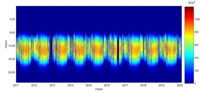
Appl. Sci. 2021, 11, 5230                                                                                             2 of 28

                            figures were obtained due to the growth that took place on all continents, highlighting the
                            increase in some countries such as China (30 GW), USA (13 GW), India (10 GW) and Japan
                            (7 GW). In the European Union, PV energy saw very significant growth, with 16.7 GW
                            installed, an increase of 104 % compared to 2018 (8.2 GW), the strongest growth since
                            2010 [4,7,8]. This increase in the installed capacity of renewable energies, and in particular
                            the increase in PV power, has allowed around a third of the world’s electricity generation
                            to take place without fossil fuels and therefore with zero emissions [4].
                                  With this rate of expansion, PV technology, which has come to be considered the
                            world’s fastest growing power generation source and a driving force behind energy tran-
                            sition in some countries, is expected to further increase in installed capacity in the near
                            future [4,7,9,10]. In this regard, renewable energies in general, and PV in particular, have in
                            recent years considerably increased their role in the generation mix of different countries,
                            and their presence has led to changes in grid operation strategies [6]. These policies must
                            continue to evolve in the future so that renewables energies form the basis of electricity
                            generation and of the transition towards greater decarbonisation of sectors such as the
                            demand for building power, air conditioning and transport [3,11–13].
                                  Nowadays, the main disadvantage of renewable energy sources is their manageability
                            or dispatchability, as the energy they produce is conditioned by the randomness of the
                            weather, giving rise to rapid variations in their production [14]. If electricity generated
                            from renewable sources cannot be stored at a reasonable cost, its penetration in the grid is
                            limited, and the share of renewable energy in the generation mix will be even more difficult
                            to increase.
                                  For a better manageability of solar PV installations, which enables an increase in their
                            penetration in the power grid, it is important to know in advance the electrical energy
                            that is to be produced, in order to be able to predict more accurately how the product can
                            be delivered in the time intervals considered in the daily and intraday energy markets.
                            The need for better forecasting has for years increased interest in various solutions, and
                            different authors have used different techniques [15–21], such as time series prediction
                            with statistical and learning methods [22], or atmospheric modelling with the analysis of
                            sky satellite images and the study of cloud propagation [23]. All these models are based on
                            meteorological and/or historical production data. Among all of them, the categorisation of
                            solar irradiance data is one of the earliest applied techniques [24], and in the literature there
                            are many authors who have analysed and predicted the behaviour of irradiance profiles,
                            using various procedures [24–27].
                                  In order to characterise daily irradiance profiles, several authors define a series of
                            indices, such as the clearness index, which represents the proportion of measured irradiance
                            and theoretical irradiance under clear sky conditions. There is also the variability or
                            intermittency index, or the fractal dimension [28–30], which are parameters that take
                            into account the deviation of the actual irradiance values from clear sky conditions. For
                            their characterisation, the irradiance data recorded over time can be used directly or,
                            alternatively, a transformation of these temporal data to the frequency domain can be
                            performed beforehand [24]. All these types of data can be used to make classifications,
                            in order to extract different types of days, and group those types of daily profiles with
                            similar behaviour. Different authors use different methods to make these classifications,
                            considering a greater or a lesser number of types of days [24,25,31–37].
                                  Although obviously the production of a PV plant at each moment in time will depend
                            on the amount of irradiance received by the solar panels and the temperature at which
                            they operate, the meteorological conditions that occur throughout the day, such as the
                            variation in ambient temperature and wind speed, as well as cloud cover and the speed at
                            which clouds are moving, generally determine the operation conditions and the behaviour
                            of the plant’s components, so that the efficiency and yield values of both the modules
                            and the inverters are modified throughout the day, and from one day to the next [38,39].
                            This means that the ability of the components of the PV system to convert the received
                            irradiance into electricity is not constant, but is influenced by the type of day that occurs.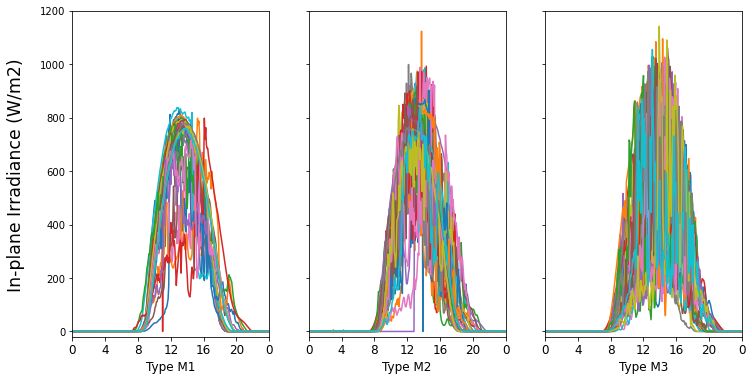
Appl. Sci. 2021, 11, 5230                                                                                            3 of 28

                                 In this context, one of the main objectives of this work was to apply a classification
                            algorithm to a nine-year history of records of the global irradiance received by the PV
                            modules of a solar installation, in order to automatically find patterns or types of days.
                            Once the days were classified according to the daily irradiance profiles, the dependence
                            between the patterns of days found and the operation and performance of the PV plant
                            components were also analysed, which is one of the main contributions of this paper. To
                            obtain the different types of days, a clustering method was used, within the unsupervised
                            automatic machine learning techniques, making use of the existing tools in the Python
                            programming language. The method used in this work stands out for its simplicity and
                            ease of application, and requires almost no changes to the irradiance data measured at the
                            PV plant, so no data filtering or transformation are required [24]. If the weather forecast
                            is known in advance, it will be possible to know beforehand the type of day that is going
                            to take place, and from the results found, it will be possible to know what the plant’s
                            behavioural interval will be, which will obviously influence its production. Once the
                            behaviour of the installation components were obtained on each type of day, another of the
                            aims of this work was to show the reasons for the variation in this behaviour on different
                            types of days. To this end, an analysis of the operation of its elements on clear sky days was
                            carried out, comparing it with that obtained on days with a greater presence of fluctuations.
                                 On these non-stable days there may be peaks of irradiance higher than the values
                            registered on clear sky days, due to the phenomenon known as cloud enhancement (CE) or
                            irradiance enhancement (IE) [40], and the presence of these events was also analysed in
                            this paper. According to Jarvela et al. [41], although the CE phenomenon is well known, its
                            effects on actual PV systems has not been thoroughly studied.
                                 The rest of the paper is organised as follows. Section 2 presents the methodology
                            employed and the characteristics of the data used in the study, Section 3 shows and
                            discusses the results obtained, and Section 4 shows the conclusions extracted from them.

                            2. Materials and Methods
                            2.1. Types of Algorithms Used for the Classification
                                 In this work, the classification of daily global irradiance profiles was carried out using
                            machine learning algorithms, which is the science of programming computers so that they
                            can learn or extract information from data, without being explicitly programmed. Within
                            machine learning, we are going to use a technique belonging to the so-called unsupervised
                            learning, which in general refers to methods in which the model is adjusted to observations.
                            Contrary to what happens in the so-called supervised learning techniques, in this case
                            there are no training data made up of input and output data, which enable us to provide a
                            priori the solution to the problem. The unsupervised learning techniques do not need an
                            “expert” intervention that provides known output data to the algorithm, offering a prior
                            knowledge of the result to be obtained, but only has input data, and the model is able to
                            find hidden structure in its inputs without knowledge of outputs [15,35]. Within these
                            unsupervised learning techniques, clustering algorithms were applied, whose objective is
                            to divide the data set into different groups of elements with similar characteristics, in such
                            a way that the objects grouped in the same group or cluster have similar characteristics and
                            that these characteristics are also different from those of the objects in the other groups.
                                 The classification algorithm chosen, from among the many existing ones, was the so-
                            called k-means. This one, developed by MacQueen in 1967, is a well-known and commonly
                            used partitional clustering algorithm [15,32,42]. Although it is not very well suited to
                            irregularly shaped groups, it was chosen because it is well suited to a large number of
                            samples, which is the case for the data used in this paper. This clustering method has
                            the advantage of creating averaged groups, while other clustering algorithms (such as
                            hierarchical clustering) tend to perform better in identifying the outliers [43]. For its
                            application it is required that the number of clusters, k, must be specified in advance.
                                 This k-means method groups the data by trying to separate the samples into k groups
                            of equal variance, minimising within each group the criterion known as inertia or sum of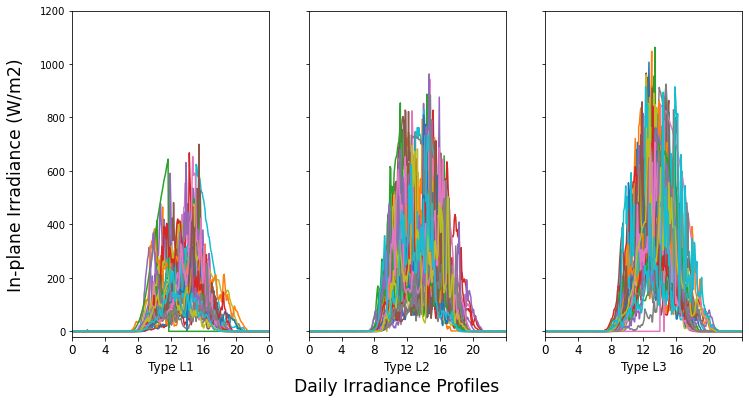
Appl. Sci. 2021, 11, 5230                                                                                               4 of 28

                            squares. The algorithm divides a number n of samples x, into a number of distinct groups
                            (k), and each of these groups is described by the mean µj of the samples in the group. This
                            average is known as the centre or centroid of the cluster, and generally they do not have to
                            be points of x, but must lie in the same space. The algorithm aims to choose centres that
                            minimise the inertia or sum of squares within the cluster, which is the Euclidean distance,
                            and is governed by the following expression,
                                                                   n
                                                                  ∑ µmin
                                                                      j ∈C
                                                                           (k xi − µ j k2 ),                               (1)
                                                                  i =0

                                  In general terms, the algorithm has three fundamental steps. The first step is based on
                            choosing k samples from the data set n, which would be the cluster centres at the beginning.
                            After initialisation, the algorithm consists of a loop between the next two steps. The second
                            step assigns each data item x to its nearest centre, while the third step creates new centres
                            by taking the average of the values of all samples assigned to the previous centre. The
                            algorithm will repeat steps two and three until the centres do not change significantly.
                                  For the initialisation of the centres, the k-means++ method was used in this work,
                            which distributes the initial centres so that they are generally distant from each other, in
                            order to try to prevent the algorithm from converging to a local, and therefore not optimal,
                            minimum. In this way, better results are obtained than by random initialisation.
                                  When performing point-to-point classifications, the Euclidean distance is used as
                            the base metric (Equation (1)), but for grouping time series into similar groups, this type
                            of metric is not the most appropriate. In this work, a distance metric dedicated to time
                            series, the so-called Dynamic Time Warping (DTW), was used, which is an algorithm for
                            measuring the similarity between two temporal linear sequences. DTW is an algorithm
                            for finding an optimal alignment between two sequences and a useful distance metric,
                            which possesses the capacity to cope with changes in data over time. The DTW Barycentre
                            Averaging (DBA) algorithm minimises the sum of the squared DTW distance between the
                            barycentre and the series in the group. As a result, the centroids have an average shape
                            that mimics the shape of the group members, regardless of where temporal changes occur
                            among the samples [44–47].
                                  Given two time series x = (x0 , . . . , xn ) and y = (y0 , . . . , ym ), with lengths n and m
                            respectively, the distance DTW from x to y is thus stated as an optimisation problem,
                            such that,                                          s
                                                         DTW ( x, y) = minπ         ∑        d ( x i , y j )2 ,            (2)
                                                                                   (i,j)€π

                            where d is the Euclidean distance between two points in the series and π = [π0 , . . . , πk ] is
                            a path that satisfies a number of properties. On the one hand, πk = (ik , jk ) represents pairs
                            of indices such that 0 ≤ ik < n and 0 ≤ jk < m. As boundary conditions π0 = (0, 0) and
                            πk = (n − 1, m − 1) are considered. As a continuity condition, it is stated that for all k > 0,
                            if πk = (ik , jk ) and πk−1 = (ik−1 , jk−1 ), it has to be fulfilled that ik−1 ≤ ik ≤ ik−1 + 1 and
                            jk−1 ≤ jk ≤ jk−1 + 1. Therefore, the path is a temporal alignment of time series such that
                            Euclidean distance between aligned or resampled time series is minimal [48].
                                  In this way, the k-means clustering method applied to time series, in this case applied
                            to daily irradiance profiles, using the DTW metric, created groups of irradiance daily
                            profiles with similar shapes, and the centres or centroids of the clusters were calculated as
                            barycentres or average sequences of a group of irradiance time series considered within
                            the same group.

                            2.2. Software Used to Apply the Classification
                                  To implement the above algorithm, the Python programming language was used. It
                            is a general-purpose, freely distributed, interpreted, multi-paradigm, multi-platform and
                            dynamically typed language. It owes its popularity to the large number of libraries and
                            functions available, with a great technical support thanks to a large community of users.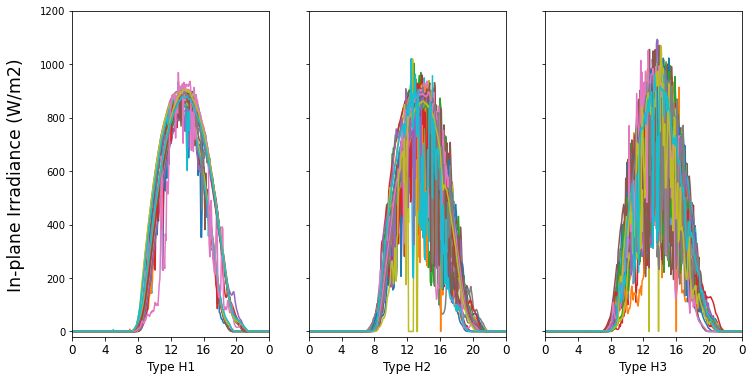
Appl. Sci. 2021, 11, 5230                                                                                            5 of 28

                            Anaconda, which is a Python distribution, was used for its management, and it was used in
                            the Windows environment. The main Python library used was Scikit-learn, which contains
                            state-of-the-art machine learning algorithms, as well as exhaustive documentation on each
                            one [49,50]. This library contains the clustering algorithms used in this work, which are
                            available in its module sklearn.clusters. ts-learn was also used, which is a general-purpose
                            machine learning Python library for time series, as is the case of the data analysed in this
                            work, and from which the modules tslearn.utils y tslearn.clustering [48] were mainly used.
                            The latter module offers the option of using DTW as the central metric in the k-means
                            algorithm, leading to better clusters and centroids in the case of this study. Scikit-learn
                            also relies on other Python packages that were used, such as NumPy, which is a library for
                            scientific computing, necessary for processing data in the form of arrays [51]; SciPy, which
                            has a collection of functions for scientific computing and on which Scikit-learn is based to
                            implement its algorithms [52]. Pandas, the library needed to manage, modify and operate
                            the files and data processed, was also used [53], and for the graphical representation of the
                            results of the algorithm, the library Matplotlib was used [54].

                            2.3. Monitored Data and Specifications of the Analysed PV System
                                 A set of 36 PV modules connected to an inverter were the elements used to carry out
                            the analysis shown in this paper. They belong to a PV installation located on the rooftop
                            of a building in the city of Cordoba (37◦ 530 0000 N, 4◦ 460 0000 O), in the south of Spain. The
                            modules, from BP, are made of polycrystalline silicon and have a peak power of 165 W.
                            Their characteristics are listed in Table 1. The modules are configured as three strings in
                            parallel, with 12 modules connected in series in each of them, and they are mounted on an
                            open frame with 30◦ of inclination and 18◦ of azimuth. The inverter to which the modules
                            are connected is from SMA, model SMC-100, and its specifications are shown in Table 2.

                            Table 1. General characteristics of the installation and its PV modules.

                                                                                                 Specifications
                                    Number of modules per inverter                                36 = 12 × 3
                                             Module model                                              BP-3165
                                         PV module peak power                                          165 W
                                       Number of cells per module                                        72
                                       Surface area of each module                              1,573,790 mm2
                                             PV cell surface                                   125 mm·125 mm
                                           Useful module area                                          1125 m2
                                     Power of modules per inverter                                     5940 W
                                      Power temperature coefficient                          −(0.5 ± 0.005) %/◦ C
                                      Temperature coefficient of Isc                         (0.065 ± 0.015) %/◦ C
                                     Temperature coefficient of Voc                          −(160 ± 20) mV/◦ C
                                                  NOCT                                           47 ◦ C ± 2 ◦ C
                                        Open-circuit voltage (Voc)                                     44.2 V
                                   Voltage at maximum power (Vmax)                                     35.2 V
                                        Short-circuit current (Isc)                                     5.2 A
                                    Current maximum power (Imax)                                        4.7 A
Appl. Sci. 2021, 11, 5230 6 of 28
Table 2. Inverter characteristics.
Specifications
Inverter model SMA SMC-5000
Maximum performance 96%
European performance >95.1%
Maximum input current 26 A
Maximum dc voltage 600 V
Maximum dc power 5750 W
PV voltage range, MPP 246–480 V
Number of MPPT 1
Maximum output current 26 A
Maximum nominal ac power 5000 W
Maximum ac power 5500 W
The data acquisition system of the PV installation is integrated in the inverter. The
measured parameters were stored with a frequency of 5 min, and they correspond to an
average value of each parameter in this time interval.
The irradiance values analysed in this work, which correspond to the global tilted irra-
diance (GTI), were collected by an equipment called Sunny SensorBox, from the company
SMA, to which the sensor of this parameter was connected, which was a calibrated PV ASI
amorphous cell, with a measurement range of 0 to 1500 W/m2 , an accuracy of ±8% and a
resolution of 1 W/m2 . This irradiance sensor was installed next to the PV modules, with the
same orientation and inclination, so that the recorded irradiance values would represent
those received by the PV panels. During the nine years of operation, a degradation of the
cell was detected, resulting in a decrease of 1.8% in the recorded irradiance data, which is
a percentage lower than the accuracy given by the sensor manufacturer. In addition, this
equipment also collected measurements from two temperature sensors. One of them, a
PT-100M sensor, with a range of −20 to +110 ◦ C, was used to measure the temperature of
the modules. Its accuracy and its resolution specified by the manufacturer were ±0.5 ◦ C
and 0.1 ◦ C, respectively. The other, a PT-100M-NR sensor, was used for measuring the
ambient temperature, which had the same characteristics as the previous one, but with
an accuracy of ±0.7 ◦ C given by the manufacturer. Assuming effects of decoupling and
stability for these sensors, the error in temperature measurements can be considered ±1 ◦ C.
The SensorBox and the inverter were connected via RS485 to a device called Sunny-
Webbox from SMA. It is a device with a central communications unit that continuously
collects all the data from the inverters and the SensorBox and is a multifunctional, energy-
saving data logger. The measurement data were transmitted via a GSM modem from
remote locations where there was no telephone or ADSL connection, so it was read directly
from a computer, and connected to the network, consuming between 4 and 12 W of power.
The data were recorded at the PV facility over 9 years, during the period from 1 January
2011 to 4 February 2020, which means a total of 3322 days. For each full day the first record
took place at 00.00 h and the last at 23.55 h, resulting in 288 samples daily, which were the
time series to be classified in this work.
2.4. Characterisation of the Behaviour of the PV System Components
In order to know the performance of the PV installation for each type of irradiance
profile, the values of the efficiency of the panels, the efficiency of the inverters, and the
performance ratio (PR) of the set formed by modules and inverter were determined for
each record. These parameters were calculated by using the data recorded by the inverter,
corresponding to the current and voltage at the inverter input, and the power at the inverterAppl. Sci. 2021, 11, 5230 7 of 28
output, which were also recorded during the indicated period with the same recording
frequency of 5 min.
The value of the efficiency of the PV modules is given by the expression:
η G = (Edc /Er )·100, (3)
where Edc is the power generated by the PV modules associated with each inverter, which
is determined by the expression:
Edc = Idc ·Vdc ·t, (4)
where Idc is the direct current from the modules, measured in A, Vdc is the voltage at the
input of the inverter from the modules, measured in V, and t is the time corresponding to
the monitoring interval expressed in hours. Er is the reference energy given by:
Er = EG ·AG , (5)
where EG is the in-plane irradiation of the PV panels expressed in Wh/m2 and given by
the product of the irradiance (Gi ) multiplied by the monitoring time (t), and AG the area of
PV panels associated with each inverter.
The efficiency of the inverter is determined by the expression:
η inv = (Eac /Edc )·100, (6)
where Eac is the energy obtained at the output of the inverter, given by the expression:
Eac = Pac ·t, (7)
in which Pac is the output power of the inverter and t is the time, which corresponds to the
monitoring interval expressed in hours.
Also determined was the parameter known as Performance Ratio (PR), by means of
the expression:
PR = Yf /Yr , (8)
where Yf , named final yield, are given by the expression:
Yf =Eac /P0 , (9)
where Eac is the ac power at the output of the inverter and P0 is the nominal power
at standard conditions STC (AM1.5, 1 kW/m2 , 25 ◦ C) of the PV modules associated to
the inverter.
Yr is the reference yield, given by the expression:
Yr = EG /G*, (10)
where EG is the in-plane total irradiation and G* = 1000 W/m2 is the irradiance at standard
conditions STC.
PR is a dimensionless quantity that corresponds to the ratio of the ac energy generated
compared to the value of the energy that would be generated with the same irradiation in
a system without losses. It would be calculated for the set formed by the inverter and the
modules associated with it and gives a value that corresponds to the operation of this set.
The average daily values of these parameters were determined for the entire period
analysed and grouped for each of the types of days found through the classification process,
in order to determine the relationship between the daily irradiance profiles of each type
and these three parameters that represent the efficiency of the plant’s components.
For the analysis of some specific days given as an example, the losses in the inverter
were studied, which are given by the following expression:
Ls = YA − Yf , (11)Appl. Sci. 2021, 11, 5230 8 of 28
where, as already seen, Yf is the final yield and YA is the array yield,
YA = Edc /P0 , (12)
which represents the time, measured in h/d, that PV generator must be operating with
nominal power P0 to generate Edc energy, reflecting the real operation of the PV generator
compared to its nominal capacity.
The temperature losses of the modules, which are considered as the system losses due
to PV modules are operating above 25 ◦ C, are given by
Lct = Yr − YT , (13)
where Yr is the name reference yield and YT is the temperature corrected reference yield,
given by the expression
YT = Yr ·[1 − cT (Tc − T0 )], (14)
where cT is the module temperature coefficient (% ◦ C−1 ), T0 is the reference temperature
25 ◦ C, and Tc is the PV cell temperature (◦ C), given by:
Tc = Tamb + (NOCT − 20)·(Gi /800), (15)
where Tamb is the ambient temperature, Gi is the in-plane irradiance (W/m2 ) and NOCT is
the nominal operating cell temperature. All these parameters are described in more detail
in a previous paper [55].
2.5. Procedure Used to Apply the Clustering Algorithms
The pre-processing carried out on the data was to eliminate from the analysis those
days in which the records are null, due to some type of failure in the monitoring system or
due to disconnection for maintenance work. In this regard, data from 3237 of the total of
3322 days comprising the monitoring interval were available for the study.
The classification methodology used consisted of two types of groupings. Firstly, the
set of 3237 days was divided, using the k-means algorithm, into three categories, taking into
account the value of the total daily irradiance as a classification index. Based on this value,
the days were classified into three types. Type H, M and L, corresponding respectively
to high, medium and low total daily irradiance. As indicated above, this classification
was carried out using the sklearn.clusters module of the Scikit-learn library. As previously
indicated, the initialisation of the centroids was carried out using the k-means++ method,
and the Euclidean metric was used.
Once this classification was carried out, a second clustering process was made within
each of the three categories obtained. For this second classification, the variations in the
instantaneous irradiance values recorded throughout the day were taken into account. To
do so, the value of the irradiance at each moment in time was subtracted from its value
immediately before, and with the absolute value of these differences, a set of time series
was obtained for each day, with 287 records. It is an index which represents the variability
of the irradiance that takes place throughout the day. These variations in irradiance values
are due to the passage of clouds, and give rise to random variations in the PV plant output.
Then, the series corresponding to each of the three groups of days of categories H, M and L
made previously, were classified again into three other categories. This second classification
corresponds to days of low, medium and high irradiance variability, denoted by 1, 2 and 3,
respectively. Thus, the total of the 3237 days finally analysed will be automatically grouped
into a total of nine categories denoted as H1, H2, H3 (days with high total daily irradiance,
and with low, medium and high variability of irradiance, respectively); M1, M2, M3 (days
with medium values of total daily irradiance, and with low, medium and high variability
of irradiance, respectively); and L1, L2, L3 (days with low total daily irradiance, and with
low, medium and high variability of irradiance respectively). This set of nine types of days
allows the variability of existing daily irradiance profiles to be gathered, but in a generalbut in a general way, so that, based on the time of year and weather forecasts, it
easy to predict in advance the type of day that is going to occur.
As this second classification is not a point-to-point classification, but a time
Appl. Sci. 2021, 11, 5230 classification, the TimeSeriesKMeans algorithm, which is a variation of the orig
9 of 28
means, adapted to time series clustering, was now employed. This classification w
formed with the DTW metric described above. The tslearn.clustering module belo
to the ts-learn library
way, so that, basedwas used
on the time for this
of year second
and weatherclustering process.
forecasts, it can be easy to predict in
advance the type of day that is going to occur.
As this second classification is not a point-to-point classification, but a time series
3. Results and Discussion
classification, the TimeSeriesKMeans algorithm, which is a variation of the original k-means,
Figure 1 showsseries
adapted to time clustering,
the total was nowvalues
irradiance employed. This classification
received was performed
on the plane of the PV mo
with the DTW metric described above. The tslearn.clustering module belonging to the
which were
ts-learnrecorded
library was every
used for5this
min during
second the process.
clustering entire period analysed in this work
January 2011 to February 2020. There are two periods, in 2012 and 2016, where,
failures3.inResults and Discussion
the monitoring system, no data records were available, and which, as ind
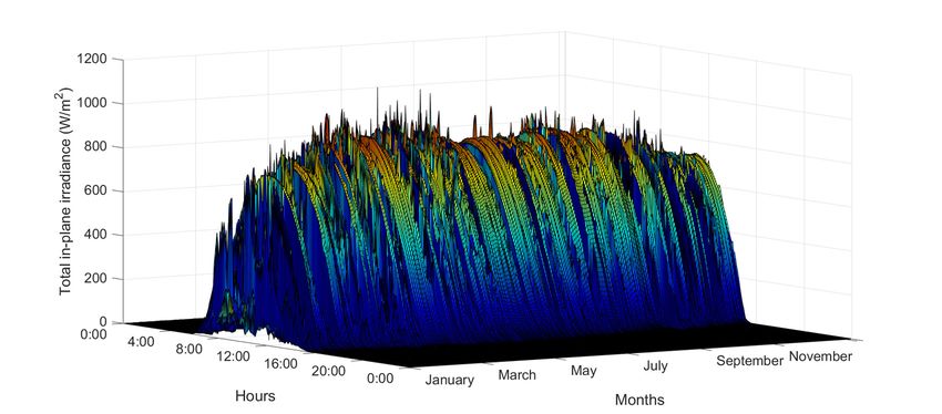
Figure 1 shows the total irradiance values received on the plane of the PV modules,
above, which
were were excluded from the classification process. In the colour map represen
recorded every 5 min during the entire period analysed in this work, from
Figure 1, it can
January 2011betoseen that2020.
February the There
maximumare two daily
periods,irradiance values
in 2012 and 2016, logically
where, due to occur
central failures
hours inofthe themonitoring system, no
day, between 12data records
p.m. andwere available,
4 p.m., andand which,
these as indicated
values are higher
above, were excluded from the classification process. In the colour map represented in
summerFiguremonths. It can also be seen how the irradiance values decrease from the
1, it can be seen that the maximum daily irradiance values logically occur in the
mum values
central in theofcentral
hours the day,hours
between of 12
thep.m.
day, towards
and thethese
4 p.m., and hours of sunrise
values are higher andin sunse
the summer months. It can also be seen how the irradiance values
obviously zero irradiance in the night hours. The greater number of hours of suns decrease from the
maximum values in the central hours of the day, towards the hours of sunrise and sunset,
the summer months in the geographical location where the measurements were ta
with obviously zero irradiance in the night hours. The greater number of hours of sunshine
evident.inItthecan also months
summer be observed how, onlocation
in the geographical days with
wherepassing clouds,were
the measurements there are
taken is variat
fluctuations
evident. inItthe irradiance
can also be observed values
how, onthroughout partclouds,
days with passing or allthere
the are
day. The daily
variations or irra
fluctuations in the irradiance values throughout part or all the day. The daily irradiance
profilesprofiles
with non-zero values shown in this figure are therefore those that were u
with non-zero values shown in this figure are therefore those that were used for
the classification carried
the classification out
carried outin
in this work.
this work.
Figure 1. Instantaneous in-plane irradiance values registered from 2011 to 2020 with a frequency sample of 5 min.
Figure 1. Instantaneous in-plane irradiance values registered from 2011 to 2020 with a frequency sample of 5 min.
Figure 2 shows a histogram in which the total daily irradiance values for each of the
Figure 2 shows
days shown a histogram
in Figure in which
1 can be observed. the
It can be total daily
seen that, irradiance
influenced by thevalues for each
greater or
lesser number of daily hours of sunshine throughout the year, and by the meteorological
days shown in Figure 1 can be observed. It can be seen that, influenced by the gre
conditions, the total daily irradiance received by the panels in the geographical location
lesser number ofthis
analysed in daily
workhours
can varyoffrom
sunshine
values ofthroughout the year,
less than 10 to values greaterand
thanby the meteoro
80 kW/m 2
conditions, theThe
per day. total
red daily
dashedirradiance received
lines show the values of bytotalthe panels
daily in the
irradiance geographical
received by the lo
panels that were obtained by the k-means algorithm to classify the analysed days in the
analysed in this work can vary from values of less than 10 to values greater than 80
three types named low (L), medium (M) and high (H).Appl. Sci. 2021, 11, x FOR PEER REVIEW 10 of 29
per day. The red dashed lines show the values of total daily irradiance received by the
panels that were obtained by the k-means algorithm to classify the analysed days in the
per day.
three Thenamed
types red dashed lines
low (L), show the
medium (M) values of total
and high (H). daily irradiance received by the
Appl. Sci. 2021, 11, 5230 panels that were obtained by the k-means algorithm to classify the analysed days in28the
10 of
three types named low (L), medium (M) and high (H).
Figure 2. Histogram corresponding to the daily total values of irradiance recorded on the plane of
the PV modules during the period 2011–2020.
Figure
Figure2.2.Histogram
Histogramcorresponding
correspondingtoto the
the daily total
total values
valuesof
ofirradiance
irradiancerecorded
recorded
onon
thethe plane
plane of of
thethe Figure
PVPVmodules
modules3 during
shows, forperiod
duringthe
the each 2011–2020.
period of the days of the period analysed, the average daily effi-
2011–2020.
ciency values of the set of 36 PV modules studied, connected to the same inverter, and
Figure3as
Figure
organised, 3shows,
shows,
mentionedfor
for each
each ofofthe
above, thedays
days
into of the
three period
of the analysed,
period
parallel the
analysed,
strings, eachaverage
the
with daily
average efficiency
daily effi-
12 modules con-
values
ciency of the set of 36 PV modules studied, connected to the same inverter, and organised,
nectedvalues of the
in series. Theset of 36 PVvalues
efficiency modulesof thestudied,
modules connected to the
represented in same inverter,
this figure wereandob-
as mentioned above, into three parallel strings, each with 12 modules connected in series.
organised,
tained by as mentioned
averaging above,
for each day into
thethree parallel
efficiency strings,
values (ηG) each with 12by
determined modules
Equation con-(3),
The efficiency values of the modules represented in this figure were obtained by averaging
nected
which in series.
were The efficiency
calculated every 5values
min. Itofcan
the be
modules represented
seen that, in this
for the days figure
with were ob-
the irradiance
for each day the efficiency values (η G ) determined by Equation (3), which were calculated
tained byshown
profiles averaging
in for each
Figure 1, day
the the
set of efficiency
panels values
worked on (ηaverage
G) determined
with by Equation
efficiencies (3),
ranging
every 5 min. It can be seen that, for the days with the irradiance profiles shown in Figure 1,
which
from were
around
the set calculated
8% worked
of panels to valuesevery
onof 5 min.
over 15%,
average It can
withso be seen that,
that this daily
efficiencies rangingfor the days
operating with
parameter
from around the irradiance
of the of
8% to values mod-
profiles
ules
overcan shown
15%, in variations
present
so that Figure 1, the
this daily set to
of up
operatingof8%.
panels worked
parameter of theonmodules
averagecanwith efficiencies
present ranging
variations of
from around
up to 8%. 8% to values of over 15%, so that this daily operating parameter of the mod-
ules can present variations of up to 8%.
Histogram corresponding
Figure3.3.Histogram
Figure corresponding to
tothe
thedaily
dailyaverage
averageefficiency values
efficiency of PV
values modules
of PV during
modules the the
during
period
period2011–2020.
2011–2020.
Figure 3. Histogram corresponding to the daily average efficiency values of PV modules during the
With regard
periodWith regard to
2011–2020. tothe
theoperation
operationof of
thethe
inverter, the daily
inverter, average
the daily efficiency
average values values
efficiency for the for
period of days analysed are shown in the histogram in Figure 4. The efficiency values of the
the period of days analysed are shown in the histogram in Figure 4. The efficiency values
inverter represented in this figure were obtained by averaging for each day the efficiency
With
of the regardrepresented
inverter to the operation offigure
in this the inverter, the dailyby
were obtained average efficiency
averaging values
for each dayfor
the
values (η inv ) determined by Equation (6), which were calculated every 5 min. It can be
the period of
efficiency days (η
values analysed are shown
inv) determined in the histogram
by Equation in Figure
(6), which 4. The efficiency
were calculated every 5values
min. It
seen that, in this case, the inverter under study can operate with an efficiency ranging
of the inverter represented in this figure were obtained by averaging for each day the
from values of around 75% to values close to 95%, although the values with the highest
efficiency
incidencevalues (ηinv) determined
were above by Equation
90%. The European (6), which
weighted were calculated
performance every 5given
of the inverter, min. It
by its manufacturers, is 95.1%, and 96% is the maximum efficiency, as reflected in Table 2.
These values were not reached in Figure 4, since the daily average values of this parametercan be seen that, in this case, the inverter under study can operate with an efficiency rang-
ing
canfrom
be seenvalues
that,ofinaround 75%
this case, toinverter
the values close to study
under 95%, although
can operatethe with
values
anwith the highest
efficiency rang-
incidence were above
ing from values of around90%.75%Theto European weighted
values close to 95%,performance
although theofvalues
the inverter,
with the given by
highest
Appl. Sci. 2021, 11, 5230
its manufacturers, is 95.1%, and 96% is the maximum efficiency,
incidence were above 90%. The European weighted performance of the inverter, givenas reflected in Table 2.
11 of 28by
These values were not
its manufacturers, reached
is 95.1%, andin Figure
96% is 4, since
the the dailyefficiency,
maximum average values of this parameter
as reflected in Table 2.
are shown.
These values However,
were not efficiency
reached invalues
Figure below
4, since90% indicate
the daily that the
average inverter
values of thisisparameter
working
below its proper operating state.
are shown. However, efficiency values below 90% indicate that the inverter is working
are shown.
below However,
its proper operating efficiency
state. values below 90% indicate that the inverter is working
below its proper operating state.
Figure 4. Histogram of daily average values of inverter efficiency over the period 2011–2020.
Figure 4. 4.
Figure Histogram
Histogramofofdaily
dailyaverage
averagevalues
values of inverter
inverter efficiency
efficiencyover
overthe
theperiod
period 2011–2020.
2011–2020.
And in the case of the so-called performance ratio (PR) (Equation (8)), the daily aver-
age values
AndAndinfor
inthe
the
the case of the
period
case of theanalysed
so-called performance
so-calledare shown inratio
performance the (PR) (Equation
histogram
ratio (PR) (8)),(8)),
in Figure
(Equation the5.daily average
It can
the be aver-
daily seen
values
that for the period analysed are shown in the histogram in Figure 5.
age values for the period analysed are shown in the histogram in Figure 5. It can be data
it varies between values above 0.3 and values very close to 1, It can
although be seen
for thethat
seen
setit varies between thevalues above 0.3 and values very close to 1, although for therange data set
thatrepresented,
it varies between daily average
values above PR values
0.3 that
and values determine
very close the
tointerquartile
1, although for the(Q1– data
represented, the daily average PR values that determine the interquartile range (Q1–Q3)
Q3) are 0.79 and 0.87,
set represented, and 0.83
the daily is the
average PRmedian
valuesof those
that data. the interquartile range (Q1–
determine
are 0.79 and 0.87, and 0.83 is the median of those data.
Q3) are 0.79 and 0.87, and 0.83 is the median of those data.
Figure 5. Histogram
Figure corresponding
5. Histogram correspondingtotothe
thedaily
daily average values of
average values ofthe
theperformance
performanceratio
ratio (PR)
(PR) forfor
thethe
inverter
Figure 5.together
inverter with
together
Histogram the
with theassociatedtomodules
associated
corresponding the dailyover
modules over the period
average period 2011–2020.
values2011–2020.
of the performance ratio (PR) for the
inverter together with the associated modules over the period 2011–2020.
It can
It can bebe seen,
seen, then,
then, that
that onceoncethethe adopted
adopted configurationofofthe
configuration themodules
modulesand andthethein-
inverter associated
verterItassociated
can be seen, with with
them
then, them is
thatis once fixed
fixedthe by the
by adopted design
the design and dimensioning
and dimensioning
configuration of the
of the set,
of the modules set,
and their
their
theop-
in-
operation presents margins of variation, whichshows
showshow
eration
verter presents
associated margins
with them of is
variation,
fixed bywhich
the design andhow these components
these components
dimensioning respond
theirtoop-
respond
of the set, to
changes
changes in in the
the meteorologicalconditions.
meteorological conditions.In In this
this way,
way, the
the energy
energy production
production will
willnot
notbebe
eration presents margins of variation, which shows how these components respond to
exclusively proportional to the irradiance received, but the variation in the meteorological
exclusively
changes in proportional to the irradiance
the meteorological conditions.received, but the
In this way, thevariation in the meteorological
energy production will not be
conditions affects the operation performance of the PV installation components, which can
exclusively proportional to the irradiance
lead to a variation in the expected production. received, but the variation in the meteorological
With respect to the first classification carried out in this work, obtained by applying
the k-means algorithm to all the total daily irradiance values of the 3237 days studied, the
results obtained are shown in Figure 6, where the number of days obtained in each ofconditions affects the operation performance of the PV installation components, which
Appl. Sci. 2021, 11, 5230
can lead to a variation in the expected production. 12 of 28
With respect to the first classification carried out in this work, obtained by applying
the k-means algorithm to all the total daily irradiance values of the 3237 days studied, the
results obtained are shown in Figure 6, where the number of days obtained in each of the
the
threethree types
types is represented,
is represented, as well
as well as the
as the values
values of the
of the totaltotal
dailydaily in-plane
in-plane irradiance
irradiance re-
received
ceived in in thethe modules
modules forfor
eacheachof ofthesethese days.
days. Of the
Of the totaltotal number
number of days
of days analysed,
analysed, 550
550
daysdays
werewere obtained
obtained belongingbelongingto theto lowthetype
low(which
type (which represents
represents 17.0% of17.0% of the
the total total
number
number of days analysed), 1043 corresponded to the medium
of days analysed), 1043 corresponded to the medium category (which represents 32.2%), category (which represents
32.2%),
and 1644 and 1644 corresponded
corresponded to the high to the high category
category (which represents
(which represents 50.8%).
50.8%). The totalThe
dailytotal
ir-
daily irradiance received 2
radiance received on theon the modules
modules on L on L days
days was was between
between 2.5 2.5
andand 35.8
35.8 kW/m
kW/m , with
2, with an
an average value of 21.3 kW/m 2 . For M days it was between 35.8 and 61.2 kW/m2 , with
average value of 21.3 kW/m 2. For M days it was between 35.8 and 61.2 kW/m2, with an
an average value of 50.4 kW/m 2 , and for H days, the range of the total daily irradiance
average value of 50.4 kW/m , and for H days, the range of the total daily irradiance values
2
values 2 , with an average value of 72.1 kW/m2 . This
varied varied
between between
61.2 and 61.2 and
81.9 81.9 2kW/m
kW/m , with an average value of 72.1 kW/m2. This implies
implies that on L days, the total in-plane
that on L days, the total in-plane irradiation received irradiation received
by theby PVthe PV panels
panels was between
was between 0.2 y
0.2 y 3.0 kWh/m 2 (an average value of 1.8 kWh/m2 ); between 3.0 and 5.1 kWh/m2 (an
3.0 kWh/m2 (an average value of 1.8 kWh/m 2); between 3.0 and 5.1 kWh/m2 (an average
2 ) on M days; and between 5.1 and 6.8 kWh/m2 (an average
average
value of value
4.2 kWh/mof 4.2 2kWh/m
)2 on M days; and between 5.1 and 6.8 kWh/m2 (an average value of
value of 6.0 kWh/m ) on H days.
6.0 kWh/m ) on H days. Of the total irradiance
2 Of the totalorirradiance
irradiationor irradiation
received by thereceived by the
panels during
panels during the nine years of monitoring considered in this
the nine years of monitoring considered in this work, 6.4% would have been received work, 6.4% would have been
on
received on L days, 29.2% would have been received on M days, and 64.4% would have
L days, 29.2% would have been received on M days, and 64.4% would have been received
been received on H days.
on H days.
Resultsof
Figure 6. Results ofthe
thefirst
firstclassification
classification
of of
thethe days
days according
according tototal
to the the total
dailydaily irradiance
irradiance value
value using
using the k-means algorithm.
the k-means algorithm.
Once this
thisfirst
firstclassification was
classification wascarried out,out,
carried the the
second classification
second was applied,
classification from
was applied,
which a totalaof
from which nineoftypes
total nine of daysofor
types clusters
days were obtained,
or clusters with different
were obtained, characteristics
with different charac-
from onefrom
teristics to another,
one to in terms of
another, inthe amount
terms of theof amount
irradianceof and its variation
irradiance and itsorvariation
fluctuation or
throughout the day.
fluctuation throughout the day.
A sample of the daily irradiance profiles obtained in each of the nine different different types
types
of days or clusters is shown in Figure Figure 7.7. The centroids corresponding to each of the the nine
nine
clusters obtained are
clusters obtained are shown
shownin inFigure
Figure8.8.InInaddition,
addition, the
the values
values of of total
total in-plane
in-plane daily
daily ir-
irradiance,
radiance, for each of the days obtained in each of the nine subcategories, are shown in
for each of the days obtained in each of the nine subcategories, are shown in
Figure
Figure 9,9, where
where the the number
number of of days
days obtained
obtained in in each
each one
one is
is also
also shown
shown on on x-axes.
x-axes. The
The
mean values of
mean values oftotal
totaldaily
dailyirradiance
irradiance forfor days
days H1,H1,H2H2
andand H3 were,
H3 were, respectively,
respectively, 72.4,72.4,
72.0
72.0 and 67.8 kW/m 2
and 67.8 kW/m 2. The .corresponding
The correspondingvalues values for days
for days M1, M2M1,andM2 M3andwere
M3 were
51.5,51.5,
48.5 48.5
and
and 2 and those of days L1, L2 and L3 were of 12.9, 25.6 and 27.9 kW/m2 ,
47.8 47.8
kW/m kW/m
2, and ,those of days L1, L2 and L3 were of 12.9, 25.6 and 27.9 kW/m2, respec-
respectively.
tively. In the In theofcase
case of L days,
L days, there there
was awas a larger
larger variation
variation in theinaverage
the average
valuevalue
of theoftotal
the
total daily irradiance value from L1 to L2 and L3 days. However, in the case of M days the
average total daily irradiance values presented by the three groups were similar to each
other, slightly higher on days with smaller fluctuations, and lower when there are more
fluctuations; the same behaviour was found for H days. It was observed that the days
within the three L-type categories, which are those with the lowest irradiance values, corre-Appl. Sci. 2021, 11, x FOR PEER REVIEW 13 of 29
daily irradiance value from L1 to L2 and L3 days. However, in the case of M days the
Appl. Sci. 2021, 11, 5230 average total daily irradiance values presented by the three groups were similar13 toofeach
28
other, slightly higher on days with smaller fluctuations, and lower when there are more
fluctuations; the same behaviour was found for H days. It was observed that the days
within the three L-type categories, which are those with the lowest irradiance values, cor-
sponded
respondedto days with
to days passing
with clouds.
passing There
clouds. were
There hardly
were any
hardly days
any dayswith
withdaily
dailyirradiance
irradiance
values in the range belonging to L days that corresponded to clear sky days, so
values in the range belonging to L days that corresponded to clear sky days, so that that inin
allall
three types, including L1, the passage of clouds and, therefore, fluctuations of irradiance
three types, including L1, the passage of clouds and, therefore, fluctuations of irradiance
values,
values,were
werethe
themost
mostfrequent
frequentsituation, resulting
situation, inin
resulting these low
these lowdaily irradiance
daily irradiancevalues.
values.
Appl. Sci. 2021, 11, x FOR PEER REVIEW 14 of 29
Figure 7. Sample
Figure 7. Sample of
of daily
daily irradiance
irradiance profiles
profiles obtained
obtained in
in the
the clusters
clusters L1,
L1, L2,
L2, L3,
L3, M1,
M1, M2,
M2, M3,
M3, H1,
H1, H2
H2
and H3.
H3.Appl. Sci. 2021, 11, 5230 14 of 28
Figure 7. Sample of daily irradiance profiles obtained in the clusters L1, L2, L3, M1, M2, M3, H1, H2
and H3.
Appl. Sci. 2021, 11, x FOR PEER REVIEW 15 of 29
Figure8.8.Centroids
Figure Centroidsof of
thethe
daily irradiance
daily profiles
irradiance obtained
profiles in the
obtained in clusters L1, L2,
the clusters L1,L3,
L2,M1,
L3,M2,
M1,M3,
M2, M3,
H1, H2 and H3.
H1, H2 and H3.Appl. Sci. 2021, 11, 5230 15 of 28
Figure 8. Centroids of the daily irradiance profiles obtained in the clusters L1, L2, L3, M1, M2, M
H1, H2 and H3.
Appl. Sci. 2021, 11, x FOR PEER REVIEW 16 of 2
Figure9.9.Total
Figure Totalin-plane daily
in-plane irradiance
daily and number
irradiance of days
and number ofobtained in the clusters
days obtained L1, L2, L3,
in the clusters L1,M1,
L2, L3, M1
M2, M3, H1, H2 and
M2, M3, H1, H2 and H3.H3.
With respect to the type M or days with medium values of the total daily irradiance
the days with smaller fluctuations due to the lower cloud passage are within the M1 sub
group. In addition, in this M1 group, some clear sky days were obtained, which corre
sponded to the irradiance received by the panels in January and December, winter day
in this geographical location, with a lower number of hours of sunshine than during th
rest of the year, which, despite being clear sky, give rise to values of total daily irradiancAppl. Sci. 2021, 11, 5230 16 of 28
With respect to the type M or days with medium values of the total daily irradiance, the
days with smaller fluctuations due to the lower cloud passage are within the M1 subgroup.
In addition, in this M1 group, some clear sky days were obtained, which corresponded
to the irradiance received by the panels in January and December, winter days in this
geographical location, with a lower number of hours of sunshine than during the rest of the
year, which, despite being clear sky, give rise to values of total daily irradiance in the range
of the named medium days. In the M2 and M3 categories, as a result of the classification,
the medium days which presented greater fluctuations in the irradiance values throughout
the day, due to the passage of clouds, logically obtained the highest fluctuations in the
M3 cluster.
Within the H clusters, with higher values of total daily irradiance, the days that
the algorithm considered to be within the H1 cluster corresponded to clear sky days
or days with less cloud passage, with fluctuations increasing on H2 type days, and to
a greater extent on H3 type days. The type of day with the highest incidence in this
geographical location corresponded to H1 days, which account for 40.2% of the total of
3237 days analysed.
Comparing M days with H days, it can be seen in Figure 7 how, in the irradiance
profiles of H days, the daily sunshine hours were somewhat higher (with sunset taking
place later and sunrise taking place before) than those of M days. Furthermore, it can also
be seen that, in the irradiance profiles of M days, the passage of clouds resulted in lower
irradiance values than in the fluctuations due to the passage of clouds on H days, with
these values being even lower in the profiles of L days. Thus, it can be considered that the
k-means algorithm correctly carried out the classification of the daily irradiance profiles
according to the total daily irradiance values and the fluctuations of the daily irradiance
throughout the day. The applied technique can be considered to be robust and easy to
apply [24,25].
Once the classifications were made, the performance of the PV system elements was
determined for each of the days obtained in the nine clusters. The results obtained for the
Appl. Sci. 2021, 11, x FOR PEER REVIEW 17 of 29
average daily PR value, corresponding to the operation of all modules together with the
inverter, are shown in Figure 10.
FigureFigure 10. Average
10. Average daily
daily performanceratio
performance ratio(PR)
(PR) of
of the
theset
setofof2626
PVPV
modules together
modules with with
together the inverter in the clusters
the inverter L1, L2, L1,
in the clusters
L3, M1, M2, M3, H1, H2 and
L2, L3, M1, M2, M3, H1, H2 and H3. H3.
It can be seen that there is a relationship between the type of day and the performance
with which the set of panels and the inverter works, ranging from mean values slightly
below 0.75 for L1 days, which are those with the lowest performance, to mean values close
to 0.9 for H2 days, which are the types of days on which there is a higher average PRAppl. Sci. 2021, 11, 5230 17 of 28
It can be seen that there is a relationship between the type of day and the performance
with which the set of panels and the inverter works, ranging from mean values slightly
below 0.75 for L1 days, which are those with the lowest performance, to mean values close
to 0.9 for H2 days, which are the types of days on which there is a higher average PR
value. The greatest dispersion of PR values within the different groups occurs on L1 days,
indicating that a greater heterogeneity of the days selected by the algorithm was obtained
within this group.
With regard to the behaviour of the set of modules and inverter, it can be observed
that on H days, the performance of their operation was similar on the three types of days,
regardless of the irradiance fluctuations that occurred. Within the M days, the performance
of M3 and M2 days were similar to each other, despite the differences in the fluctuations
of the daily irradiance profiles in these two groups, and both were slightly higher than
the performance of M1 days. The same was true for L days, in which the PR values of the
L2 and L3 days were similar to each other, and higher than those of the L1 days, which
corresponded to lower irradiance values.
It is noteworthy that H1 and M1 are not the days with the best average PR within
the categories of H and M days respectively, but it was found that days with passing
clouds, and therefore with fluctuations in production, had better average performance ratio
than clear sky days or days with fewer transitions. To see the reason for this behaviour,
Appl. Sci. 2021, 11, x FOR PEER REVIEW 18 of 29
Figure 11 shows the average daily efficiency of the PV modules obtained for the days on
each group.
Figure
Figure 11. Average
11. Average daily
daily efficiencyofofPV
efficiency PVmodules
modules in
inthe
theclusters
clustersL1,
L1,L2,L2,
L3,L3,
M1,M1,
M2,M2,
M3, M3,
H1, H2
H1,and
H2H3.
and H3.
Figure 11 shows that, although the production of energy in the modules is proportional
Figure 11 shows that, although the production of energy in the modules is propor-
to the irradiance received by them, the efficiency with which the modules transform solar
tional to theinto
radiation irradiance received
electricity variedby them, theon
depending efficiency
the type with
of day,which
suchthe modules
that, transform
on L1 days,
solar radiation
modules intowith
worked electricity varied
an average depending
efficiency on the
of 12%, andtype
on H2 of day,
days,such
which that,
areon L1 days,
those
modules
with theworked with an
best average average
efficiency of efficiency
the panels,of 12%,
had and on
average H2 days,
values which
close to 14%. are those
It can be with
theobserved
best average
that inefficiency of the
this H2 group, panels,
there haddispersion
was less average values close to
of the average 14%. It of
efficiency canthebe ob-
module
served from
that in one
thisday
H2togroup,
anotherthere
within the less
was samedispersion
group. It canofbethe
seen that, in efficiency
average general, theof the
days with
module from theone
lowest
daymodule efficiency
to another corresponded
within to L days.
the same group. It Within
can be the subcategories,
seen that, in general,
the efficiency improved from L1 to L2 and L3, as the total daily irradiance
the days with the lowest module efficiency corresponded to L days. Within the increased. Within
subcate-
these types of days, the variability or dispersion of the results within the same group was
gories, the efficiency improved from L1 to L2 and L3, as the total daily irradiance in-
creased. Within these types of days, the variability or dispersion of the results within the
same group was greater, which indicates, as already mentioned, the heterogeneity of pat-
terns that may exist within these subcategories. The behaviour of the efficiency of the PV
modules improved for days with medium irradiance. However, it is worth noting thatYou can also read