Climate, Agriculture and Food
←
→
Page content transcription
If your browser does not render page correctly, please read the page content below
Climate, Agriculture and Food
                                                         Submitted as a chapter to the Handbook of Agricultural Economics
arXiv:2105.12044v1 [econ.GN] 25 May 2021

                                                                                   Ariel Ortiz-Bobea†∗

                                                                                          May 2021

                                                                                          Abstract

                                                     Agriculture is arguably the most climate-sensitive sector of the economy. Grow-
                                                  ing concerns about anthropogenic climate change have increased research interest in
                                                  assessing its potential impact on the sector and in identifying policies and adaptation
                                                  strategies to help the sector cope with a changing climate. This chapter provides an
                                                  overview of recent advancements in the analysis of climate change impacts and adapta-
                                                  tion in agriculture with an emphasis on methods. The chapter provides an overview of
                                                  recent research efforts addressing key conceptual and empirical challenges. The chapter
                                                  also discusses practical matters about conducting research in this area and provides re-
                                                  producible R code to perform common tasks of data preparation and model estimation
                                                  in this literature. The chapter provides a hands-on introduction to new researchers in
                                                  this area.

                                           Keywords: climate change; impacts; adaptation; agriculture.
                                           Approximate length: 31,200 words.

                                              ∗
                                                 Associate Professor, Charles H. Dyson School of Applied Economics and Management, Cornell Univer-
                                           sity. Email: ao332@cornell.edu.
                                               †
                                                 I am thankful for useful comments provided by the editors Christopher Barrett and David Just as well
                                           as by Thomas Hertel and Christophe Gouel. Code and data necessary to reproduce the figures and analysis
                                           discussed in the chapter are available in a permanent repository at the Cornell Institute for Social and
                                           Economic Research (CISER): https://doi.org/10.6077/fb1a-c376.

                                                                                               1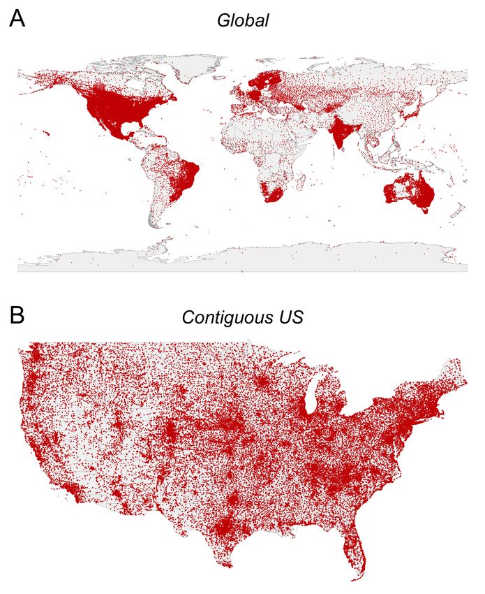
Contents
1 Introduction                                                                                                                                     3

2 Basic concepts and data                                                                                                                          6
  2.1 Weather and climate . . . .     .   .   .   .   .   .   .   .   .   .   .   .   .   .   .   .   .   .   .   .   .   .   .   .   .   .   .    7
  2.2 Adaptation . . . . . . . . .    .   .   .   .   .   .   .   .   .   .   .   .   .   .   .   .   .   .   .   .   .   .   .   .   .   .   .    8
  2.3 Weather data . . . . . . . .    .   .   .   .   .   .   .   .   .   .   .   .   .   .   .   .   .   .   .   .   .   .   .   .   .   .   .    9
  2.4 Climate models . . . . . . .    .   .   .   .   .   .   .   .   .   .   .   .   .   .   .   .   .   .   .   .   .   .   .   .   .   .   .   15
  2.5 Degree-days and agriculture     .   .   .   .   .   .   .   .   .   .   .   .   .   .   .   .   .   .   .   .   .   .   .   .   .   .   .   16

3 Climate change impacts and adaptation                                                                                                           19
  3.1 Biophysical approaches . . . . . . . . . . . . . .                          .   .   .   .   .   .   .   .   .   .   .   .   .   .   .   .   19
  3.2 The Ricardian approach . . . . . . . . . . . . .                            .   .   .   .   .   .   .   .   .   .   .   .   .   .   .   .   21
  3.3 Panel profit and productivity approaches . . . .                            .   .   .   .   .   .   .   .   .   .   .   .   .   .   .   .   24
  3.4 Statistical crop yield models . . . . . . . . . . .                         .   .   .   .   .   .   .   .   .   .   .   .   .   .   .   .   27
  3.5 Mixed statistical and biophysical approaches . .                            .   .   .   .   .   .   .   .   .   .   .   .   .   .   .   .   31
  3.6 Joint estimation of short and long run responses                            .   .   .   .   .   .   .   .   .   .   .   .   .   .   .   .   32
  3.7 Retrospective climate change impacts . . . . .                              .   .   .   .   .   .   .   .   .   .   .   .   .   .   .   .   35
  3.8 Statistical crop quality models . . . . . . . . . .                         .   .   .   .   .   .   .   .   .   .   .   .   .   .   .   .   36
  3.9 Modeling planting and harvesting decisions . . .                            .   .   .   .   .   .   .   .   .   .   .   .   .   .   .   .   37
  3.10 Irrigation and other input adjustments . . . . .                           .   .   .   .   .   .   .   .   .   .   .   .   .   .   .   .   40
  3.11 Market equilibrium and trade . . . . . . . . . .                           .   .   .   .   .   .   .   .   .   .   .   .   .   .   .   .   43
  3.12 Understudied problems and unsettled questions                              .   .   .   .   .   .   .   .   .   .   .   .   .   .   .   .   44

4 Coding and other empirical matters                                                                                                              46
  4.1 Aggregation of point weather data . . . . .                     .   .   .   .   .   .   .   .   .   .   .   .   .   .   .   .   .   .   .   47
  4.2 Aggregation of gridded weather data . . .                       .   .   .   .   .   .   .   .   .   .   .   .   .   .   .   .   .   .   .   52
  4.3 Estimating non-linear effects . . . . . . . .                   .   .   .   .   .   .   .   .   .   .   .   .   .   .   .   .   .   .   .   55
  4.4 Estimating within-season varying effects .                      .   .   .   .   .   .   .   .   .   .   .   .   .   .   .   .   .   .   .   65
  4.5 Spatial dependence . . . . . . . . . . . . .                    .   .   .   .   .   .   .   .   .   .   .   .   .   .   .   .   .   .   .   72
  4.6 Common robustness and sensitivity checks                        .   .   .   .   .   .   .   .   .   .   .   .   .   .   .   .   .   .   .   74

5 Conclusion                                                                                                                                      81

References                                                                                                                                        82

                                                      2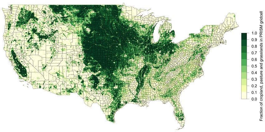
1    Introduction
Climate has always been critical to the development of agriculture. For instance, changes
in climate are believed to have played an imporant role in the origin of agriculture (Gupta,
2004; Matranga, 2017). More recently, the story surrounding the territorial expansion of
agriculture over the past few centuries was also one about adapting farming practices and
existing crops to new climates (e.g. Olmstead and Rhode, 2011).
    But climate is now changing at an unprecedented rate overwhelmingly due to human
causes (Pachauri et al., 2014). And even as the extent of global agricultural land stabilizes,
and agricultural productivity continues to rise, climatic shocks continue to play a central
role in explaining fluctuations in agricultural production (Lesk et al., 2016). In fact, recent
climate change appears to have already substantially slowed down global agricultural pro-
ductivity growth (Ortiz-Bobea et al., 2021). In this context, research is needed not only to
understand potential future impacts of anthropogenic climate change on agriculture, but also
to identify efficient strategies to enhance adaptation to a changing climate. This includes
identifying market failures and possible barriers to adaptation.
    Unlike mitigation of climate change, which requires a coordinated international effort
to reduce greenhouse emissions, adaption is generally framed as a local matter, something
that only local private agents have to deal with. However, farmers rely directly or indirectly
on public infrastructure, and buy technologies and sell products in markets with important
government presence and regulation. Moreover, the increasing globalization of agricultural
markets and technologies challenge this view. So agricultural adaptation to climate change
goes beyond the boundaries of the farm.
    This chapter is primarily aimed to introduce new researchers to the analysis of climate
change impacts on the agricultural sector. Most of the content should be highly accessible
but familiarity with matrix algebra is necessary to take fully advantage of the content. Im-
portantly, the chapter provides code and data to reproduce common tasks while conducting
research in this area, including data preparation and cleaning as well as the estimation of
semi-parametric models. All of the figures illustrating these techniques are fully reproducible
in R. R is a an increasingly popular open source statistical software that will ensure a wide
access to this material to all researchers.
    The chapter is organized in 3 main sections. Section 2 covers important basic concepts
and terminology regarding climate change and agriculture and discusses various aspects
regarding common datasets used in economic analysis in the field. Subsection 2.1 defines
weather as a random variable and climate as describing the moments of the underlying
distribution of that weather variable. Weather change and climate change mean different

                                              3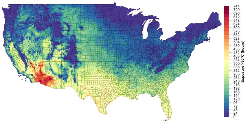
things and this clarification will allow a more precise discussion surrounding these concepts
throughout the chapter. Subsection 2.2 defines what we mean by adaptation to climate
change following the formal definition adopted by the Intergovernmental Panel of Climate
Change (IPCC).
     Conducting research in this area also require familiarity with different types of weather
data. Subsection 2.3 discusses important features about historical weather datasets including
their format (e.g. gridded, weather stations). I also provide the names of common datasets
used in the literature. Subsection 2.4 also discusses the basics of General Circulation Models
(GCM) and how the climate science community improves these models over time within
global inter-comparison projects that feed into the IPCC reports. Subsection 2.5 covers
some basic concepts regarding the use and interpretation of degree days. As it will become
apparent, temperature has been found to be a critical driver of agricultural production. The
use of degree days is not new in agriculture science, and I provide a historical perspective
on the concept and how its use has evolved in the more recent economic literature.
     Section 3 dives into specific areas of research or methodologies to assess the economic
impacts of extreme weather or climate change on agriculture. An important emphasis in
some of the techniques and approaches presented in this section deal with the extent to
which farmer adaptations are captured and represented. Subsection 3.1 provides an overview
of process-based biophysical approach of modeling crop yields and how these are integrated
into economic models to simulate climate change impacts to the agricultural sector. That
presentation provides an overview of the early literature as well as recent trends toward the
adoption of multi-model ensembles and inter-comparison projects.
     Subsection 3.2 transitions to discuss the cross-sectional Ricardian approach, one of the
first econometric approaches introduced to evaluate the impact of climate change on agri-
culture. Here I discuss some the advantages and pitfalls of this approach including recent
advances. The following subsection 3.3 deals with models estimating the effects of weather
fluctuations on agricultural profits or aggregate measures of productivity based on panel
data. Because these models include location fixed effects, they provide a more credible iden-
tification of the effect of weather than correctional approaches. I also provide an overview
of their limitations.
     Subsection 3.4 discusses the rise of statistical crop yield models in agricultural economics
and related fields. These models are also based on panel data but their focus on specific
crop yields allows researchers to engage in more detailed crop-specific treatment of weather
variables. I try to provide a historical perspective of the origin of these models before the
renewed interest in the context of climate change. I also briefly discuss new creative ways
to combine statistical and biophysical approaches to modeling crop yields in subsection 3.5.

                                               4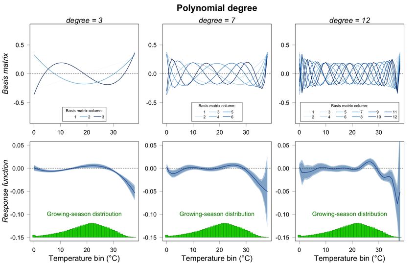
These new efforts provide exciting new frontiers of collaboration with natural scientists.
    In subsection 3.6 I discuss an emerging area of research proposing new methods to over-
come certain perceived limitations of both cross-sectional and panel approaches. I describe
these recent advances and their limitations. I highlight new work that clarifies the theoreti-
cal interpretation of panel estimates. I also provide a brief overview to retrospective climate
change studies in subsection 3.7. Most of the research emphasis has focused on assessing
future potential impacts of climate change on the sector. However, anthropogenic forces
have already changed climate which is about 1°C warmer than in pre-industrial times. As
climate continues to change, such retrospective studies are likely to increase in popularity. I
provide a brief overview of early and more recent studies. The rest of section 3 is less about
methods, and more about various aspects of capturing climate change impacts and farmer
and market responses.
    There is a vast literature assessing impacts on crop yields, but there is much less work
focusing on the impact on crop quality. Subsection 3.8 presents recent work on this topic and
lays out some challenges for future work. Subsection 3.9 discusses the analysis of planting
and harvesting decisions, ranging from the timing of planting, to the decision to increase
cropping frequency (e.g. double cropping). Naturally, irrigation is central to agriculture and
is often perceived as an important mechanism for farmers to adapt a water scarcity in a
changing climate. I cover this topic in subsection 3.10, where I discuss early studies but also
provide a look to more recent work based on new data sources collected from satellites or
providing high-frequency information about water use at the farm level. I also discuss the
role of trade in the analysis of climate change impacts on agriculture in subsection 3.11.
    I conclude section 3 addressing various questions that still seem unsettled and where
more research is likely needed (subsection 3.12). For instance, there is insufficient work on
the economic of agricultural innovation in the context of a changing climate. For instance, it
is unclear whether current levels and the current nature of agricultural R&D is adequate in
a rapidly changing climate. In addition, there are many lingering uncertainties regarding the
important of changing pest pressure as well as the rise of soil salinity in a warming world.
There is also little emphasis on climate justice.
    Section 4 provides more practical and hands-on guidance regarding common empirical
tasks in this area of research. The chapter is accompanied with reproducible R code that
illustrates how to perform many of these tasks in a systematic way. Providing the accompa-
nying code seems important for new researchers entering this field because many of the data
management and estimation techniques are yet not standard in agricultural economic cur-
ricula. The code provided can be easily adapted to new projects and accelerate the learning
curve of new entrants. For instance, the section provides an overview on how to efficiently

                                              5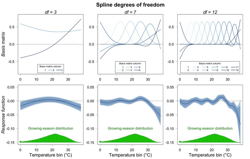
aggregate point and gridded weather datasets (subsections 4.1 and 4.2). The techniques that
I introduce are based on matrix algebra and sparse matrices to speed up aggregation relative
to standard “canned” functions in R packages.
    An important empirical consideration in the analysis of the effects of extreme weather and
climate change on agriculture is the presence of nonlinearities and thresholds. Climate change
will lead to more frequent extreme weather and thus capturing such nonlinearities is critical.
Importantly, temporal and spatial averaging of weather conditions can conceal exposure to
extreme weather and thus more advanced techniques are required to overcome such obstacles.
In subsection 4.3 I describe how to estimate non-linear effects of weather variables semi-
parametrically based on bins representing the entire distribution of time exposure to varying
environmental conditions (e.g. temperature). I also describe how to construct these datasets.
The R code provided illustrates not only how to construct these data but also how to estimate
these models. I also clarify certain misconceptions and confusion regarding the estimation
of these models. In subsection 4.4 I also present a two-dimensional generalization of the
semi-parametric model above that allows simultaneously for non-linear and within-season
varying effects. This is particularly valuable when trying to capture varying sensitivities to
environmental conditions within the growing season.
    A common feature of agricultural and climate data is spatial dependence, which generally
translates into spatial dependence in a regression setting. Subsection 4.5 introduces a few
approaches to deal with this by either correcting for spatial dependence or by harnessing
spatial dependence to obtain a more efficient estimator. Finally, subsection 4.6 discusses
common robustness checks in the literature as well as strategies to present these in a concise
manner in a “specification chart”. I also provide reproducible code to conduct these sensitivity
checks.
    I finally conclude in section 5 where I provide some final thoughts about the potential
for new collaborations and for enhancing the impact of economic research in this field.

2    Basic concepts and data
Here I discuss basic concepts and terminology regarding climate change and how farmers
respond to it. This preliminary step is critical in helping new researchers understand the
common language used in this field.

                                               6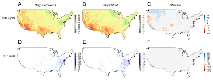
2.1    Weather and climate
Throughout this chapter I refer to “weather” and “climate” which are related but distinct
concepts. A useful way to characterize their relationship is to think about weather as a
random variable representing the state of the atmosphere. That random variable could
represent, say the “average temperature during the month July in Ithaca, NY”. The value
taken by this variable on a given year represents weather conditions.
    In contrast, “climate” refers to the moments of the probability distribution of that random
variable. Thus, quantities such as the “long term average” or the “inter-annual variability” of
this random variable relate to climate. It is often the case that climatologists (and economists
by extension) refer to “climatology” as the 30-year average of a weather variable, and as
“climate variability” as the inter-annual variance of a weather variable. This concept is
different from the term “intra-annual weather variability” which refers to the variability of
weather conditions between contiguous time periods within a season or the year.
    As a result, the term “climate change” refers to the change in the long term distribution
of weather conditions at a given location. By definition, it is a long term process because
climatologies are defined over several decades. It follows that climate change eventually
results in the rising frequency of weather events that were previously considered unusual or
extreme. That being said, because of natural variability in the climate system, a sequence of
extreme weather events is not evidence of climate change per se. Indeed, assessing changes
in climate requires a relatively long time series of weather observations.
    In addition, the term “climate change” should also not be conflated with “weather change”
which may refer to either inter-annual or intra-annual fluctuations in weather conditions
depending on the context. Moreover, recent weather trends should not be conflated with
climate change. There are well known cyclical components in the climate system such as El
Niño-Southern Oscillation (ENSO) which are linked to cyclical changes in weather patterns
in various parts of the world. These multi-year weather patterns do not constitute climate
change, though climate change may alter their intensity.
    Climate change can have both natural or human causes. An entire field in climate science
called “detection and attribution” focuses on determining whether observed historical changes
in climate can be attributed to specific causes. The term “anthropogenic climate change”
thus refers to changes in climate that have been shown to originate from human activities,
including through the emissions of greenhouse gases.
    Making the clear distinction between weather and climate is important. Not only does
it help avoid ambiguous terminology and helps convey ideas more clearly, but it also has
economic implications. The reason is that while economic agents cope directly with weather
conditions, they actually form expectations about climate.

                                               7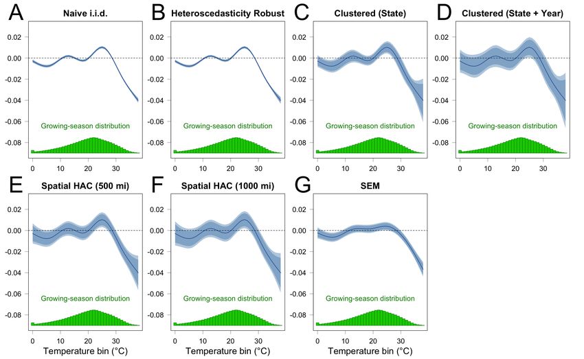
2.2    Adaptation
According to the IPCC (2014), adaptation to climate change in human systems is “the process
of adjustment to actual or expected climate and its effects, in order to moderate harm or
exploit beneficial opportunities”. It should be clear why assessing the potential impacts of
climate change on agriculture should require considering the degree to which farmers would
adapt a new climate. Not accounting for adaptation would naturally overstate potential
damages and under appreciate potential opportunities.
    Agricultural economists have mostly focused on adaptation undertaken by farmers. If
you consider weather as a stochastic essential input, then the adjustments of traditional
inputs under the control of the farmer to maximize profit or utility in response to weather
fluctuations are forms of farmer adaptation. Input decisions are typically sequential in na-
ture (Antle, 1983), so certain decisions are committed irreversibly early in the season (e.g.
crop and parcel choice, acreage, etc.) before the farmer gets to observe the weather realiza-
tion. As a result, some inputs remain fixed throughout the growing season, constraining the
farmer to a limited range of adaptations. In general, these short-run adaptations to weather
fluctuations understate the range of adaptations undertaken by farmers when considering
long run adjustments in response to a changing climate.
    However, certain short run adjustments may not be available to the farmer in the long
run. One example may be irrigation. For instance, a farmer with land equipped for irrigation
may increase the amount of water used in response to dryer weather conditions. However, if
the source of irrigation water is projected to be depleted or water prices are expected to be
much higher in the future, then adjustments made in the short run may not be indicative of
those available in the long run.
    The empirical characterization of future farmer adaptations generally relies on historical
behavior. But past behavior relative to a change in a weather shock (or small changes in
climate) could mischaracterize the degree to which farmers may adapt in the long run. This
is somewhat related to the Lucas critique applied to the climate change context (see Kahn,
2014).
    Accounting for adaptation is critical to the estimation of potential future climate change
impacts on agriculture. This has been a major emphasis in the literature. Not accounting for
adaptation would naturally overstate damages. Thus researchers typically seek to constrain
or characterize their findings depending on the degree to which farmers can adapt in their
modeling approach.
    Capturing or measuring long run adaptations to climate change is challenging. It ulti-
mately requires capturing adjustments to the production process in response to a long term
change in the distribution of weather conditions. Ideally, characterizing this process requires

                                              8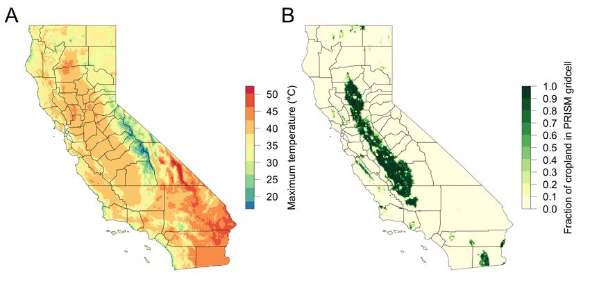
a long time series of weather and production decisions. Long longitudinal datasets with de-
tailed information about production practices are very rare, making detection of adaptation
activities elusive.
    Explicitly accounting or modeling all possible farmer adaptation to a changing climate
is intractable. Farmers have numerous potential adjustments to their production decisions.
This could include changes in input use, tilling practices, planting dates or crop mix for crop
production, or the change in management, feed, animal breeds, equipment or infrastructure
for livestock production. As a result, researchers often rely on indirect evidence to identify
or quantify adaptation (or lack of).
    The IPCC (2014) also employs the term “maladaptation” which refers to “actions that
may lead to increased risk of adverse climate-related outcomes, increased vulnerability to cli-
mate change, or diminished welfare, now or in the future”. However, this term is rarely used
in mainstream economic academic discussions. In the agricultural context, this would mean
that agriculture is growing more vulnerable to climate change, such as becoming increasingly
sensitive to higher temperature (e.g. Lobell et al. 2014; Ortiz-Bobea et al. 2018, 2020). How-
ever, such changes in sensitivity to extreme temperature may result from an optimal tradeoff
so referring to such phenomena as maladaptation which carries a undesirable connotation
may be misleading.
    Note that the notion of economic efficiency is absent from the IPCC characterization of
adaptation. Economists bring a unique perspective to analyze the economic desirability of
adaptive investments from a welfare perspective. This is more often than not absent for the
analysis and discussions surrounding adaptation.

2.3    Weather data
Weather data is a fundamental component of conducting empirical analysis of climate change
impacts and adaptation. Here I highlight some key features of such data without being
exhaustive. I encourage readers to consult Auffhammer et al. (2013) for a complete guide
on how to use weather data and climate model output in economic analysis.
    Basic weather variables like air temperature and precipitation are commonly measured
in weather stations. These are commonly (but not always) government-run facilities with
the necessary instrumentation to record information about atmospheric conditions. In these
facilities, temperature has historically been measured directly via thermometers, whereas
precipitation is measured via rain gauges, which measure the amount of precipitation falling
within a time interval, typically a day. In certain countries like the US and parts of Western
Europe, this instrumental record dates back to the 19th century. Air temperature varies

                                              9
throughout the day, and it is sometimes possible to obtain hourly data for certain regions in
recent years. But data is more commonly available at the daily, monthly or annual scales.
In such cases summary statistics are reported including maximum, average and minimum
temperature or total precipitation over the given time period. Note that strict rules and
protocols govern the recording and reporting of official weather data.
Temperature measurements prior to the use of thermometers are based on proxy variables
(e.g. tree rings) and are used to reconstruct past weather conditions in paleoclimatology.
Since the late 1970s, researchers can also obtain remotely-sensed temperature from satellites
which are derived indirectly from microwave radiation.
Because temperature and precipitation are commonly measured at specific locations
(weather stations) throughout the landscape, such type of weather data is referred to as
“point data” in Geographical Information Systems (GIS). A point is associated with precise
geographical coordinates and is thus said to be geo-referenced.
Figure 1A provides an overview of the spatial distribution of the more than 100,000
weather stations reporting daily information in the Global Historical Climatology Network
(GHCN) in 2020. The GHCN is the world’s largest database of climate summaries from land
surface stations across the globe and it is managed by the National Oceanic and Atmospheric
Administration (NOAA). The distribution of weather stations can be very sparse across the
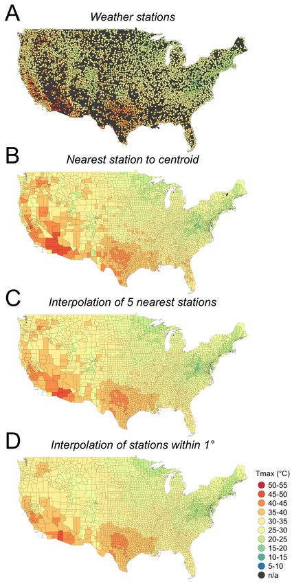
world, even within countries like the US (Fig. 1B). This spatial sparsity raises challenges
for obtaining correct weather information in areas located far from weather stations, partic-
ularly when the landscape has pronounced orography. In section 4.1 I provide a brief and
reproducible introduction on (very) basic weather station data interpolation.
With the goal of providing more complete spatial coverage in a consistent fashion, cli-
matologists have developed “gridded” weather datasets based on various interpolation tech-
niques. These interpolation techniques often rely on elevation and other physical factors that
are known to affect both temperature and precipitation. These procedures are considerably
more sophisticated than a simple spatial interpolation. These geo-referenced datasets come
on a regular grid and are referred to as “raster” data in GIS. They are characterized by
a spatial resolution, often measured in degrees or distance. Raster data is fundamentally
structured as a matrix, where each entry corresponds to a patch of of the Earth’s surface.
It is important to clarify that some of gridded weather datasets can sometimes incorporate
numerical weather models (similar to those used for weather forecasts). In that case these
gridded weather data are referred to as “reanalysis”. This is one example of “modeled”
data that incorporates both observations (from weather stations) and information from a
mechanistic weather simulation model. The advantage of such data is that they can provide
a spatially and temporally consistent field of weather information even when there are gaps
10Figure 1: Spatial distribution of weather stations in the Global Historical Climatology Net-
work in 2020.
11Spatial Temporal
Name Coverage Resolution Coverage Resolution Source
PRISM CONUS 4 km 1981 – daily Daly et al. (1997)
Daymet North America 1 km 1980 – daily Thornton et al. (2014)
NARR North America 0.3 deg 1979 – 3-hourly Mesinger et al. (2006)
NLDAS North America 0.125 deg 1979 – hourly Xia et al. (2012)
GLDAS Global 0.25 deg 1948 – 3-hourly Rodell et al. (2004)
GMFD Global 0.25 deg 1948 – 2016 daily Sheffield et al. (2006)
Table 1: Commonly used gridded weather datasets.
in the underlying weather station data. They can also provide output of variables that are
actually not being actually measured in any consistent way (e.g. temperature or wind speed
at high altitudes).
So far I have only discussed weather variables and data relating to atmospheric conditions.
For certain applications the researcher might be interested in more direct measures of water
content or temperature in the soil. Direct measurement of soil water content and temperature
are very rare and only available over limited areas and time periods in a handful of nations.
Obtaining data on these variables at larger scales generally requires relying on modeled data,
although new satellite sensors are increasingly able to indirectly measure some of these soil
moisture variables.
The evolution of soil water content and temperature is a complex process that is typically
modeled with a Land Surface Model (LSMs). An LSM takes “forcing” or exogenous variables
as inputs (e.g. surface temperature, precipitation, wind, air humidity, etc.) to characterize
the evolution of soil conditions over time. Some of the key variables of interest include soil
water content but also soil temperature. These models provide a modeled snapshot in time
of these variables at various depths in the soil, often down to a couple meters. The use of
certain highly detailed LSM datasets can be cumbersome as they may require manipulating
terabytes of data. For some applications, the use of simpler drought indices, such as the
Palmer Drought Severity Index (PDSI) or the Standardized Precipitation Index (SPI), may
suffice (see Heim, 2002). These indices seek to approximate water deficit conditions based
on water supply (precipitation) and demand (evapotranspiration and runoff) with relatively
simple algorithms.
In table 1 I include a list of commonly used gridded weather and land surface datasets
with at least a daily temporal resolution. This list is by no means exhaustive but provides
the reader with a starting point in their analysis. Monthly datasets are easier to come by
and typically offer longer temporal coverage. For instance, the widely used monthly version
of Oregon State University’s Parameter-elevation Regressions on Independent Slopes Model
12(PRISM) dataset over the contiguous United States (CONUS) is available since 1896.
An important point regarding empirical work in this literature is the common mismatch in
spatial resolution between agricultural and weather data. Agricultural data is often available
to researchers after being aggregated to administrative units such as counties, states or even
countries. This aggregation is sometimes performed from micro-data from surveys or census
to preserve anonymity of individual farmers. Unless a researcher is dealing with field or farm-
level data, the spatial resolution of agricultural data is typically coarser than that of gridded
weather data. That is, several grid cells fall within the boundaries of the administrative unit.
As a result, researchers end up aggregating the gridded weather data to the administrative
unit level.
This naturally raises the question of how should gridded weather data be aggregated to
administrative levels. Certain administrative units (e.g. US states) can be fairly large and
heterogeneous and contain areas with little to no agricultural activity (e.g. like high moun-
tains or deserts). In other words, weather conditions in certain parts of the administrative
unit may be irrelevant for agricultural production within that unit. A common practice is
to rely on fine scale land cover data (e.g. cropland, pastures, or a combination) to use as
an aggregation weight. Land cover data comes in raster format and with spatial resolutions
ranging anywhere from 30m to 1km depending on the region of the world.
To illustrate this point, Fig. 2A shows maximum temperature in California on August 16,
2020 when possibly the highest temperature ever recorded on Earth (54.4 °C) was measured
in the Death Valley (darkest shade of red). This daily gridded data is from PRISM and
shows wildly varying weather conditions across the state on the very same day. However,
agriculture is mostly concentrated in the Central Valley region. This can be seen in Fig.
2B showing the share of cropland within each PRISM grid cell. A common practice is to
aggregate the weather (panel A) variable within each county (or within the state) based on
weights proportional to the cropland cover (panel B). The large climatic variations within
California illustrate how critical land cover information can be for representing environmental
conditions within administrative units.
Intuitively, spatial weighting procedures should make little difference if we are located
in a relative small or homogeneous administrative units. However, potentially substantial
differences could arise between different weighting schemes in the presence of climatically
diverse units. Some have suggested that the weighting should be performed by value (rather
than land cover) although it seems unclear how livestock would be accounted for in such
circumstances. One way to think about issues about spatial aggregation is to frame it in
terms of measurement error. It turns out that implications of these practices have not
been chracterized. Researchers often end up showing regression results under alternative
13Notes: Panel A shows maximum temperature corresponding to August 16 of 2020 over California. This is
gridded daily data from PRISM. Panel B shows the share of cropland contained in each of the PRISM grid
cells. The grid cell share was derived from finer scale 30m land cover data for 2016 from the National Land
Cover Database (NLCD).
Figure 2: Gridded data and cropland land cover in California.
14weighting schemes to assuage concerns during the peer review process. This practice seems
suboptimal and more systematic analysis of the consequences of various strategies of spatial
data aggregation are needed.
There are also issues regarding temporal aggregation in weather data. Aggregating
weather data over time can also result in measurement error if the weather conditions are
non-additive and if non-linearities in exposure to various levels of weather conditions are
important, which they likely are.
2.4 Climate models
Climate scientists have developed Global Circulation Models (GCMs) to simulate the evolu-
tion of the climate system. These models are fundamentally similarly to numerical weather
models used in weather forecasting, but incorporate a more complete representation of en-
ergy exchanges between land, oceans, sea ice and the many layers of the atmosphere. Central
to these models are the Navier-Stokes equations, partial differential equations that describe
the movement of viscous fluids. Solving these equations to describe moving air masses in
three dimensions requires considerable computational power, which is why running these
models requires super computers. Major countries have research groups and labs with their
own version of these models.
In order to learn more about factors affecting our climate system, modeling groups have
joined a global inter-comparison project called the Coupled Model Inter-comparison Project
(CMIP). Four of such inter-comparisons have been completed (CMIP Phases 1, 2, 3 and 5)
and there is one under way (CMIP Phase 6 or CMIP6). The key feature of CMIP is the
parallel implementation of identical climate experiments across a wide range of GCMs. Some
of these experiments are designed to learn about specific aspects of these models, so that
GCMs can be improved. However, some of these climate experiments are much more policy
relevant and seek to understand how the global climate system is influenced by anthropogenic
influences.
Various experiments seem particularly policy relevant and are commonly used by economists.
Using CMIP6 terminology, these include the Shared Socioeconomic Pathways (SSPs, see Ri-
ahi et al., 2017), including SSP1-2.6, SSP2-2.5, SSP3-7.0 and SSP5-8.5. The SSPs correspond
to different scenarios about the nature economic development and the pathway of climate
forcing (e.g. emissions) throughout the century. The appended numbers to these scenarios
(i.e. 2.6, 4.5, 7.0 and 8.5) represent the additional radiative forcing on our climate system
in Watts/m2 in the year 2100. The higher the number, the higher the additional radiative
forcing, and the higher global temperatures are projected to rise. These scenarios are anal-
15ogous to the Representative Concentration Pathways (RCPs) scenarios used in CMIP5, and
the Special Report on Emissions Scenarios (SRES) used in CMIP3. Researchers can relate
these projected future states of the atmosphere under various GCMs and SSPs with the
“historical” experiment that seeks to replicate the conditions of our historical climate system
from the nineteen century through 2015 in the case of CMIP6. The “historical” experiment
considers both historical levels of both natural (e.g. volcanic eruptions from el El Chichón in
1982 and Pinatubo in 1991) and anthropogenic forcing (e.g. greenhouse gas emissions since
the industrial revolution).
Other relevant climate experiments that are relatively underused by economists are the
“historicalNat” in CMIP5 and “hist-nat” in CMIP6. These experiments run a historical sim-
ulation but only with natural forcing. That is, the output of these experiments provide a
counterfactual sequence of modeled weather trajectories that exclude human influence from
the climate system. In climate science, the comparison of these experiments and the “histor-
ical” experiment is a foundation of attribution studies that seek to establish to what extent
extreme weather events (e.g. heat waves) are likely to arise because of human influences,
and not because of natural variability. Some studies have used this approach to analyze the
historical impact of anthropogenic climate change on agriculture (See section 3.7).
It should be noted that output from climate models is gridded in nature (raster format)
and can be manipulated in the same way than gridded weather datasets previously discussed.
Finally, it is worth noting that the CMIPs serve as the basis of the Assessment Reports
(AR) for the first working group (WGI) of the Intergovernmental Panel of Climate Change
(IPCC) charged with describing the physical basis of the factors affecting our climate system.
In fact, the name of the CMIP and the AR are in phase, so that the lessons from CMIP6 feed
into the the Sixth Assessment Report of AR6. The ARs serve as an input for international
negotiations regarding adaptation and mitigation of anthropogenic climate change within
the United Nations Framework Convention on Climate Change (UNFCCC).
2.5 Degree-days and agriculture
A growing number of studies rely on variables representing “degree days”, “growing degree
days” (GDD), “damaging degree days” (DDD), “extreme degree days” (EDD) or “killing de-
gree days (KDD) for analyzing the effect of cumulative temperature exposure on agricultural
production. Although the growing popularity of degree-day measures seems relatively recent
in agricultural economic research, the concept has roots that are centuries-old (Réaumur,
1735). Here I provide a brief background on the concept and how to compute these variables.
A degree-day is one of the many units of measurement of thermal time. Thermal time is
16a physical quantity measured in units of temperature × time. This concept is very familiar
to scientists studying phenology, which is the study of how the periodicity of biological cycles
are influenced by their environment. The concept emerged as an heuristic tool to predict
the length of the different phases of plant life cycles (Réaumur, 1735). Some measures
of thermal time are highly correlated with the timing of numerous phenological events, or
cyclical natural phenomena, such as insect or plant development. In plants, such development
phases are typically signaled by the appearance of new and differentiated organs such as
the emergence of subsequent leafs and flowers or the formation of fruit. French scientist
René-Antoine Ferchault de Réaumur laid the foundations of thermal time in the eighteenth
century as recalled by Wang (1960): “He summed up the mean daily air temperatures for
91 days during the months of April, May and June in his locality and found the sum to be
a nearly constant value for the development of any plant from year to year.” Thermal time
subsequently became a pivotal concept in phenology (Hudson and Keatley, 2009, ch. 1).
Indeed, the timing of many biological cycles, particularly in plants and insects, is closely
correlated with thermal time accumulation. For this reason, biologists coined a term that
measures thermal time accumulation, Growing Degree-Days (GDD). This biological thermal
time corresponds to cumulative temperature during a period of time. Intuitively, it is an
amount of accumulated exposure to heat.1 This quantity is often defined mathematically. As
shown in equation 1, thermal time T is typically expressed as a function of two temperature
thresholds, h and h and two points in time, t0 and t1 .
ˆt1
h−h if h(t) > h
T (h, h, t0 , t1 ) = H(t)dt where H(t) = h(t) − h if h(t) ∈ ]h; h] (1)
t0
if h(t) 6 h
0
This definition implies that any measurement of thermal time is a function of the two
temperature thresholds and a duration. In fact, the two temperature thresholds, h and h,
are experimentally determined to yield a nearly linear relationship between thermal time
accumulation and biological development.2
The link between temperature and the timing of biological cycles can be explained at
1
Although strictly speaking this is inexact because “heat”, in thermodynamics, is a form of energy which is
measured in Joules, not in temperature units. There is, however, a direct relationship between temperature
change of a body and the heat it receives.
2
For instance, for the early-maturing dwarf hybrid sunflower plant (Pioneer 6150) with h defined as 0°C
(undefined h), the first two true leaves appear after exposure to 249-313 GDD, flowering begins at 935-1077
GDD, and maturity is achieved after 1780-1972 GDD.
17the molecular level within cells. Air temperature, at the most basic level, affects cellular
function, and animals and plants have developed strategies to take advantage of climatic
conditions conducive to their growth and largely avoid conditions that are harmful. In the
case of crops, when air temperature is below the lower threshold, h, also referred to as
the crop-specific “base temperature,” or above the higher threshold, h, crop development
essentially stops (Ritchie et al., 1991; McMaster and Wilhelm, 1997). Enzymes, which are
proteins that accelerate biochemical reactions within cells, become too rigid at low temper-
atures and coagulate at very high temperatures, leading to slow or entirely inhibited crop
growth (Bonhomme, 2000). In other words, because plants cannot regulate much their own
temperature, their metabolism is subject to outside temperature, which affects the speed of
biochemical reactions.3
This relationship is not perfectly linear because the timing of these development stages
are also dependent on adequate light, water, and nutrients in addition to appropriate temper-
ature. However, temperature remains the major factor explaining the timing of development
stages. This explains why agronomists and farmers use GDDs to estimate stages of crop
development and weed and pest life cycles.
Note that variables that measure the amount of time exposed to certain temperature
levels are closely related to the concept of degree days. Degree day are measures of cumulative
temperature exposure between two temperature thresholds. The concept is very general and
is used outside of agronomic sciences. For instance, engineers and energy analysts rely on
Cooling Degree Days (CDD) and Heating Degree Days (HDD) to predict energy consumption
for cooling in the summer, and for heating in the winter, respectively.
Possibly the oldest use of degree days was to predict phenology, the timing of life stages
in plants and certain animals (Réaumur, 1735). The modern incarnation of this concept
applied to plants is reflected in the modern use of Growing Degree-Days (GDD) which are
precisely reserved to predict crop stages (Bonhomme, 2000). Field crops are characterized by
their crop maturity rating which indicates the amount of “cumulative temperature” measured
in GDD to reach maturity. Short-season cultivars require less heat of the growing season
to reach maturity. For this reason such cultivars are used in colder climate in temperature
countries like the US, where the non-freezing period that is fatal to most crops is relatively
short. Thus, farmers choose a crop maturity rating based on their local climate.
The implication is that once farmers plant a given cultivar, unexpectedly warm or cold
conditions can accelerate or delay the timing to reach crop maturity and harvest. As a
result, changes in GDD can affect yield, because shortening the time the crop spends on
3
Organisms unable to actively regulate inner temperature to favorable levels are coined “ectotherms”.
This is not only the case of plants, but also of “cold blooded” animals such as insects, reptiles, etc.
18the field shortens the time the crop has to accumulate biomass. Similarly, lengthening the
timing the crop spends on the field can expose the crop to perilous conditions at the end
of the season (e.g. damaging Fall frost). However, the concept of GDD is not intended to
predict yield, but to predict phenology. Many economic studies rely on “GDD” measures to
predict yield. This is incorrect. A more rigorous use of the term that does not introduce
confusion with its agronomic use is to simply describe degree day variables in terms of the
range of temperature used to defined them, like “degree days 8-30°C”. Note that degree
days capturing exposure to relatively high thresholds, say 30°C, are commonly referred to
as Extreme Degree Days (EDD), Killing Degree Days (KDD) or Damaging Degrees Days
(DDD). Similarly, describing degree days by their threshold, such as “degree days over 30°C”
seems generally more appropriate.
3 Climate change impacts and adaptation
This section provides an overview of the main research questions and the methods used
to evaluate climate change impacts and adaptation in the agricultural sector. While the
discussion will cover developments over the past 2 decades, I put some emphasis on the
evolution of the literature as well as recent contributions. I also spend some time discussing
unresolved or relatively unexplored research questions. I also invite the reader to consult
several overview articles on methods of assessing climate change impacts on agriculture and
other sectors, including Blanc and Schlenker (2017), Carter et al. (2018) and Kolstad and
Moore (2020), to name just a few.
3.1 Biophysical approaches
Most of the early work assessing climate change impacts on agriculture is fundamentally
based on biophysical models (e.g. Adams 1989; Adams et al. 1990; Rosenzweig and Parry
1994). These plant science models mechanistically characterize the effect of environmental
conditions (e.g. sunlight, water availability, air and soil temperature, carbon dioxide concen-
trations, air humidity, etc.) on the physiological processes that underly crop yield formation.
This type of approach typically assume farmers adopt a series of more or less sophisticated
management practices including choice of cultivar, fertilization decisions, planting time, etc.
These models are subsequently coupled with climate models and supply-demand economic
models to simulate the effect of climate change on agricultural production and welfare. I
revisit the integration with economic models in subsection 3.11 on market equilibrium and
trade.
19One of the main advantages of biophysical approaches is that they can provide a trans-
parent understanding of the exact channels through which climate change impacts occur.
For instance, these approaches allow unpacking the role of CO2 fertilization as well as which
crops and regions of the world would be more affected. Relying on a supply and demand
model also allows to compute welfare effects of climate change and how they are distributed
among consumers and producers in various regions of the world.
However, these approaches present various limitations. Because these models are not
directly rooted on observational data, it is unclear whether the assumptions about farmer
behavior may be realistic in real-world settings. These approaches are also deterministic,
so they don’t directly provide a measure of uncertainty regarding the relationship between
changes in the distribution of weather conditions and agricultural outcomes. In general, these
model need to be extensively and carefully calibrated to perform well within the sample and
tend to perform poorly when used out of sample. In fact, a key criticism of this approach is
that results tend to be highly dependent on the crop model used, which has led some call for
an overhaul of modeling approaches that favor multi-model ensembles (Rötter et al., 2011).
An important development in this literature the Agricultural Model Intercomparison
and Improvement Project (AgMIP, https://agmip.org), which aims to improve biophysical
crop modeling (Rosenzweig et al., 2014). Similarly to CMIP models, intercomparison projects
allow modelers to compare model outputs based on identical scenarios and to learn about
the sources of discrepancies across individual models. The consensus seems to be that the
future of biophysical crop modeling resides with multi-model ensembles.
Moving to multi-model approaches not only facilitates model improvements, but also
allows researchers to sample from a wider range of crop models when conducting climate
change impact analyses. This helps better characterize model-driven uncertainty of climate
change impact projections.
Although the development to multi-model ensembles seems welcome, it also means that
research projects in this area involves relatively large pre-established teams which can present
a barrier to entry for individual researchers, especially students. However, there seems to
be an important role for economists to play in the coupling of these multi-model ensembles
with supply-demand and trade models.
Finally, a present limitation of biophysical approaches is the major emphasis on the major
staple field crops such as wheat, corn and rice. Cereal crops represent about a fifth of the
total agricultural value produced so these approaches have so far overlooked the effects on
many other parts of the global agricultural sector. There is a limited number of models
focused on specialty crops or livestock production, which seem like important directions of
research. But then again, models are likely to do well within the region of calibration and
20pose limitations when trying to apply these models to other regional contexts. See Antle and
Stöckle (2017) for a review of the use of process-based models along with economic models.
3.2 The Ricardian approach
The introduction of the Ricardian approach in Mendelsohn et al. (1994) was a reaction
to earlier studies based on biophysical approaches that allowed for relatively little farmer
adaptation to climate change (e.g. Adams, 1989; Adams et al., 1990; Easterling et al., 1992;
Kaiser et al., 1993; Adams et al., 1995). In retrospect, these studies unsurprisingly tended
to point to relatively large damages primarily driven by losses in crop yields.
The idea behind the Ricardian approach is that one can assess future climate change
impacts capturing for the full range of farmer adaptations without having to model these
adaptive choices explicitly. The key conceptual assumption is that farmers are already
adapted to their local climate. That is, they would have adopted production practices and
choices that are the most beneficial given the local climate, prices and technology. Because
land is a fixed factor of production, the demand for land generates economic rents. The
discounted stream of these rents are capitalized in the value of land. So if these rents
originate from more beneficial climatic conditions, then climate would be capitalized in the
value of land.
Empirically, the Ricardian approach attempts to recover the marginal value of climate
by exploiting the cross-sectional spatial variation in farmland values and climate across a
large region. This constitutes a hedonic analysis of the characteristics of land (Rosen, 1974;
Palmquist, 1989). The regression can be expressed as:
yit = Z̄it β + Xit γ + αt + it (2)
where yit is farmland value per acre in location i (e.g. county or district) and year t, Z̄it
is a vector of climate variables defined over the previous 30 years (Z̄it = t−1
P
s=t−30 Zis /30),
Xit is a vector of control variables, αt is a year fixed effect and it is an error term. The
hope in this analysis is that the inclusion of control variables will reduce concerns regarding
omitted variable bias and lead to unbiased estimates of β.
The researcher can then couple these hedonic estimates of the marginal value of climate
on farmland values β̂ with climate change projections ∆Z̄i to derive climate change impacts
∆ŷi = ∆Zi β̂. In principle, these impacts account for the full range of farmer adaptations.
The first implementation of the approach (i.e. Mendelsohn et al., 1994) was in the
context of US agriculture and relied on county-level farmland values from the 1978 and 1982
Census of Agriculture. The main specification estimated these 2 cross-sections separately
21and regressed farmland value per acre on linear and quadratic terms of seasonal (January,
April, July, October) temperature and precipitation along with a series of physical (e.g.
average soil characteristics) and economic controls (e.g. population density and income per
capita).
The most striking finding at the time was that applying a uniform warming of 5°F warm-
ing and a 8% increase in precipitation, an approximation of early IPCC projections, suggested
slightly beneficial impacts for US agriculture. However, the results were substantially differ-
ent depending on the regression weights used in the analysis. As indicated by Solon et al.
(2015), when regression coefficients differ dramatically with different regression weights, it
may be a sign of misspecification or un-modeled heterogeneity. The results were nonetheless
in stark contrast to previous work.
The approach and the implementation in Mendelsohn et al. (1994) generated considerable
criticism (see Cline 1996; Kaufmann 1998; Darwin 1999; Quiggin and Horowitz 1999). As
summarized in Schlenker et al. (2005), the main criticisms included (1) that the Ricardian
approach does not account for adjustments costs, (2) that the regression results were not
stable across regression weighting schemes, and (3) the inappropriate treatment of irrigation.
This last point probably gained the most traction. Farmers in certain regions can rely
on a water supply for irrigation instead of directly from precipitation. As a result, the
shadow value of climate should in principle differ across irrigated and non-irrigated regions.
Econometrically, that means that the researcher should estimate separate coefficients for
irrigated and non-irrigated areas. A simple dummy for irrigation would not suffice as that
simply alters the intercept.
This precise idea was proposed in Schlenker et al. (2005) which showed that when the
MNS model is restricted to the mostly non-irrigated Eastern half of the US, the Ricardian
model points to large negative damages, rather than benefits. Results also become stable
across regression weights. In a related study, Schlenker et al. (2006) proposed a new set of
climate variables including degree days variables commonly used for predicting crop phenol-
ogy and plant biomass growth. The main results mirrored the findings of Schlenker et al.
(2005). Interestingly, the results in Schlenker et al. (2006) were robust to the inclusion of
state fixed effects. This is striking because it means that warmer areas within states, tend
to exhibit lower farmland values even after controlling for land quality characteristics and
other economic controls such as population density and income per capita.
Various improvements to the Ricardian approach have been introduced over time. Tim-
mins (2005) notes that Ricardian estimates may be biased when land is heterogeneous within
locations (e.g. counties) and land owners allocate land use optimally. This problem arises
due to spatial or administrative aggregation of data of parcels under different land use and
22with differing shadow values of climate. Fezzi and Bateman (2015) also point out issues
related to the common issue of spatial aggregation in Ricardian models. Using a detailed
database of land values for Great Britain, they find that aggregation conceal important
interactions between temperature and precipitation. This results in substantial biases in
projection of climate change impacts. This is particularly problematic for this literature
given that farmland value data is often only available at aggregate scales for privacy reasons.
Farmland values reflect expectations about future land rents. Severen et al. (2018) point
out that if land market players expect climate change to affect future rents, then those ex-
pectations should be capitalized as well, biasing Ricardian estimates. They test whether
climate change projections (based on two GCMs) appear to be already capitalized in US
farmland markets using a cross-sectional approach. The paper subsequently proposes a cor-
rected “forward-looking” Ricardian approach that addresses this potential bias. One potential
shortfall of this implementation is that the test is based on cross-sectional evidence, so it is
unclear if climate change projections are correlated with unobservable determinants of land
values. An alternative approach would be to track changes in farmland values over time as
more information about climate projections is made public. Another challenge here is that
the US public views regarding the existence and origin of recent climate change are highly
polarized between urban and rural areas across the US (Leiserowitz et al., 2013). Thus the
regional divided in these views could be correlated with the extent of non-farm pressures on
farmland markets.
More recently, Ortiz-Bobea (2019) revisited the Ricardian analysis of US farmland values
and found that large damages found in previous studies (e.g. Schlenker et al., 2005, 2006) ap-
pear to be driven by factors outside the agricultural sector. Essentially, large climate change
damage estimates in recent farmland values cross-section appear driven by non-farm omitted
variables. Using a century of farmland value data, the study finds that climate change impact
estimates are statistically insignificant when relying on older farmland value cross-sections.
The study finds that this result stems from major changes in the farmland value cross-section
over time. A convergence of evidence suggest such changes in the cross-section are linked to
the rise of non-farm pressures which are correlated with climate within states (e.g. rise in
recreational demand for land in cooler areas of certain states). These changes in farmland
values appear unrelated to technological change or other forces within the agricultural sec-
tor. To circumvent biases from the capitalization of non-farm pressures, the study proposes
a Ricardian model based on farmland rental prices, rather than farmland asset values. This
approach was employed in Hendricks (2018) that conducts a Ricardian analysis of cropland
rental prices in the central US to assess the potential gains from innovations that reduce
heat and water stress.
23You can also read