Imitating Interactive Intelligence - Interactive Agents Group* DeepMind - arXiv.org
←
→
Page content transcription
If your browser does not render page correctly, please read the page content below
Imitating Interactive Intelligence
arXiv:2012.05672v1 [cs.LG] 10 Dec 2020

                                                                              Interactive Agents Group*
                                                                                        DeepMind

                                                                                             Abstract

                                         A common vision from science fiction is that robots will one day inhabit our physical
                                         spaces, sense the world as we do, assist our physical labours, and communicate with us
                                         through natural language. Here we study how to design artificial agents that can interact
                                         naturally with humans using the simplification of a virtual environment. This setting never-
                                         theless integrates a number of the central challenges of artificial intelligence (AI) research:
                                         complex visual perception and goal-directed physical control, grounded language compre-
                                         hension and production, and multi-agent social interaction. To build agents that can ro-
                                         bustly interact with humans, we would ideally train them while they interact with humans.
                                         However, this is presently impractical. Therefore, we approximate the role of the human
                                         with another learned agent, and use ideas from inverse reinforcement learning to reduce
                                         the disparities between human-human and agent-agent interactive behaviour. Rigorously
                                         evaluating our agents poses a great challenge, so we develop a variety of behavioural tests,
                                         including evaluation by humans who watch videos of agents or interact directly with them.
                                         These evaluations convincingly demonstrate that interactive training and auxiliary losses
                                         improve agent behaviour beyond what is achieved by supervised learning of actions alone.
                                         Further, we demonstrate that agent capabilities generalise beyond literal experiences in the
                                         dataset. Finally, we train evaluation models whose ratings of agents agree well with human
                                         judgement, thus permitting the evaluation of new agent models without additional effort.
                                         Taken together, our results in this virtual environment provide evidence that large-scale hu-
                                         man behavioural imitation is a promising tool to create intelligent, interactive agents, and
                                         the challenge of reliably evaluating such agents is possible to surmount. See videos for an
                                         overview of the manuscript, training time-lapse, and human-agent interactions.
                                            * See   Section 6 for Authors & Contributions.

                                                                                                1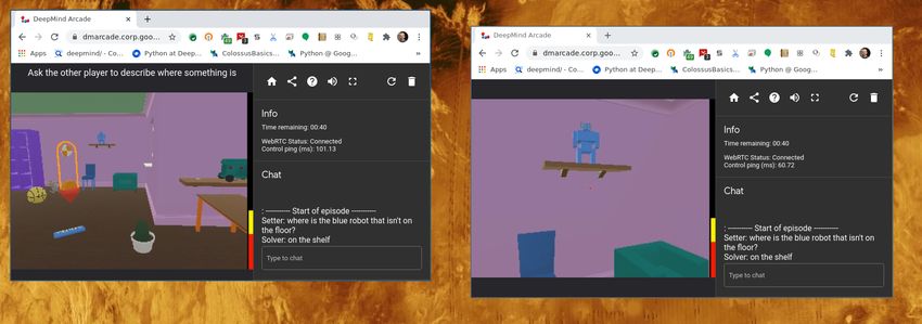
1     Introduction
Humans are an interactive species. We interact with the physical world and with one an-
other. We often attribute our evolved social and linguistic complexity to our intelligence,
but this inverts the story: the shaping forces of large-group interactions selected for these
capacities (Dunbar, 1993), and these capacities are much of the material of our intelligence.
To build artificial intelligence capable of human-like thinking, we therefore must not only
grapple with how humans think in the abstract, but also with how humans behave as physi-
cal agents in the world and as communicative agents in groups. Our study of how to create
artificial agents that interact with humans therefore unifies artificial intelligence with the
study of natural human intelligence and behaviour.
    This work initiates a research program whose goal is to build embodied artificial agents
that can perceive and manipulate the world, understand and produce language, and react
capably when given general requests and instructions by humans. Such a holistic research
program is consonant with recent calls for more integrated study of the “situated” use of
language (McClelland et al., 2019; Lake and Murphy, 2020). Progress towards this goal
could greatly expand the scope and naturalness of human-computer interaction (Winograd,
1972; Card et al., 1983; Branwen, 2018) to the point that interacting with a computer or a
robot would be much like interacting with another human being – through shared attention,
gesture, demonstration, and dialogue (Tomasello, 2010; Winograd, 1972).
    Our research program shares much the same spirit as recent work aimed to teach vir-
tual or physical robots to follow instructions provided in natural language (Hermann et al.,
2017; Lynch and Sermanet, 2020) but attempts to go beyond it by emphasising the inter-
active and language production capabilities of the agents we develop. Our agents interact
with humans and with each other by design. They follow instructions but also generate
them; they answer questions but also pose them.

2     Our Research Program
2.1    The Virtual Environment
We have chosen to study artificial agent interactions in a 3D virtual environment based on
the Unity game engine (Ward et al., 2020). Although we may ultimately hope to study in-
teractive physical robots that inhabit our world, virtual domains enable integrated research
on perception, control, and language, while avoiding the technical difficulties of robotic
hardware, making them an ideal testing ground for any algorithms, architectures, and eval-
uations we propose.
    The environment, which we call “the Playroom,” comprises a randomised set of rooms
with children’s toys and domestic objects (Figure 1). The robotic embodiment by which
the agent interacts with the world is a “mobile manipulator” – that is, a robot that can
move around and reposition objects. This environment supports a broad range of possible
tasks, concepts, and interactions that are natural and intuitive to human users. It has con-

                                              2
A B
C
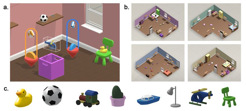
Figure 1: The “Playroom”. The 3-D “Playroom” environment comprises a randomised set of
rooms with children’s toys and domestic objects, as well as containers, shelves, furniture, windows,
and doors. The diversity of the environment enables interactions involving reasoning about space
and object relations, ambiguity of references, containment, construction, support, occlusion, and
partial observability. Agents interact with the world by moving around, manipulating objects, and
speaking to each other. A. Depicts a simple interaction wherein the orange solver agent is placing
a helicopter into a container while the blue setter agent watches on. B. Shows four random instan-
tiations of the Playroom, each with a unique combination and arrangement of objects and furniture.
C. A sampling of the types of objects available in the room.
tainers, shelves, furniture, windows, and doors whose initial positions vary randomly each
episode. There are diverse toys and objects that can be moved and positioned. The rooms
are L-shaped, creating blocked lines of sight, and have randomly variable dimensions. As
a whole, the environment supports interactions that involve reasoning about space and ob-
ject relations, ambiguity of references, containment, construction, support, occlusion, and
partial observability. The language referring to this world can involve instructed goals,
questions, or descriptions at different levels of specificity. Although the environment is
simple compared to the real world, it affords rich and combinatorial interactions.
2.2 Learning to Interact
We aim to build agents that can naturally interact with and usefully assist humans. As a first
step, one might consider optimising for this outcome directly. A critical prerequisite is a
metric measuring “useful” interactions. Yet defining such a metric is a thorny issue because
what comprises “useful” (or, simply, “good”) is generally ambiguous and subjective. We
need a way to measure and make progress without interminable Socratic debate about the
meaning of “good” (Adam et al., 1902).
Suppose we do not have such an explicit rule-based metric to apply to any interaction.
3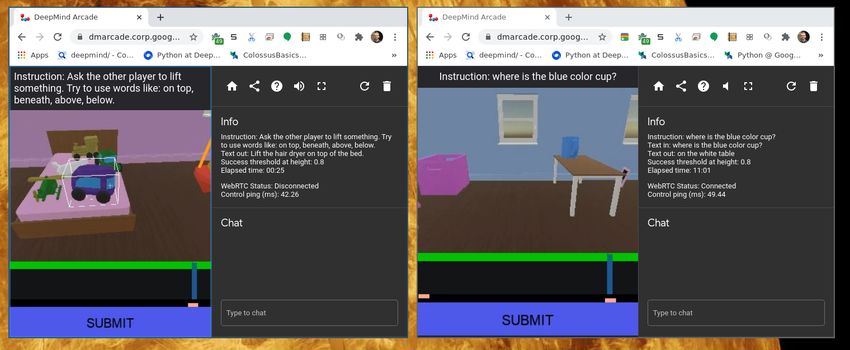
In principle, we can overcome the issue of the subjectivity of evaluation by embracing it:
we can instead rely on a human evaluator’s or collective of evaluators’ judgements of the
utility of interactions. This resolves the problem of codifying these value judgements a
priori. However, additional challenges remain. For the sake of argument, let’s first suppose
that an evaluator is only tasked with judging very unambiguous cases of success or failure.
In such a scenario, the efficiency of improving an agent by issuing evaluative feedback
depends critically on the intelligence of the agent being evaluated. Consider the two cases
below:
    If the agent is already intelligent (for example, it is another human), then we can expect
the ratio of successes to failures to be moderately high. If the evaluator can unambiguously
evaluate the behaviour, then their feedback can be informative. The mutual information
between behaviour and evaluation is upper-bounded by the entropy in the evaluation1 , and
this mutual information can be used to provide feedback to the agent that discriminates
between successes and failures.
    If, however, the agent is not already intelligent (for example, it is an untrained agent),
then we can expect the ratio of successes to failures to be extremely low. In this case,
almost all feedback is the same and, consequently, uninformative; there is no measurable
correlation between variations in agent behaviour and variations in the evaluation. As tasks
increase in complexity and duration, this problem only becomes more severe. Agents must
accidentally produce positive behaviour to begin to receive discriminative feedback. The
number of required trials is inversely related to the probability that the agent produces a
reasonable response on a given trial. For a success probability of 10−3 , the agent needs
approximately 1,000 trials before a human evaluator sees a successful trial and can provide
feedback registering a change in the optimisation objective. The data required then grow
linearly in the time between successful interactions.
    Even if the agent fails almost always, it may be possible to compare different trials
and to provide feedback about “better” and “worse” behaviours produced by an agent
(Christiano et al., 2017). While such a strategy can provide a gradient of improvement
from untrained behaviour, it is still likely to suffer from the plateau phenomenon of in-
discernible improvement in the early exploration stages of reinforcement learning (Kakade
et al., 2003). This will also dramatically increase the number of interactions for which eval-
uators need to provide feedback before the agent reaches a tolerable level of performance.
    Regardless of the actual preferences (or evaluation metric) of a human evaluator, fun-
damental properties of the reinforcement learning problem suggest that performance will
remain substandard until the agent begins to learn how to behave well in exactly the same
distribution of environment states that an intelligent expert (e.g., another human) is likely
to visit. This fact is known as the performance difference lemma (Kakade et al., 2003).
Formally, if π ∗ (s) is the state distribution visited by the expert, π ∗ (a | s) is the action dis-
tribution of the expert, V π is the average value achieved by the agent π, and Qπ (s, a) is the
value achieved in a state if action a is chosen, then the performance gap between the expert
   1
    For any two random variables B (e.g. a behavioural episode of actions taken by humans) and Y (e.g. a
binary evaluation), I[B; Y ] = H[Y ] − H[Y | B] ≤ H[Y ].

                                                   4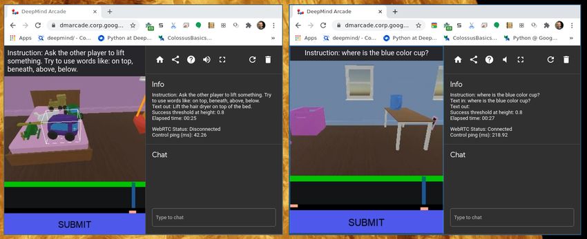
π ∗ and the agent π is
                     ∗
                                X               X
                 Vπ −Vπ =             π ∗ (s)    (π ∗ (a | s) − π(a | s))Qπ (s, a).
                                  s              a

That is, as long as the expert is more likely to choose a good action (with larger Qπ (s, a))
in the states it likes to visit, there will be a large performance difference. Unfortunately,
the non-expert agent has quite a long way to go before it can select those good actions,
too. Because an agent training from scratch will visit a state distribution π(s) that is sub-
stantially different from the expert’s π ∗ (s) (since the state distribution is itself a function of
the policy), it is therefore unlikely to have learned how to pick good actions in the expert’s
favoured states, neither having visited them nor received feedback in them. The problem is
vexed: to learn to perform well, the agent must often visit common expert states, but doing
so is tantamount to performing well. Intuitively, this is the cause of the plateau phenomenon
in RL. It poses a substantial challenge to “human-in-the-loop” methods of training agents
by reward feedback, where the human time required to evaluate and provide feedback can
be tedious, expensive, and can bottleneck the speed with which the AI can learn. The
silver lining is that, while this theorem makes a serious problem apparent, it also points
toward a resolution: if we can find a way to generally make π(a | s) = π ∗ (a | s), then the
performance gap disappears.
     In sum, while we could theoretically appeal to human judgement in lieu of an explicit
metric to train agents to interact, it would be prohibitively inefficient and result in a substan-
tial expenditure of human effort for little gain. For training by human evaluation to merit
further consideration, we should first create agents whose responses to a human evalua-
tor’s instructions are satisfactory a larger fraction of the time. Ideally, the agent’s responses
are already very close to the responses of an intelligent, cooperative person who is try-
ing to interact successfully. At this point, human evaluation has an an important role to
play in adapting and improving the agent behaviour by goal-directed optimisation. Thus,
before we collect and learn from human evaluations, we argue for building an intelligent
behavioural prior: namely, a model that produces human-like responses in a variety of
interactive contexts.
     Building a behavioural prior and demonstrating that humans judge it positively dur-
ing interaction is the principal achievement of this work. We turn to imitation learning
to achieve this, which directly leverages the information content of intelligent human be-
haviour to train a policy.

2.3    Collecting Data for Imitation Learning
Imitation learning has been successfully deployed to build agents for self-driving cars
(Pomerleau, 1989), robotics and biomimetic motor control (Schaal, 1999), game play (Sil-
ver et al., 2016; Vinyals et al., 2019), and language modeling (Shannon, 1951). Imitation
learning works best when humans are able to provide very good demonstrations of be-
haviour, and in large supply. For some domains, such as pure text natural language pro-
cessing, large corpora exist that can be passively harvested from the internet (Brown et al.,

                                                     5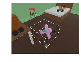
2020). For other domains, more targeted data collection is currently required. Training
agents by imitation learning in our domain requires us to devise a protocol for collecting
human interaction data, and then to gather it at scale. The dataset we have assembled con-
tains approximately two years of human-human interactions in real-time video and text.
Measured crudely in hours (rather than in the number of words or the nature of utterances),
it matches the duration of childhood required to attain oral fluency in language.
    To build an intelligent behavioural prior for an agent acting in the Playroom, we could
theoretically deploy imitation learning on free-form human interactions. Indeed, a small
fraction of our data was collected this way. However, to produce a data distribution repre-
senting certain words, skills, concepts, and interaction types in desirable proportions, we
developed a more controlled data collection methodology based on events called language
games.2
    We categorised the space of interactions into four basic types: question and answer
(Q&A), instruction-following, play, and dialogue (Figure 2). For this work, we have fo-
cused exclusively on the first two. Within each type, we framed several varieties of prede-
fined prompts. Prompts included, “Ask the other player to bring you one or more objects,”
and, “Ask the other player whether a particular thing exists in the room.” We used 24
base prompts and up to 10 “modifiers” (e.g., “Try to refer to objects by color”) that were
appended to the base prompts to provide variation and encourage more specificity. One
example of a prompt with a modifier was: “Ask the other player to bring you one or more
object. Try to refer to objects by color.”
    Human participants were divided into two groups: setters and solvers. Setters received
a prompt and were responsible for issuing an instruction based on it. Solvers were respon-
sible for following instructions. Each episode in which a human setter was prompted to
provide an instruction to a human solver is what we call a language game (Figure 19). In
each language game, a unique room was sampled from a generative model that produces
random rooms, and a prompt was sampled from a list and shown to the setter. The human
setter was then free to move around the room to investigate the space. When ready, the
setter would then improvise an instruction based on the prompt they received and would
communicate this instruction to the solver through a typed chat interface (Figure 18). The
setter and solver were given up to two minutes for each language game.
    The role of the setter was therefore primarily to explore and understand the situational
context of the room (its layout and objects) and to initiate diverse language games con-
strained by the basic scaffolding given by the prompt (Figure 2). By defining a simple set
of basic prompts, we could utilise humans’ creative ability to conjure interesting, valid in-
structions on-the-fly, with all the nuance and ambiguity that would be impossible to define
programmatically. While the language game prompts constrained what the setters ought to
instruct, setters and solvers were both free to use whatever language and vocabulary they
liked. This further amplified the linguistic diversity of the dataset by introducing natural
variations in phrasing and word choice. Consider one example, shown in the lower panel of
Figure 3: the setter looks at a red toy aeroplane, and, prompted to instruct the solver to lift
   2
       Inspired by Wittgenstein’s ideas about the utility of communication (Wittgenstein, 1953).

                                                       6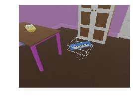
Interaction      Prompt                           Instruction

                                        Count the lamps on the floor
                              Count
                                        How many toys are on the bed?

               Q&A                      Can you please count the number of blue things
                              Color

                                        Where is the blue duck?
            Instruction     Location

                                        Please place any toy train beside a toy car
                Play        Position

                                        Lift any object which is close to the magenta table
             Dialogue          Lift
                                        Can you lift the rocket on the bookshelf?
                 ...

                                ...

             Not explored               Grab the red toy on the table and lift it
             in this work
                                Go      Go as far away from the table as possible

             Provided by environment         Generated by setter agent online during episode

Figure 2: Generating Diverse Interactions. Interactions in the Playroom could take myriad
forms. To encourage diverse interactions in the Playroom, we provided prompts (in orange) to
humans which they expanded into specific language instructions (in red) for the other human or
agent. Prompts shown here are short forms: e.g. Lift corresponded to “Ask the other player to lift
something in the room,” Color corresponded to “Ask the other player about the color of something
in the room.”

something, asks the solver to “please lift the object next to the magenta table,” presumably
referring to the aeroplane. The solver then moves to the magenta table and instead finds a
blue keyboard, which it then lifts. This constituted a successful interaction even though the
referential intention of the instruction was ambiguous.
    Altogether, we collected 610,608 episodes of humans interacting as a setter-solver pair.
From this total we allocated 549,468 episodes for training, and 61,140 for validation.
Episodes lasted up to a maximum of 2 minutes (3,600 steps), with a mean and standard
deviation of 55 ± 25s (1,658 ± 746 steps). The relative proportion of language games can
be found in Table 6 in the Appendix. Setters took 26 ± 16s (784 ± 504 steps) to pose a
task for a solver, given the environment prompt (which was communicated at the start of an
episode). In the 610,608 episodes there were 320,144 unique setter utterances, and 26,023
unique solver utterances, with an average length of 7.5 ± 2.5 words and a maximum length
of 29 words for setters. To put it another way, this signifies that there are 320,144 unique
tasks instructed in the dataset. For solvers, the average length was 4.1 ± 2.4 and a maxi-
mum length of 26. Upon receiving a setter instruction, the time solvers took to complete
the task was 28 ± 18s (859 ± 549 steps). Figure 4 depicts the average action composi-
tion for a solver in an episode. Notably, the density of actions was low, and when actions
were taken, the distribution of action choice was highly skewed. This was even more
pronounced for language emissions (Figure 11A), where approximately one utterance was

                                                 7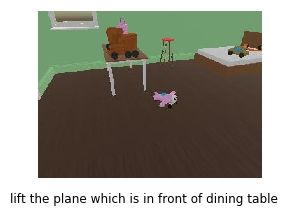
Prompt: Ask the other player to lift something
                                                                   2
          Solver                                                        1. Setter Gives Instruction        2. Solver Completes Task
   Move
   Look
   Grab
  Speak
                                                  1
          Setter
   Move
   Look
   Grab
  Speak
                                                                       "lift the plane which is in front
          0                 500            1000                1500            of the dining table"
                              Episode Timestep

                                                               2
          Solver
   Move                                                                 1. Setter Gives Instruction        2. Solver Completes Task
   Look
   Grab
  Speak
                        1
          Setter
   Move
   Look
   Grab
  Speak
                                                                       "please lift the object next to
          0                 1000           2000                3000         the magenta table"
                              Episode Timestep

Figure 3: Example Trajectories. In these two human-human episodes, the setter was prompted
to ask the solver to lift an object in the room. In the top example, the setter sets the task and the
solver completes it in a straightforward manner. In the bottom example, there is some ambiguity:
the setter was presumably referring to the red airplane on the ground, but the solver proceeded to
lift the blue keyboard, which was also near the magenta table. The task was nevertheless completed
successfully.

made per episode for setters, with word choices following a long-tailed distribution for a
vocabulary of approximately 550 words.

2.4       Agent Architecture
2.4.1         Action Representation
Our agents control the virtual robot in much the same way as the human players. The
action space is multidimensional and contains a continuous 2D mouse look action. The
agent space also includes several keyboard buttons, including forward, left, backward, right
(corresponding to keys ‘WASD’), along with mixtures of these keys (Figure 3). Finally, a
grab action allows the agent to grab or drop an object. The full details of the observation
and action spaces are given in Appendix 3.4.
    The agent operates in discrete time and produces 15 actions per second. These actions
are produced by a stochastic policy, a probability distribution, π, defined jointly over all

                                                               8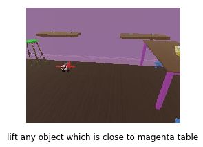
Action Sparsity                                     Move Actions                                  Look Actions
                                                                                                          1
        Move                                           Forward
                                                          Back

                                                                                               Vertical
                                          No-Op            Left
        Look                                                                                              0
                                          Op              Right

        Grab                                       Forward Left
                                                  Forward Right
                                                                                                          -1
            0.0        0.5          1.0                      0.00 0.10 0.05 0.15                               -1        0         1
                   Frequency                                           Frequency                                     Horizontal

Figure 4: Action Composition. Across each of the move, look, and grab actions we observed
a skewed distribution with respect to the chosen actions (middle, right), and whether an action or
no-op is chosen (left). For the move action, “forward” is heavily represented, whilst look actions
are clustered mainly around the origin (corresponding to small shifts in gaze direction), and along
the borders (corresponding to large rotations). Each action is relatively rare in the entire trajectory,
as seen by the proportion of no-ops to ops.

the action variables produced in one time step, a: π(a) = π(look, key, grab) (At times, we
may use the words agent and policy interchangeably, but when we mean to indicate the
conditional distribution of actions given observations, we will refer to this as the policy
exclusively.) In detail, we include no-operation (“no-op”) actions to simplify the pro-
duction of a null mouse movement or key press. Although we have in part based our
introductory discussion on the formalism of fully-observed Markov Decision Processes,
we actually specify our interaction problem more generally. At any time t in an episode,
the policy distribution is conditioned on the preceding perceptual observations, which we
denote o≤t ≡ (o0 , o1 , . . . , ot ). The policy is additionally autoregressive. That is, the agent
samples one action component first, then conditions the distribution over the second action
component on the choice of the first, and so on. If we denote the choice of the look no-op
                     (0)                                        (1)
action at time t as at , the choice of the look action as at , the choice of the key no-op as
  (2)                                (3)
at , the choice of the key as at , and so on, the action distribution is jointly expressed as:
                                                          K
                                                          Y              (k)            (
2.4.2 Perception and Language
Agents perceive the environment visually using “RGB” pixel input at resolution of 96 × 72.
When an object can be grasped by the manipulator, a bounding box outlines the object
(Figures 1, 3, & 4). Agents also process text inputs coming from either another player
(including humans), from the environment (agents that imitate the setter role must process
the language game prompt), or from their own language output at the previous time step.
Language input is buffered so that all past tokens up to a buffer length are observed at
once. We will denote the different modalities of vision, language input arriving from the
language game prompt, language input coming from the other agent, and language input
coming from the agent itself at the last time step as oV , oLP , and oLO , and oLS , respectively.
Language output is sampled one token at a time, with this step performed after the
autoregressive movement actions have been chosen. The language output token is observed
by the agent at the next time step. We process and produce language at the level of whole
words, using a vocabulary consisting of the approximately 550 most common words in the
human data distribution (Section 10) and used an ‘UNK’ token for the rest.
2.4.3 Network Components
The agent architecture (Figure 5) uses a ResNet (He et al., 2016) for vision. At the highest
level of the ResNet, a spatial map of dimensions (width × height × number-of-channels) is
produced. The vectors from all the width×height positions in this spatial array are concate-
nated with the embeddings of the language input tokens, which include words comprising
the inter-agent communication, the prompt delivered from the environment (to the setter
only), and previous language emissions. These concatenated vectors are jointly processed
by a transformer network (Vaswani et al., 2017), which we refer to as the multi-modal
transformer (MMT). The output of the MMT consists of a mean-pooling across all output
embeddings, concatenated with dedicated output embeddings that function much like the
“CLS” embedding in the BERT model (Devlin et al., 2018) (see Section 3.2 in the Appendix
for more information). This output provides the input to an LSTM memory, which in turn
provides the input to smaller networks that parameterise the aforementioned policies.
2.5 Learning
Our approach to training interactive agents combines diverse techniques from imitation
learning with additional supervised and unsupervised learning objectives to regularise rep-
resentations. We first explain the basic principles behind each method, then explain how
they are brought together.
2.5.1 Behavioural Cloning
The most direct approach to imitation learning, known as behavioural cloning (BC) (Pomer-
leau, 1989; Osa et al., 2018), frames the problem of copying behaviour as a supervised
10Multi-Modal Transformer
LSTM
xN
ResNet Flatten
Image Movement Policy
...
...
96x72 RGB (Move Look Grab, No-Op)
Autoregressive
Prompt Tokenize & Embed Language Policy
...
...
Prev. Lang. (Word, No-Op)
Inter-Agent Comms.
Text String
Figure 5: Agent Architecture. The agent receives both RGB images and text strings as inputs.
The former gets encoded through a ResNet, and the latter are tokenized by word using a custom
vocabulary, and subsequently embedded as distributed vectors. Together the ResNet “hyper-pixels”
and tokenized words comprise a set of vectors that is the input to a multi-modal transformer. The
transformer’s output provides the input to an LSTM, which in turn provides input to the motor and
language policies.
sequence prediction problem (Graves, 2013). Recalling the discussion of the performance
difference lemma, behavioural cloning is an approach that tries to make π(a | s) = π ∗ (a |
s), or, in our case, π(at | o≤t ) = π ∗ (at | o≤t ). It requires a dataset of observation and
action sequences produced by expert demonstrators.
A temporal observation sequence o≤T ≡ (o0 , o1 , o2 , . . . , oT ) and a temporal action
sequence a≤T ≡ (a0 , a1 , a2 , . . . , aT ) together comprise a trajectory. (Length, or trajectory
length, refers to the number of elements in the observation or action sequence, and while
trajectory lengths can vary, for simplicity we develop the fixed length case.) The dataset is
distributed according to some unknown distribution π ∗ (o≤T , a≤T ). For language games, we
constructed separate datasets of setter trajectories and solver trajectories. The loss function
for behavioural cloning is the (forward) Kullback-Leibler divergence between π ∗ and πθ :
LBC (θ) = KL [π ∗ kπθ ]
π ∗ (o≤T , a≤T )
= Eπ∗ (o≤T ,a≤T ) ln
πθ (o≤T , a≤T )
= const(θ) − Eπ∗ (o≤T ,a≤T ) [ln πθ (o≤T , a≤T )] ,
where const(θ) collects the demonstrator distribution entropy term, which is a constant in-
dependent of the policy parameters. The policy trajectory distribution πθ (o≤T , a≤T ) is a
product of conditional distributions from each time step. The product alternates between
terms that are a function of the policy directly, πθ (at | o≤t , abroken down by time step:
" T
#
Y
LBC (θ) = −Eπ∗ (o≤T ,a≤T ) ln pENV (ot | othe training data, πθ (at | oUNSEEN,≤t ), the desired response is nominally undefined and must
be inferred by appropriate generalisation.
In the Playroom (or indeed, in any human-compatible environment), we know that
pixels are grouped into higher-order structures that we perceive as toys, furniture, the back-
ground, etc. These higher-order structures are multi-scale and include the even higher-
order spatial relationships among the objects and features in the room. Together, these
perceptual structures influence human behaviour in the room. Our regularisation proce-
dures aim to reduce the number of degrees of freedom in the input data source and the
network representations, while preserving information that is correlated with attested hu-
man behaviour. These regularisation procedures produce representations that effectively
reduce the discriminability of some pairs of observation sequences (oi,≤t , oj,≤t ) while in-
creasing the discriminability of others. The geometry of these representations then shapes
how the policy network infers its responses, and how it generalises to unseen observations.
We use two kinds of regularisation, both of which help to produce visual representations
that improve BC agents with respect to our evaluation metrics. The first regularisation,
which we call Language Matching (LM), is closely related to the Contrastive Predictive
Coding algorithm (van den Oord et al., 2018; Hénaff et al., 2019) and Noise Contrastive
Estimation (Gutmann and Hyvärinen, 2010) and helps produce visual representations re-
flecting linguistic concepts. A classifier Dθ is attached to the agent network and provided
input primarily from the mean-pooling vector of the MMT. It is trained to determine if the
visual input and the solver language input (i.e., the instruction provided by the setter) come
from the same episode or different episodes (see Appendix section 3.2):
B T
LM 1 XX V LO V LO
L (θ) = − ln Dθ (on,t , on,t ) + ln 1 − Dθ (on,t , oS HIFT(n),t ) , (2)
B n=1 t=0
where B is the batch size and S HIFT(n) is the n-th index after a modular shift of the in-
tegers: 1 → 2, 2 → 3 . . . , B → 1. The loss is “contrastive” because the classifier must
distinguish between real episodes and decoys. To improve the classifier loss, the visual en-
coder must produce representations with high mutual information to the encoded language
input. We apply this loss to data from human solver demonstration trajectories where there
is often strong alignment between the instructed language and the visual representation:
for example, “Lift a red robot” predicts that there is likely to be a red object at the centre
of fixation, and “Put three balls in a row” predicts that three spheres will intersect a ray
through the image.
The second regularisation, which we call the “Object-in-View” loss (OV), is designed
very straightforwardly to produce visual representations encoding the objects and their
colours in the frame. We build a second classifier to contrast between strings describ-
ing coloured objects in frame versus fictitious objects that are not in frame. To do this,
we use information about visible objects derived directly from the environment simulator,
although equivalent results could likely be obtainable by conventional human segmentation
and labeling of images (Girshick, 2015; He et al., 2017). Notably, this information is only
present during training, and not at inference time.
13Together, we refer to these regularising objective functions as “auxiliary losses.”
2.5.3 Inverse Reinforcement Learning
In the Markov Decision Process formalism, we can write the behavioural cloning objective
another way to examine the sense in which it tries to make the agent imitate the demonstra-
tor:
LBC (θ) = Eπ∗ (s) [KL [π ∗ (a | s)kπθ (a | s)]] .
The imitator learns to match the demonstrator’s policy distribution over actions in the ob-
servation sequences generated by the demonstrator. Theoretical analysis of behavioural
cloning (Ross et al., 2011) suggests that errors of the imitator agent in predicting the demon-
strator’s actions lead to a performance gap that compounds.3 The root problem is that each
mistake of the imitator changes the distribution of future states so that πθ (s) differs from
π ∗ (s). The states the imitator reaches may not be the ones in which it has been trained to
respond. Thus, a BC-trained policy can “run off the rails,” reaching states it is not able to
recover from. Imitation learning algorithms that also learn along the imitator’s trajectory
distribution can reduce this suboptimality (Ross et al., 2011).
The regularisation schemes presented in the last section can improve the generalisation
properties of BC policies to novel inputs, but they cannot train the policy to exert active con-
trol in the environment to attain states that are probable in the demonstrator’s distribution.
By contrast, inverse reinforcement learning (IRL) algorithms (Ziebart, 2010; Finn et al.,
2016) attempt to infer the reward function underlying the intentions of the demonstrator
(e.g., which states it prefers), and optimise the policy itself using reinforcement learning to
pursue this reward function. IRL can avoid this failure mode of BC and train a policy to
“get back on the rails” (i.e., return to states likely in the demonstrator’s state distribution;
see previous discussion on the performance difference lemma). For an instructive example,
consider using inverse reinforcement learning to imitate a very talented Go player. If the
reward function that is being inferred is constrained to observe only the win state at the end
of the game, then the estimated function will encode that winning is what the demonstra-
tor does. Optimising the imitator policy with this reward function can then recover more
information about playing Go well than was contained in the dataset of games played by
the demonstrator alone. Whereas a behavioural cloning policy might find itself in a losing
situation with no counterpart in its training set, an inverse reinforcement learning algorithm
can use trial and error to acquire knowledge about how to achieve win states from unseen
conditions.
Generative Adversarial Imitation Learning (GAIL) (Ho and Ermon, 2016) is an algo-
rithm closely related to IRL (Ziebart, 2010; Finn et al., 2016). Its objective trains the
3
Under relatively weak assumptions (bounded task rewards per time step), the suboptimality for BC is
linear in the action prediction error rate but up to quadratic in the length of the episode T , giving O(T 2 ).
The performance difference would be linear in the episode length, O(T ), if each mistake of the imitator
incurred a loss only at that time step; quadratic suboptimality means roughly that an error exacts a toll for
each subsequent step in the episode.
14policy to make the distribution πθ (s, a) match π ∗ (s, a). To do so, GAIL constructs a surro-
gate model, the discriminator, which serves as a reward function. The discriminator, Dφ ,
is trained using conventional cross entropy to judge if a state and action pair is sampled
from a demonstrator or imitator trajectory:
LDISC (φ) = −Eπ∗ (s,a) [ln Dφ (s, a)] − Eπθ (s,a) [ln(1 − Dφ (s, a))] .
π (s,a) ∗
The optimal discriminator, according to this objective, satisfies Dφ (s, a) = π∗ (s,a)+π θ (s,a)
.4
We have been deliberately careless about defining π(s, a) precisely but rectify this now.
In the discounted case, it can be defined as the discounted P summed probability of being
t
in a state and producing an action: π(s, a) ≡ (1 − γ) t γ p(st = s | π)π(a | s). The
objective of the policy is to minimise the classification accuracy of the discriminator, which,
intuitively, should make the two distributions as indiscriminable as possible: i.e., the same.
Therefore, the policy should maximise
J GAIL (θ) = −Eπθ (s,a) [ln(1 − Dφ (s, a))] .
This is exactly a reinforcement learning objective with per time step reward function r(s, a) =
− ln(1 − Dφ (s, a)). It trains the policy during interaction with the environment: the ex-
pectation is under the imitator policy’s distribution, not the demonstrator’s. Plugging in the
optimal discriminator on the right-hand side, we have
GAIL πθ (s, a)
J (θ) ≈ −Eπθ (s,a) ln ∗ .
π (s, a) + πθ (s, a)
At the saddle point, optimised both with respect to the discriminator and with respect to
the policy, one can show that πθ (s, a) = π ∗ (s, a).5 GAIL differs from traditional IRL
algorithms, however, because the reward function it estimates is non-stationary: it changes
as the imitator policy changes since it represents information about the probability of a
trajectory in the demonstrator data compared to the current policy.
GAIL provides flexibility. Instead of matching πθ (s, a) = π ∗ (s, a), one can instead
attempt to enforce only that πθ (s) = π ∗ (s) (Merel et al., 2017; Ghasemipour et al., 2020).
We have taken this approach both to simplify the model inputs, and because it is sufficient
for our needs: behavioural cloning can be used to imitate the policy conditional distribution
π ∗ (a | s), while GAIL can be used to imitate the distribution over states themselves π ∗ (s).
In this case the correct objective functions are:
LDISC (φ) = −Eπ∗ (s) [ln Dφ (s)] − Eπθ (s) [ln(1 − Dφ (s))] ,
J GAIL (θ) = −Eπθ (s,a) [ln(1 − Dφ (s))] .
4
As was noted in Goodfellow et al. (2014) and as is possible to derive by directly computing the stationary
point with respect to Dφ (s, a): π ∗ (s, a)/Dφ (s, a) − πθ (s, a)/(1 − Dφ (s,P a)) = 0, etc.
5
Solving the constrained optimisation problem J GAIL (θ) + λ[ a πθ (s, a) − 1] shows that
πθ (s,a) ∗
π ∗ (s,a)+πθ (s,a) = const for all s, a. Therefore, πθ (s, a) = π (s, a).
15Multi-Modal Transformer Temporal
xN Transformer
ResNet Flatten t-N MLP
Image Augment
...
...
reduce
Crop, Rotate t-2 Discriminator
...
...
96x72 RGB Shear, Translate t-1
reduce Loss
Prompt xN
Tokenize & Embed
...
...
Prev. Lang.
Language Matching
Inter-Agent Comms. Loss
Text String
Figure 6: GAIL Discriminator Architecture: The discriminator receives the same inputs as the
agent, RGB images and text strings, and encodes them with similar encoders (ResNet, text em-
bedder, and Multi-Modal Transformer) into a single summary vector. The encoded inputs are then
processed by a Temporal Transformer that has access to the summary vectors from previous time
steps. The mean-pooled output of this transformer is then passed through an MLP to obtain a single
output representing the probability that the observation sequence is part of a demonstrator trajectory.
The encoders are simultaneously trained by the auxiliary Language Matching objective.
In practice, returning to our Playroom setting with partial observability and two agents
interacting, we cannot assume knowledge of a state st . Instead, we supply the discriminator
with observation sequences st ≈ (ot−sk , ot−s(k−1) , . . . , ot ) of fixed length k and stride s;
the policy is still conditioned as in Equation 1.
These observation sequences are short movies with language and vision and are con-
sequently high-dimensional. We are not aware of extant work that has applied GAIL to
observations this high-dimensional (see Li et al. (2017); Zolna et al. (2019) for applica-
tions of GAIL to simpler but still visual input), and, perhaps, for good reason. The dis-
criminator classifier must represent the relative probability of a demonstrator trajectory
compared to an imitator trajectory, but with high-dimensional input there are many unde-
sirable classification boundaries the discriminator can draw. It can use capacity to over-fit
spurious coincidences: e.g., it can memorise that in one demonstrator interaction a pixel
patch was hexadecimal colour #ffb3b3, etc., while ignoring the interaction’s semantic con-
tent. Consequently, regularisation, as we motivated in the behavioural cloning context,
is equally important for making the GAIL discriminator limit its classification to human-
interpretable events, thereby giving reward to the policy if it acts in ways that humans also
think are descriptive and relevant. For the GAIL discriminator, we use a popular data aug-
mentation technique RandAugment (Cubuk et al., 2020) designed to make computer vision
more invariant. This technique stochastically perturbs each image that is sent to the vi-
sual ResNet. We use random cropping, rotation, translation, and shearing of the images.
These perturbations substantially alter the pixel-level visual input without altering human
understanding of the content of the images or the desired outputs for the network to pro-
duce. At the same time, we use the same language matching objective we introduced in
the behavioural cloning section, which extracts representations that align between vision
16and language. This objective is active only when the input to the model is demonstrator
observation sequence data, not when the imitator is producing data.
The architecture of the discriminator is shown in Figure 6. RandAugment is applied
to the images, and a ResNet processes frames, converting them into a spatial array of vec-
tor embeddings. The language is also similarly embedded, and both are passed through a
multi-modal transformer. No parameters are shared between the reward model and policy.
The top of the MMT applies a mean-pooling operation to arrive at a single embedding per
time step, and the language matching loss is computed based on this averaged vector. Sub-
sequently, a second transformer processes the vectors that were produced across time steps
before mean-pooling again and applying a multi-layer perceptron classifier representing
the discriminator output.
Auxiliary learning
Behavioural cloning
Policy
Forward Inverse
Human RL RL
demonstrations
Reward
model
Auxiliary learning
Figure 7: Training schematic. We train policies using human demonstrations via a mixture of
behavioural cloning and reinforcement learning on a learned discriminator reward model. The re-
ward model is trained to discriminate between human demonstrations (positive examples) and agent
trajectories (negative examples). Both the policy and the reward model are regularised by auxiliary
objectives.
Figure 7 summarises how we train agents. We gather human demonstrations of inter-
active language games. These trajectories are used to fit policies by behavioural cloning.
We additionally use a variant of the GAIL algorithm to train a discriminator reward model,
classifying trajectories as generated by either the humans or a policy. Simultaneously, the
policy derives reward if the discriminator classifies its trajectory as likely to be human.
Both the policy and discriminator reward model are regularised by auxiliary learning ob-
jectives.
In Figure 8, we compare the performance of our imitation learning algorithms applied
to a simplified task in the Playroom. A dataset was collected of a group of subjects in-
structed using synthetic language to put an object in the room on the bed. A programmatic
171.0
Performance
BG·A
B·A
0.5 BG
B
G·A
0.0
0 1 2 3 4 5
1e8
Training Steps
Figure 8: Comparison of Imitation Learning Methods on Simple ‘Put X on Bed’ Task. In this
task, an agent is instructed to put an object in the room on the bed using synthetic language. The
data comprised 40, 498 human episodes pre-selected based on success. The GAIL agent (G·A),
even with auxiliary loss regularisation of the agent and discriminator, failed to learn, while the
simple BC (B) agent learned to retrieve objects at random but did not identify the correct one.
Combining BC with GAIL (BG) or BC with auxiliary regularisation (B·A) improved performance.
Further performance was reached by combining GAIL, BC, and auxiliary losses (BG·A). Note that
certain possible comparison models were not run here, including simple GAIL (G), and variations
that would use auxiliary losses on the agent but not the discriminator and vice versa.
reward function that detects what object is placed on the bed was used to evaluate perfor-
mance. Under no condition was the reward function used to train any agent. The agent and
discriminator trained by GAIL with the regularisation (G·A; ‘A’ denotes the inclusion of
‘auxiliary’ regularisation, including the LM loss and RandAugment on the discriminator)
was unable to improve beyond its random initialisation. The behavioural cloning agent (B)
was slightly better but did not effectively understand the task: its performance implies it
picked up objects at random and put them on the bed. Combining the behavioural cloning
with GAIL (BG) by simply adding the loss terms together achieved reasonable results,
implying that GAIL was better at reshaping a behavioural prior than structuring it from
scratch. However, behavioural cloning with the additional regularisation (B·A; LM and
OV on the policy) achieved essentially the same or better results. Adding the auxiliary
LM and OV losses to behavioural cloning and the GAIL discriminator was the best of all
(BG·A). While this task is simple, we will show that this rough stratification of agents per-
sisted even when we trained agents with complicated language games data and reported
scores based on human evaluations.
2.5.4 Interactive Training
While this training recipe is sufficient for simple tasks defined with programmed language
and reward, to build agents from language games data requires further innovation to model
both the setter and solver behaviour and their interaction. In this work, we train one single
agent that acts as both a setter and a solver, with the agent engaged as a setter if and only
18Input modalities Training algorithms
Name Vision Language BC GAIL Setter replay Auxiliary losses
BGR·A 3 3 3 3 3 3
BG·A 3 3 3 3 7 3
BG 3 3 3 3 7 7
G·A 3 3 7 3 7 7
B·A 3 3 3 7 7 3
B 3 3 3 7 7 7
B(no vis.) 7 3 3 7 7 7
B(no lang.) 3 7 3 7 7 7
Table 1: Agent Nomenclature. Note that “no vis.” and “no lang.” indicate no vision and language
input, respectively.
if the language prompt oLP is non-empty. In the original data, two humans interacted,
with the setter producing an instruction, and the solver carrying it out. Likewise, during
interactive training, two agents interact together: one agent in the setter role receives a
randomly sampled prompt, investigates the room, and emits an instruction; meanwhile
another agent acts as the solver and carries out the instructed task. Together, the setter and
solver improvise a small interaction scenario.
Both the setter and solver trajectories from the language games dataset are used to
compute the behavioural cloning loss function. During interactive training, the solver is
additionally trained by rewards generated by the GAIL discriminator, which is conditioned
on the solver observation sequence. In this way, the setter generates tasks for the solver,
and the solver is trained by reward feedback to accomplish them. The role of a human in
commissioning instructions and communicating their preferences to critique and improve
the agent’s behaviour is thus approximated by the combined action of the setter agent and
the discriminator’s reward.
We will see that interactive training significantly improves on the results of behavioural
cloning. However, during the early stages of training, the interactions are wasted because
the setter’s language policy in particular is untrained. This leads to the production of er-
roneous, unsatisfiable instructions, which are useless for training the solver policy. As
a method to warm start training, in half the episodes in which the solver is training, the
Playroom’s initial configuration is drawn directly from an episode in the language games
database, and the setter activity is replayed step-by-step from the same episode data. We
call this condition setter replay to denote that the human setter actions from the dataset
are replayed. Agents trained using this technique are abbreviated ‘BGR·A’ (‘R’ for Re-
19play). This mechanism is not completely without compromise: it has limited applicability
for continued back-and-forth interaction between the setter and the solver, and it would
be impractical to rely on in a real robotic application. Fortunately, setter replay is help-
ful for improving agent performance and training time, but not crucial. For reference, the
abbreviated names of the agents and their properties are summarised in Table 1.
2.6 Evaluation
The ecological necessity to interact with the physical world and with other agents is the
force that has catalysed and constrained the development of human intelligence (Dunbar,
1993). Likewise, the fitness criterion we hope to evaluate and select for in agents is their
capability to interact with human beings. As the capability to interact is, largely, commen-
surate with psychological notions of intelligence (Duncan, 2010), evaluating interactions
is perhaps as hard as evaluating intelligence (Turing, 1950; Chollet, 2019). Indeed, if we
could hypothetically create an oracle that could evaluate any interaction with an agent –
e.g., how well the agent understands and relates to a human – then, as a corollary, we
would have already created human-level AI.
Consequently, the development of evaluation techniques and intelligent agents must
proceed in tandem, with improvements in one occasioning and stimulating improvements
in the other. Our own evaluation methodology is multi-pronged and ranges from simple
automated metrics computed as a function of agent behaviour, to fixed testing environ-
ments, known as scripted probe tasks, resembling conventional reinforcement learning
problems, to observational human evaluation of videos of agents, to Turing test-like in-
teractive human evaluation where humans directly engage with agents. We also develop
machine learning evaluation models, trained from previously collected datasets of human
evaluations, whose complexity is comparable to our agents, and whose judgements pre-
dict human evaluation of held-out episodes or held-out agents. We will show that these
evaluations, from simple, scripted metrics and testing environments, up to freewheeling
human interactive evaluation, generally agree with one another in regard to their rankings
of agent performance. We thus have our cake and eat it, too: we have cheap and automated
evaluation methods for developing agents and more expensive, large-scale, comprehensive
human-agent interaction as the gold standard final test of agent quality.
3 Results
As described, we trained agents with behavioural cloning, auxiliary losses, and interactive
training, alongside ablated versions thereof. We were able to show statistically signifi-
cant differences among the models in performance across a variety of evaluation methods.
Experiments required large-scale compute resources, so exhaustive hyperparameter search
per model configuration was prohibitive. Instead, model hyperparameters that were shared
across all model variants (optimiser, batch size, learning rate, network sizes, etc.) were set
20through multiple rounds of experimentation across the duration of the project, and hyper-
parameters specific to each model variant were searched for in runs preceding final results.
For the results and learning curves presented here, we ran two random seeds for each agent
variant. For subsequent analyses, we chose the specific trained model seed and the time to
stop training it based on aggregated performance on the scripted probe tasks. See Appendix
sections 4, 4.4, and 5 for further experimental details.
In what follows, we describe the automated learning diagnostics and probe tasks used
to evaluate training. We examine details of the agent and the GAIL discriminator’s be-
haviour in different settings. We then report the results of large-scale evaluation by human
subjects passively observing or actively interacting with the agents, and show these are to
some extent predicted by the simpler automated evaluations. We then study how the agents
improve with increasing quantities of data, and, conversely, how training on multi-task lan-
guage games protects the agents from degrading rapidly when specific tranches of data are
held out. Using the data collected during observational human evaluation, we demonstrate
the feasibility of training evaluation models that begin to capture the essential shape of
human judgements about agent interactive performance.
3.1 Training and Simple Automated Metrics
The probability that an untrained agent succeeds in any of the tasks performed by humans
in the Playroom is close to zero. To provide meaningful baseline performance levels, we
trained three agents using behavioural cloning (BC, abbreviated further to B) as the sole
means of updating parameters: these were a conventional BC agent (B), an agent with-
out language input (B(no lang.)) and a second agent without vision (B(no vis.)). These
were compared to the agents that included auxiliary losses (B·A), interactive GAIL training
(BG·A), and the setter replay (BGR·A) mechanism. Since BGR·A was the best perform-
ing agent across most evaluations, any reference to a default agent will indicate this one.
Further agent ablations are examined in Appendix 4.
Figure 9A shows the progression of three of the losses associated with training the
BGR·A agent (top row), as well as three automated metrics which we track during the
course of training (bottom row). Neither the BC loss, the GAIL discriminator loss, nor
the auxiliary losses directly indicates how well our agents will perform when judged by
humans, but they are nonetheless useful to track whether our learning objectives are being
optimised as training progresses. Accordingly, we see that the BC and Language Match
losses were monotonically optimised over the course of training. The GAIL discriminator
loss increased as agent behaviour became difficult to distinguish from demonstrator be-
haviour and then descended as the discriminator got better at distinguishing human demon-
strators from the agent. Anecdotally, discriminator over-fitting, where the discriminator
assigned low probability to held-out human demonstrator trajectories, was a leading in-
dicator that an agent would behave poorly. Automated metrics played a similar role as
the losses: on a validation set of episodes with a setter replay instruction, we monitored
whether the first object lifted by a solver agent was the same as that lifted by a human. We
21A C
n
Language Match Loss
tio
Total Loss GAIL Discriminator Loss
G t
or
n
t
si
is
ou
ol
o
ft
Po
Ex
633 30 40
Li
C
C
1.0
Human
BGR·A 0.8
0 0 0 BG·A 0.6
0 1 2 3 4 0 1 2 3 4 0 1 2 3 4
B·A
Training Steps (x1e9) 0.4
B
B
Same Object Lifted Object Mention Acc. Avg. Eval Reward B (no vis.) 0.2
1 1 1 B (no lang.)
0.0
B=Behavioural Cloning G=GAIL
A=Auxiliary Losses R=Setter Replay
0 0 0
0 1 2 3 4 0 1 2 3 4 0 1 2 3 4
Training Steps (x1e9)
Figure 9: Learning Metrics. A. The top row shows the trajectory of learning for three training
losses: the behavioural cloning loss (top left, total loss which includes losses for the motor actions,
language actions, and auxiliary tasks scaled accordingly to their relative contribution), the GAIL
discriminator loss (top middle), and the language matching auxiliary loss (top right). B. The bottom
row shows tracked heuristic measures along the same trajectory, which proved useful in addition to
the losses for assessing and comparing agent performance. Same Object Lifted measures whether
the solver agent has lifted the same object as the human in the equivalent validation episode; Object
Mention Accuracy measures whether an object is indeed within the room if it happens to be men-
tioned by the setter in a validation episode; and Average Evaluation Reward measures the reward
obtained by a solver agent when trying to solve scripted probe tasks that we developed for agent
development. (Rewards in these tasks were not used for training, just for evaluation purposes.)
C. Agent and human performance compared on the same scripted probe tasks. Agents were di-
vided based on their included components (e.g., trained purely by behavioural cloning or also by
interactive training with GAIL, or whether they were ablated agents that, for example, did not in-
clude vision). We observed a gradual improvement in agent performance as we introduced auxiliary
losses, interactive training, and setter replay.
also measured if object and colour combinations mentioned by the agent were indeed in
the room. Intuitively, if this metric increased it indicated that the agent could adequately
perceive and speak about its surroundings. This was an important metric used while devel-
oping setter language. However, it is only a rough heuristic measure: utterances such as,
“Is there a train in the room?” can be perfectly valid even if there is indeed no train in the
room.
22You can also read