Climate of the Great Barrier Reef, Queensland Part 1. Climate change at Gladstone - a case-study
←
→
Page content transcription
If your browser does not render page correctly, please read the page content below
Climate of the Great Barrier Reef, Queensland
Part 1. Climate change at Gladstone - a case-study
Dr. Bill Johnston1
Former Senior Research Scientist, NSW Department of Natural Resources
Summary
Data for Gladstone Radar in Queensland was used to case study an objective method
of analysing trend and changes in temperature since 1958. The three-stage approach
combines step-change and covariance analysis to resolve site-change and covariate
effects simultaneously, and is applicable across the Australian Bureau of
Meteorology’s climate-monitoring network.
Accounting for site and instrument changes leaves no residual trend or change in
Gladstone’s climate.
1. Introduction and background
In this age of fake-news it is vital to use transparent, objective and unbiased methods to detect
trends and changes in the climate. It is essential that:
The approach is physically based, statistically sound and robust.
Provided the process is underpinned by accepted physical principles, alignment with
those principles provides a measure of soundness of the data.
Methods are robust and replicable.
Robust methods ensure reanalysis of the same or similar datasets results in
comparable outcomes, while inbuilt checks ensure integrity of the approach.
Study of particular datasets is not influenced by prior knowledge; neither can analysis
be gamed to achieve pre-determined outcomes.
The approach is unbiased and outcomes are independently verifiable.
Part 1 of this series uses data for Gladstone Radar (Bureau ID 39326; 1958 to 2017) to case-
study application of energy balance principles to analysing temperature (T) datasets for other
sites including Cairns, Townsville and Rockhampton, which are ACORN-SAT2 sites
representative of the northern, central and southern sectors of the Great Barrier Reef and
which contribute to calculating Australia's warming.
Located in Happy Valley Park within the city of Gladstone, approximately 500 km north of
Brisbane, the site at Radar Hill Lookout (Latitude -3.8553, Longitude 151.2628) lies west of
the city centre and port facilities. Daily data downloaded from the Bureau’s climate data
online facility were summarised into annual datasets (Appendix 1).
Site-summary metadata states that observations commenced in November 1957; a Fielden
automatic weather station (AWS) was installed in 1991; the radar was upgraded in 1972 and
2004; the A-pan evaporimeter and manual thermometers were removed in 1993 (so manual
observations ceased); a humidity probe installed in 1993 was replaced in 2002 and the
temperature probe installed in 1991 was replaced in 2004. Aerial photographs (QAP58500563
1
Dr. Bill Johnston’s scientific interests include agronomy, soil science, hydrology and climatology. With
colleagues, he undertook daily weather observations from 1971 to about 1980.
2
http://www.bom.gov.au/climate/change/acorn-sat/documents/ACORN-SAT-Station-adjustment-summary.pdf
3
Queensland aerial photographs (QAP) are accessible online at: https://qimagery.information.qld.gov.au/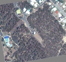
2
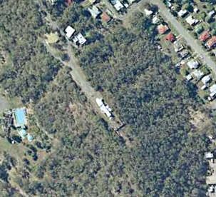
(2002)) and Google Earth Pro satellite images show the met-office was demolished and
replaced between 2003 and 2006 (Figure 1). Site diagrams show the Stevenson screen
relocated between 2004 and 2005 but metadata does not mention when a 60-litre Stevenson
screen replaced the former 230-litre one or when the current Almos AWS was commissioned.
Missing data from when thermometers were removed in 1993 to 2000 showed out-of-range
values were culled and that the AWS was probably replaced in late 2000.
The study aims to determine whether trajectory of the data reflect site and instruments
changes or changes in the climate.
x
Figure 1. The Gladstone Radar met-office on 17 May 2003 (left; portion of QAP5850057) and 4 January
2006 (Google Earth Pro satellite image). The Stevenson screen and AWS cabinet visible in the satellite
image near (x) was relocated from behind the office during the intervening period. Images are
comparably scaled and aligned. Trees up to 6 m in height surround the cleared area. The site was
reconfigured when the office was demolished in 2004.
2. The physical basis
2.1 Maximum temperature
Consistent with the First Law of thermodynamics, evaporation cools the local environment by
removing energy as latent heat at the rate of 2.45 MJ/kg of water evaporated, which at dryland
sites can’t exceed the rainfall (± 5%; dewfall may not be measured for example, neither is
runoff or drainage below the root zone).
As 1-mm rainfall = 1 kg/m2, evaporation of Gladstone Radar median rainfall (841 mm)
accounts for 2060 MJ/m2/yr of available net energy (the balance between incoming short-
wave solar radiation and long-wave emissions), which is 27.6% of average solar exposure
(7470 MJ/m2/yr) as estimated since January 1990 using satellite and albedo data. Assuming
that at annual timesteps cyclical gains and losses by the landscape (ground heat flux) cancel-
out, the remaining portion not used for evaporation, is advected to the local atmosphere as
sensible heat and is measured as maximum temperature (Tmax) by thermometers held 1.2 m
above the ground in a Stevenson screen. Thus the First Law theorem predicts that dry years
are warm and the drier it is the warmer it gets.
In the parlance of the statistical package R1, for a consistent well maintained site, dependence
of Tmax on rainfall (Tmax ~ rainfall) is likely to be statistically significant (Preg 0.05). However, if site control is poor or
1
https://www.r-project.org/3
observations are lackadaisical, significances and variation explained is less and in the extreme
case that Tmax is random to rainfall, data don’t reflect the weather and are not useful for
tracking trends and changes in the climate. Thus in keeping with the First Law theorem,
statistical significances of coefficients and variation explained objectively characterise data
fitness.
2.2 Minimum temperature
Minimum temperature (Tmin), which occurs in the early morning usually around dawn,
measures the balance between heat stored by the landscape the previous day and heat lost by
long-wave radiation to space overnight. Although affected by cloudiness/humidity, which
reduce emissions, and local factors such as inversions and cool-air drainage, a statistically
significant dependent relationship is expected between Tmin and Tmax.
To summarise, while rainfall (which also proxies cloudiness) directly reduces Tmax via the
water cycle (Figure 2(a)), rainfall’s relationship with Tmin may not be significant (Figure
2(b)). In contrast, the relationship between Tmin and Tmax (sometimes expressed as the
diurnal temperature range (DTR)) is expected to be linear and robust (i.e. significant
(Preg 0.05 (c) R 0.38
m
1m
500 1000 1500 500 1000 1500 27 28 29
84
Rainfall (mm) Tmax (oC)
Figure 2. Naïve relationships between Tmax and Tmin and rainfall, and Tmin and Tmax. Median rainfall
and average Tmax and Tmin are indicated by dotted lines. Values that appear to be out of range relative
to that year’s rainfall (or Tmax) are indicated. Tmin and rainfall are uncorrelated (Preg >0.05).
3. Statistical methods
3.1 Overview
As site and instrument changes occur in parallel with observations, trend and change is
confounded within the signal of interest. Stepwise analysis separates the confounded signals,
tests for changes in residuals and verifies they are associated with site changes. The aim is to
provide an unbiased explanation of the process, which is the evolution of temperature through
time.
The 3-stage approach involves:
(i) Exploratory data analysis tests the significance (Preg) and strength (R2adj) of
relationships between Tmax, Tmin and rainfall, and Tmin and Tmax using naïve linear
regression (Figure 2). However, only relationships that are statistically significant are
of interest (Figure 2(a) and Figure 2(c)).4
Linear regression partitions overall variation in temperature into that attributable to
the covariate (deterministic variation represented by the straight lines in Figure 2)
and the residual component, which although expected to be random, potentially
embed site-change and other systematic effects.
(ii) Re-scaled for convenience by adding grand-mean T, randomness of residuals is
evaluated using an objective statistical test of the hypothesis that mean-T is constant
(i.e. that rescaled residuals are homogeneous).
Permanent step-changes or (Sh)ifts in re-scaled residuals indicate the background
heat-ambience of the site or something related to the instrument changed
independently of the covariate. Detected step-changes are cross-referenced where
possible to metadata, historic site information and aerial photographs otherwise
statistical inference is the only evidence that data are not homogeneous. (If residuals
are random there are no inhomogeneities.)
(iii) Step-change analysis is verified using multiple linear regression of the T-covariate
relationship with step-change scenarios specified as category variables (viz. T ~ Shfactor
+ covariate).
Possible outcomes are: (a), Shfactor means are the same and interaction1 between
Shfactor and the covariate is not significant [segments are coincident, in which case
they are indexed the same and reanalysed]; (b), Shfactor means are different and
interaction is not significant [segmented responses to the covariate is the same (i.e.
lines are parallel) and the covariate-adjusted difference between segment means
measures the ‘true’ magnitude of the discontinuity]; (c) interaction is significant
[responses are not consistent; Shfactor specification is irrelevant or changepoints are
redundant (Shfactor changepoints don’t reflect the data)]; (d), T is random to the
covariate [observations are not consistent, don’t reflect the weather and can’t reflect
the climate].
Multiple linear regression residuals (i.e. data minus significant Shfactors and covariate effects)
are exported and examined for normality, equality of variance across categories,
independence (autocorrelation) and serial clustering. Trend of individual segments is checked
to assure the step-change model is appropriate.
3.2 Statistical tools
Sequential t-test analysis of regime shifts (STARS)2 is used for step-change analysis of both
raw-T and re-scaled residuals (https://www.beringclimate.noaa.gov/regimes/) and the R
packages3 Rcmdr and lsmeans are used for linear and multiple linear regression and to test
differences between segment means holding the covariate constant (at its median (rainfall) or
average (Tmax) level). Additional tests (normality, independence, clustering, Kruskall-Wallis
(non-parametric) 1-way analysis of variance on ranks) etc. are performed using the statistical
application PAST from the Natural History Museum, University of Oslo
(https://folk.uio.no/ohammer/past/). As data and statistical tools are in the public domain
analyses is fully replicable.
1
The R function lm is used to fit linear models (i.e. estimate coefficients from data and evaluate the overall
model fit); Type II analysis of variance (car package) conducts hypothesis tests on coefficients; a separate test
(of the form Tmax ~ Shfactor * covariate) evaluates equality of regression slopes while lsmeans tests differences
between segment means controlling for the covariate.
2
https://pdfs.semanticscholar.org/7746/6a6af18275339c2ef0bf4959e1c20b3b82cd.pdf
3
https://www.rcommander.com/; https://cran.r-project.org/web/packages/lsmeans/lsmeans.pdf5
3.3 Comparison of change scenarios
Multiple linear regression is used to compare Shfactor scenarios and whether documented site
changes (ShSite) are significant or if other changepoints better fit the data. While all
combinations are evaluated, the disciplined outcome is that segmented regressions are offset
and parallel (Section 3.1 (iii (b)). It’s possible for example, that the main site change was in
1991 when the AWS was installed; or in 1993, when manual observation ceased; or in 1993
and 2004 when the met-office was demolished (Figure 1). Alternatively, there was a Tmax
step-change in 2004 and a Tmax rainfall-residual step-change in 2001 (which is not cross-
referenced by available metadata; however, as the step-change aligns with cessation of
removing out of range values, it is likely the AWS was replaced and a 60-litre Stevenson
screen installed in place of the previous 230-litre one). Step-change scenarios that plausibly fit
Tmax data are shown in Figure 3.
M 1? 3
M 1? 3
h 0 99
h 0 99
is 20 s 1
is 20 s 1
04
04
20
20
m en ter
m en ter
de cre me
de scre me
O
O
th 91
th 91
s o
o
sm erm
sm erm
no 19
no 19
ol
ol
S
S
ShSite Tmax vs. rainfall ShSite1 Tmax vs. rainfall
AW
AW
2005 Prain 0.06 Prain 0.07
29 2005 29
1991 a
28 28 a
Temperature ( C)
27 a 27 b
o
1993
(a) 1983 1983 (b)
1960 1980 2000 500 1000 1500 1960 1980 2000 500 1000 1500
ShSite2 Tmax vs. rainfall ShMax2001 vs. 2004
2
2005 R 0.52
2009
29 29 2017
2001 2013
28 b 28 a
27 2003 a 27 2004 b
1993 a
(c) (d)
1960 1980 2000 500 1000 1500 1960 1980 2000 500 1000 1500
Rainfall (mm) Rainfall (mm)
Figure 3. Horizontal lines plausibly explain persistent changes in Tmax. Except for the 2001 shift in (d),
which was detected statistically using STARS; to illustrate possible scenarios, others were calculated
manually. Multiple linear regression tests if Tmax is correlated with rainfall overall and if differences in
median-rainfall adjusted means are the same (differences are indicated by letters beside each line). In all
cases interaction was not significant, which confirms that free-fit lines were parallel.
The same site changes potentially affect Tmin. In addition, there is a shift in Tmin vs. Tmax-
residuals in 1973, 1983 and 1999 (ShMinMaxRes) and first-round analysis found no
difference in segment means from 1973 to 1982 and 1999 to 2017 (thus regressions were
coincident). Another scenario results from combining those segments (ShMinMaxRes1).
There is also a shift in raw-Tmin in 1979, which could reflect the weather or something else.
Analysis sets out to construct a design-overlay for an experiment whose data are available but
‘treatments’ and when they were applied are unknown. It is important the problem is
approached without bias (i.e. all possibilities are considered) and that analysis is independent
and statistically disciplined (i.e. that covariate coefficients are significant, adjusted segment
means are different indicating lines are offset and interaction is not significant).
So the question is: which scenario best explains each dataset?
Scenario analyses are summarised in Table 1. For Tmax, the expected physical dependence of
Tmax on rainfall is not significant (P >0.05) for scenarios (ii) and (iii), which indicates
hypothesised step-changes are irrelevant (significance is reduced relative to (i), which is the
base-case). Although the covariate is significant for scenario (iv) the hypothesised change in
1993 is not (rainfall adjusted segment means pre- and post-1993 (to 2003) are the same.
Scenarios (v) and (vi) appear to be equivalent; however variation explained by Scenario (vi) is6
higher (51.7% vs. 43.4%), and the Akaike information criterion (AIC)1 (which measures the
relative quality of alternative models applied to the same dataset) is lower, indicating Scenario
(vi) is the better (more parsimonious) fit. (AIC is not given where factors and or the covariate
are not significant.)
Table 1. Multiple linear regression of Tmax and Tmin step-change scenarios. Non significance (ns) of the
covariate indicates lack of agreement between the statistical model and the First Law theorem.
Tmax vs. rainfall Change yearsSignificance Covariate AIC Covariate coefficient
(P) (R2adj)
(i) Tmax ~Rainfall na 0.02 100.43 -0.060oC/100 mm rainfall
(0.072)
(ii) ShSite 1991P7 skewed higher by 1973 and 1980 data (Figure 4 (b); Table 1, Tmin Case (iv)) as they were coincident they combine into a single category (Table 1, Tmin Case (v)). Second-round analysis (Figure 4 (c)) shows regressions are parallel and offset; Tmin increases 0.59oC/oCTmax and with Tmax held at its long-term average (27.6oC) the cumulative Tmin difference from the start of the record is 0.28oC. Furthermore, multiple linear regression residuals and individual data segments in Figure 4 (a) are untrending. Although data for 1960, 1974, 1983 and 2010 are likely outliers (but not excluded), the overall raw-Tmin trend of 0.16oC/decade (Punc
8
are normally distributed, independent and variance is random. Analysing raw data in the time-
domain (vs. the covariate-domain) is made difficult by confounding of site-change effects
with observations. Furthermore, it is necessary that the covariate is also accounted for so
apparent temperature changes are not due to sustained shifts in the covariate attributable to,
for example, the El Niño southern oscillation affecting rainfall. Multiple linear regression
removes covariate and step-change signals simultaneously, which provides an unbiased
assessment of the data-generating process.
4.3 Site and instrument changes
For a climate-warming (or cooling) argument to prevail it must be shown unequivocally that
trend or change is not biased by changes at the site between 1969 and 1992 and 2003 and
2006; installation and upgrading of weather radars and changes to the AWS and Stevenson
screens. If they are influential, such changes are detectable as a shift the ambient baseline
against which daily-T is measured, cooler or warmer depending on the nature of the change.
Removing the effect of causal covariates (rainfall and antecedent heat) exposes underlying
shifts in the baseline, which are detected objectively as non-climate related discontinuities.
The process outlined in Section 3 disaggregates the total signal into the deterministic portion
attributable to the covariate and that which is unexplained, including embedded
inhomogeneties and other systematic signals such as cycles and trends. Detecting those
objectively, re-entering them as categorical variables and evaluating their impacts using a
rules-based framework makes use of all the data, improves precision and reduces the
likelihood of not detecting trends and changes that exert a measurable impact on the processes
generating the data. Comparing scenarios statistically and objectively leads to a single
parsimonious outcome.
The abrupt Tmax step-change of 0.83oC in 2001, which is not rainfall-related is likely due to
commissioning of the current Almos AWS operating with a 60-litre Stevenson screen in
either 1999 or 2000. Likewise, since the start of the record in 1958, site changes in 1973,
1982 and 1999 caused Tmin to increase 0.28oC. Multiple linear regression assumptions are
not violated so the process is fully explained and as there is no residual trend, cycles or
inhomogeneties, there is no evidence that the climate has changed or warmed.

Figure 5. Aerial photographs show the met-office was enlarged and the area behind the building was
cleared and extended between November 1969 (left) and January 1992 (zoomed and cropped portions of
QAP204702 and QAP502722). WF44 radar was installed in on a lattice tower in May 1972 but other
changes and when they occurred are not detailed in site-summary metadata. (Photos are aligned at about
the same scale.)
9
5. Conclusions
Covariate analysis of temperature data is robust and rigorous and has been used to analyse
>200 long and medium-term datasets from across Australia. The most prevalent problem is
that poorly documented site and instrument changes result in spurious trends in naïvely-
analysed data. Analysis with causal covariates (rainfall in the case of Tmax and Tmax in the
case of Tmin) circumvents that observations are confounded with non-climate effects.
Analysis in the covariate domain also sidesteps common problems inherent in direct time-
series analysis such as incomplete data, outliers, data-fitness relative to statistical benchmarks
and autocorrelation, unequal variance and non-normality of residuals. Time series analysis
also provides no insights into the processes generating the data.
Sequential analysis is summarised thus:
   (i)     The strength of naïve relationships between temperature and covariates are
           assessed in the first instance and properties of residuals are evaluated graphically
           and statistically using appropriate tests.
   (ii)    With covariate effects removed, residuals are tested for inhomogeneties in the time
           domain. More than one scenario may be identified, which may or may not align
           with changes documented in metadata. Changepoints are specified using dummy
           or category variables added to the original dataset. Likewise for documented
           changes.
   (iii)   Multiple linear regression is used compare and contrast scenarios. There is only
           one outcome: with only significant factors included, individual regressions are
           offset (covariate adjusted differences are significant) and parallel (interaction is
           not significant thus slopes are homogeneous).
Post hoc testing examines residuals for unexplained systematic signals; data and residuals for
data-segments identified in step (ii) are examined separately for trend, outliers etc. Site
change effects are also verified using independent sources including aerial photographs and
satellite images, historical newspapers etc., documents in archives and metadata.
As multiple linear regression residuals embed no trend, step-changes or other systematic
signals it is concluded that the climate of Gladstone has not materially changed or warmed
since records commenced in 1958.

This research includes intellectual property that is copyright (©).

Preferred citation:
Johnston, Bill 2020. Climate of the Great Barrier Reef, Queensland. Part 1. Climate change at
Gladstone - a case-study. http://www.bomwatch.com.au/ 11 pp.
10
Appendix 1. Annual data for Gladstone Radar used in the study
Year Rain MaxAv MaxN MaxVar MinAv MinN MinVar
1958 955 27.95699 365 13.64702 18.43315 365 14.20266
1959 791.4 27.34712 365 11.75717 18.06904 365 13.20006
1960 770.2 27.55492 366 16.10248 17.53115 366 17.32456
1961 1070 27.44396 364 11.74098 17.65962 364 12.58682
1962 1257.5 27.4589 365 13.10424 18.25123 365 12.67712
1963 813.8 27.16329 365 11.85804 18.01315 365 13.57444
1964 718.5 27.93962 366 15.13303 18.68333 366 14.25986
1965 432.5 27.74603 365 14.34441 18.15425 365 12.77963
1966 807.8 27.31315 365 14.60895 17.97123 365 13.33618
1967 770.2 27.60438 365 16.39004 18.01589 365 12.072
1968 1041.2 27.89399 366 18.59969 18.11284 366 16.82918
1969 842.3 28.12 365 17.63869 18.70904 365 13.81896
1970 839.6 28.3074 365 10.72481 18.4811 365 14.1467
1971 1731.6 27.29534 365 13.65023 18.22959 365 14.41786
1972 662.5 27.46913 366 10.93069 17.93798 366 12.80855
1973 1418.2 27.9825 360 11.98434 19.19917 360 11.11947
1974 1205.2 26.95562 365 11.69028 17.81918 365 15.9065
1975 988.2 27.29096 365 11.40945 18.61836 365 11.91315
1976 970.4 27.47705 366 14.2404 18.33579 366 16.77288
1977 967.2 27.15808 365 11.7586 18.2874 365 16.05319
1978 962.2 27.03945 365 17.0191 18.15589 365 16.65461
1979 527.2 27.91452 365 12.62559 18.66329 365 13.56524
1980 840.8 28.0224 366 12.3744 19.04235 366 13.49785
1981 972.8 27.47253 364 14.45781 18.41456 364 16.35712
1982 538.2 27.45068 365 13.98295 18.36548 365 16.63227
1983 1441.8 26.68904 365 12.33548 18.77151 365 13.80155
1984 544.2 27 366 12.79342 18.5235 366 13.71073
1985 782.6 27.21315 365 15.48466 18.64575 365 16.00133
1986 1040.4 27.29425 365 14.53477 18.83699 365 13.2569
1987 698.4 27.63014 365 14.19601 18.67288 365 14.45264
1988 1083.2 27.80656 366 13.74187 18.82541 366 11.40541
1989 1087.1 26.85918 365 15.57511 18.00411 365 17.03787
1990 983.8 27.47699 365 17.96167 18.55808 365 17.68596
1991 841.6 27.87342 365 9.507067 18.87753 365 13.8185
1992 1135.4 27.32131 366 15.3602 18.64563 366 15.9798
1993 469.6 27.92708 336 10.30538 19.30564 337 9.211248
1994 648.6 27.8274 354 11.85327 18.57017 352 13.22335
1995 539.6 27.86698 321 16.42016 18.99818 330 16.10863
1996 996 27.33528 360 14.34936 18.72674 359 14.56548
1997 630.2 27.48157 331 11.63199 18.93012 332 12.17776
1998 738.2 28.03015 335 14.69121 19.19304 345 14.5292
1999 842.6 27.18547 344 10.61658 18.31268 347 11.78666
2000 845.4 27.04944 360 11.49008 17.92033 364 12.61909
2001 442.2 28.28 360 11.6201 18.62527 364 13.31859
2002 577.2 28.38778 360 14.614 18.71644 365 14.1111
2003 1166.7 27.78788 363 9.807974 18.74093 364 11.1459
2004 698.2 28.70274 365 11.43675 18.87198 364 16.14428
2005 705.2 29.3074 365 15.64629 19.45726 365 14.4252
2006 663.4 28.80164 365 14.02203 18.83178 365 12.79717
2007 792.2 28.15644 365 17.56741 18.68301 365 16.12724
2008 1127 27.79342 365 14.17254 18.44027 365 15.56901
2009 650.4 29.08599 364 9.65647 19.08849 365 12.41602
2010 1559.6 27.48187 364 10.70165 18.88548 365 13.61729
2011 734.4 27.81397 365 13.7495 18.15014 365 16.94569
2012 764 27.8306 366 16.61281 18.37486 366 14.91668
2013 1446.4 28.33205 365 14.81114 18.94423 364 11.1360811 2014 941.4 28.17088 364 12.137 18.82082 365 14.01753 2015 685.2 28.5843 363 12.7284 18.85234 363 14.2793 2016 951.6 28.60904 354 15.06949 19.39831 356 13.03081 2017 983.2 28.82473 364 10.41256 19.54278 360 12.27505
You can also read