Co-localization in Real-World Images
←
→
Page content transcription
If your browser does not render page correctly, please read the page content below
Co-localization in Real-World Images

                     Kevin Tang1     Armand Joulin1       Li-Jia Li2                           Li Fei-Fei1
                1                                                                           2
                  Computer Science Department, Stanford University                            Yahoo! Research
                 {kdtang,ajoulin,feifeili}@cs.stanford.edu                         lijiali@yahoo-inc.com

                        Abstract

   In this paper, we tackle the problem of co-localization in
real-world images. Co-localization is the problem of simul-
taneously localizing (with bounding boxes) objects of the
same class across a set of distinct images. Although similar
problems such as co-segmentation and weakly supervised
localization have been previously studied, we focus on be-
ing able to perform co-localization in real-world settings,
which are typically characterized by large amounts of intra-
class variation, inter-class diversity, and annotation noise.
To address these issues, we present a joint image-box for-
mulation for solving the co-localization problem, and show
how it can be relaxed to a convex quadratic program which
can be efficiently solved. We perform an extensive eval-            Figure 1. The co-localization problem in real-world images. In
uation of our method compared to previous state-of-the-             this instance, the goal is to localize the airplane within each im-
art approaches on the challenging PASCAL VOC 2007 and               age. Because these images were collected from the Internet, some
Object Discovery datasets. In addition, we also present a           images do not actually contain an airplane.
large-scale study of co-localization on ImageNet, involv-
                                                                    notation noise [24, 30, 31], most previous works related to
ing ground-truth annotations for 3,624 classes and approx-
                                                                    co-localization have assumed clean labels, which is not a
imately 1 million images.
                                                                    realistic assumption in many real-world settings where we
                                                                    have to analyze large numbers of Internet images or dis-
                                                                    cover objects with roaming robots. Our aim is therefore to
1. Introduction                                                     overcome the challenges posed by noisy images and object
   Object detection and localization has long been a cor-           variability.
nerstone problem in computer vision. Given the variabil-                We propose a formulation for co-localization that com-
ity of objects and clutter in images, this is a highly chal-        bines an image model and a box model into a joint opti-
lenging problem. Most state-of-the-art methods require ex-          mization problem. Our image model addresses the problem
tensive guidance in training, using large numbers of im-            of annotation noise by identifying incorrectly annotated im-
ages with human-annotated bounding boxes [11, 28]. Re-              ages in the set, while our box model addresses the prob-
cent works have begun to explore weakly-supervised frame-           lem of object variability by localizing the common object
works [9, 14, 21, 22, 27, 29], where labels are only given          in each image using rich correspondence information. The
at the image level. Inspired by these works, we focus on            joint image-box formulation allows the image model to ben-
the problem of unsupervised object detection through co-            efit from localized box information, and the box model to
localization, which further relaxes the need for annotations        benefit by avoiding incorrectly annotated images.
by only requiring a set of images that each contain some                To illustrate the effectiveness of our method, we present
common object we would like to localize.                            results on three challenging, real-world datasets that are
   We tackle co-localization in real-world settings where           representative of the difficulties of intra-class variation,
the objects display a large degree of variability, and worse,       inter-class diversity, and annotation noise present in real-
the labels at the image level can be noisy (see Figure 1).          world images. We outperform previous state-of-the-art ap-
Although recent works have tried to explicitly deal with an-        proaches on standard datasets, and also show how the joint

                                                                1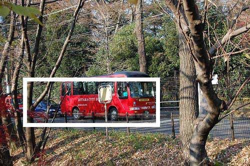
image-box model is better at detecting incorrectly anno-
tated images. Finally, we present a large-scale study of co-
localization on ImageNet [8], involving ground-truth anno-                                        Original Images
tations for 3,624 classes and 939,542 images. The largest
previous study of co-segmentation on ImageNet consisted
of ground-truth annotations for 446 classes and 4,460 im-
ages [18].                                                                                   Candidate Bounding Boxes

                                                                                 Box Model                              Image Model
2. Related Work
    Co-localization shares the same type of input as co-
segmentation [15–18,24,33], where we must find a common
object within a set of images. However, instead of segmen-
tations, we seek to localize objects with bounding boxes.
Considering boxes allows us to greatly decrease the num-
                                                                                              Joint Image-Box Model
ber of variables in our problem, as we label boxes instead of
pixels. It also allows us to extract rich features from within
the boxes to compare across images, which has shown to be
very helpful for detection [32].
    Co-localization shares the same type of output as weakly                                    Co-localized Images

supervised localization [9, 21, 22, 27], where we draw
bounding boxes around objects without any strong super-             Figure 2. Given a set of images, we start by generating a set of
vision. The key difference is that in co-localization we            candidate boxes independently for each image. Then, our joint
                                                                    image-box model is able to simultaneously identify the noisy im-
have a more relaxed scenario, where we do not know what
                                                                    ages and select the box from each clean image that contains the
the object contained in our set of images is, and are not
                                                                    common object, resulting in a set of co-localized images. Previ-
given negative images for which we know do not contain              ous work considers only the box model [9].
our object. Most similar is [9], which generates candidate
bounding boxes and tries to select the correct box within           is to simultaneously identify the noisy images and localize
each image using a conditional random field. Object co-             the common object in the clean images.
detection [3] also shares similarities, but is given additional         An overview of our approach is given in Figure 2. We
bounding box and correspondence annotations.                        start by generating a set of candidate boxes for each image
    Although co-localization shares similarities with both          that could potentially contain an object. Then, we formulate
co-segmentation and weakly supervised localization, an im-          an image model for selecting the clean images, and a box
portant and new difficulty we address in this paper is the          model for selecting the box in each image that contains an
problem of noisy annotations, which has recently been con-          instance of the common object. We denote the boxes that
sidered [24, 30, 31]. Most similar is [24], where the authors       contain an instance of the common object as positive boxes,
utilize dense correspondences to ignore incorrect images.           and the ones that don’t as negative boxes.
We combine an image model that detects incorrectly anno-                Combining the two models into a joint formulation, we
tated images with a box model that localizes the common             allow the image model to prevent the box model from be-
object, which sets us apart from previous work. The ob-             ing adversely affected by boxes in noisy images, and allow
jective functions in our models are inspired by works from          the box model to help the image model determine noisy im-
outlier detection [13], image segmentation [26], and dis-           ages based on localized information in the images. Similar
criminative clustering [2, 15, 34]. Previous works have con-        approaches have been considered [9], but only using a box
sidered combining object detection with image classifica-           model and only in the context of clean images.
tion [11, 28], but only in supervised scenarios.
                                                                    3.1. Generating candidate boxes
3. Our Approach
                                                                       We use the measure of objectness [1], but any method
    Given a set of n images I = {I1 , I2 , . . . , In }, our goal   that is able to generate a set of candidate regions can be
is to localize the common object in each image. In addition,        used [5, 32]. The objectness measure works by combining
we also consider the fact that due to noise in the process of       multiple image cues such as multi-scale saliency, color con-
collecting this set, some images may not contain the com-           trast, edge density, and superpixel straddling to generate a
mon object. We denote these as noisy images, as opposed to          set of candidate regions as well as scores associated with
clean images, which contain the common object. Our goal             each region that denote the probability a generic object is
z1,1 = 1               is only one positive box, and in each noisy image there are
                 v1 = 1                                                    no positive boxes, we define a constraint that relates the two
                                                    z1,2 = 0               sets of variables:
                                                                                                        m
                                                                                                        X
   Image Model

                                                    z2,1 = 0                                 ∀Ij ∈ I,         zj,k = vj .            (1)

                                                               Box Model
                 v2 = 1                                                                                 k=1

                                                    z2,2 = 1               This constraint is also illustrated in Figure 3, where we
                                                                           show the relationship between image and box variables.
                                                    z3,1 = 0
                 v3 = 0                                                    3.3. Model formulation
                                                    z3,2 = 0                  We begin by introducing and motivating the terms in our
                                                                           objective function that enable us to jointly identify noisy
                                                                           images and select the positive box from each clean image.
Figure 3. The variables v in the image model relate to the variables
z in the box model through constraints that ensure noisy images            Box prior. We introduce a prior for each box that repre-
(red) do not select any boxes, while clean images (green) select a         sents our belief that the box is positive. We compute an
single box as the postive box.                                             off-the-shelf saliency map for each image [6, 23], and for
                                                                           each box we compute the average saliency within the box,
present in the region. Examples of candidate boxes gener-                  weighted by the size of the box, and stack these values into
ated by objectness can be seen in Figure 2.                                the nb dimensional vector mbox to obtain a linear term that
   Using the objectness measure, for each image Ij ∈                       penalizes less salient boxes:
I, we generate a set of m candidate boxes Bj =
{bj,1 , bj,2 , . . . , bj,m }, ordered by their objectness score.                         fP box (z) = −z T log(mbox ).              (2)
3.2. Model setup                                                           Although objectness also provides scores for each box, we
   Given a set of images I and a set of boxes Bj for each                  found that the saliency measure used in objectness is dated
image Ij ∈ I, our goal is to jointly determine the noisy                   and does not work as well.
images and select the positive box from each clean image.
                                                                           Image prior. We introduce a prior for each image that
To simplify notation, we define the set of all boxes as B =
                                                                           represents our belief that the image is a clean image. For
B1 ∪ B2 . . . ∪ Bn and nb = nm the total number of boxes.
                                                                           each image, we compute the χ2 distance, defined further be-
Feature representation. For each box bk ∈ B, we com-                       low, from the image feature to the average image feature in
pute a feature representation of the box as xbox  ∈ Rd , and               the set, and stack these values into the n dimensional vector
                                             k
stack the feature vectors to form a feature matrix Xbox ∈                  mim to obtain a linear term that penalizes outlier images:
Rnb ×d . Similarly for each image Ij ∈ I, we compute a fea-
ture representation of the image as xim     d                                                  fP im (v) = v T mim .                 (3)
                                     j ∈ R , and stack the
feature vectors to form a feature matrix Xim ∈ Rn×d . We
                                                                           We experimented with several measures for outlier detec-
densely extract SIFT features [20] every 4 pixels and vector
                                                                           tion [13], but found that this simple distance worked well.
quantize each descriptor into a 1,000 word codebook. For
each box, we pool the SIFT features within the box using                   Box similarity. We encourage boxes with similar appear-
1 × 1 and 3 × 3 SPM pooling regions [19], and for each im-                 ances to have the same label through a similarity matrix
age, we use the same pooling regions over the entire image                 based on the box feature described above. Since this fea-
to generate a d = 10, 000 dimensional feature descriptor for               ture is a histogram, we compute a nb × nb similarity matrix
each box and each image.                                                   S based on the χ2 -distance:
Optimization variables. We associate with each image                                                  d
                                                                                                                            !
                                                                                                      X (xbox   box 2
                                                                                                          ik − xjk )
Ij ∈ I a binary label variable vj , which is equal to 1 if Ij                        Sij = exp −γ                               ,    (4)
is a clean image and 0 otherwise. Similarly, we associate                                             k=1
                                                                                                               xbox   box
                                                                                                                ik + xjk
with each box bj,k ∈ Bj a binary label variable zj,k , which
                                                                                               1
is equal to 1 if bj,k is a positive box and 0 otherwise. We                where γ = (10d)− 2 . We set the similarity of boxes from
denote by v, the n dimensional vector v = (v1 , . . . , vn )T              the same image to be 0. We then compute the normalized
                                                                                                            1     1
and by z the nb dimensional vector obtained by stacking the                Laplacian matrix Lbox = I − D− 2 SD− 2 , where D is the
zj,k . Making the assumption that in each clean image there                diagonal matrix composed of the row sums of S, resulting
in a quadratic term that encourages the selection of similar     Image discriminability. Similar to the box discriminabil-
boxes:                                                           ity term, we also employ a discriminative objective to en-
                                                                 sure that the features of the clean images should be easily
                   fSbox (z) = z T Lbox z.                (5)    linearly separable from noisy images. Replacing the box
                                                                 features in Equation 7 with image features, we can similarly
This choice is motivated by the work of Shi and Malik [26],      substitute the solutions for w and c to obtain:
who have shown that considering the second smallest eigen-
vector of a normalized Laplacian matrix leads to clustering                         fDim (v) = v T Aim v,                   (9)
z along the graph defined by the similarity matrix, lead-
                                                                 where Aim is defined in the same way as Abox , replacing
ing to Normalized Cuts when used for image segmentation.
                                                                 box features with image features.
Furthermore, Belkin and Niyogi [4] have shown that min-
imizing Equation 5 under linear constraints results in an        Joint formulation. Combining the terms presented
equivalent problem. The similarity term can be interpreted       above, we obtain the following optimization problem:
as a a generative term that seeks to select boxes that cluster
well together.                                                      minimize      z T (Lbox + µAbox )z − z T λ log(mbox )
                                                                        z,v

Image similarity. We also encourage images with simi-                             + α(v T (Lim + µAim )v + v T λmim )
lar appearances to have the same label through a similarity         subject to    v ∈ {0, 1}, z ∈ {0, 1}
matrix based on the image feature described above. Re-                                     Xm
placing the box features with image features in Equation 4,                       ∀Ij ∈ I,      zj,k = vj
we compute a n × n similarity matrix and subsequently the                                  k=1
normalized Laplacian matrix Lim to obtain a quadratic term                               n
                                                                                         X
that encourages the selection of similar images:                                  K0 ≤         vi ,                      (10)
                                                                                         i=1
                    fSim (v) = v T Lim v.                 (6)    where the constraints in the formulation ensure that only a
                                                                 single box is selected in clean images, and none in noisy
Box discriminability. Discriminative learning techniques         images. Using the constant K0 , we can avoid trivial solu-
such as the support vector machine and ridge regression          tions and incorporate an estimate of noise by allowing noisy
have been widely used within the computer vision commu-          images to not contain boxes. This prevents the boxes in
nity to obtain state-of-the-art performance on many super-       the noisy images from adversely affecting the box similar-
vised problems. We can take advantage of these methods           ity and discriminability terms.
even in our unsupervised scenario, where we do not know              The parameter µ controls the tradeoff between the
the labels of our boxes [2, 34]. Following [15], we consider     quadratic terms, the parameter λ controls the tradeoff be-
the ridge regression objective function for our boxes:           tween the linear and quadratic terms, and the parameter α
                                                                 controls the tradeoff between the image and box models.
              n m
          1 XX                           κ                       Since the matrices Lbox , Abox , Lim , and Aim are each pos-
   min            ||zj,k − wxbox      2        2
                             j,k − c||2 + ||w||2 ,        (7)
   w∈Rd , nb                             d                       itive semi-definite, the objective function is convex.
             j=1 k=1
    c∈R
                                                                 Convex relaxation. In Equation 10, we obtain a standard
where w is the d dimensional weight vector of the classifier,    boolean constrained quadratic program. The only sources
and c is the bias. The choice of ridge regression over other     of non-convexity in this problem are the boolean constraints
discriminative cost functions is motivated by the fact that      on v and z. We relax the boolean constraints to continuous,
the ridge regression problem has a closed form solution for      linear constraints, allowing v and z to take any value be-
the weights w and bias c, leading to a quadratic function in     tween 0 and 1. This becomes a convex optimization prob-
the box labels [2]:                                              lem and can be solved efficiently using standard methods.
                                                                    Given the solution to the quadratic program, we recon-
                   fDbox (z) = z T Abox z,                (8)    struct the solution to the original boolean constrained prob-
                                                                 lem by thresholding the values of v to obtain the noisy im-
where Abox = n1b (Πnb (Inb − Xbox (Xbox      T
                                                 Πnb Xbox +      ages, and simply taking the box from each clean image with
       −1 T                              1      T
nb κI) Xbox )Πnb ) and Πnb = Inb − nb 1nb 1nb is the cen-        the highest value of z.
tering projection matrix. We know also that Abox is a pos-
itive semi-definite matrix [12]. This quadratic term allows      4. Results
us to utilize a discriminative objective function to penalize
                                                                    We perform experiments on three challenging datasets,
the selection of boxes whose features are not easily linearly
                                                                 the PASCAL VOC 2007 dataset [10], the Object Dis-
separable from the other boxes.
aeroplane bicycle boat bus horse motorbike
Method left right left right left right left right left right left right Average
Our Method (prior) 13.95 20.51 10.42 8.00 2.27 6.98 9.52 13.04 12.50 13.04 17.95 23.53 12.64
Our Method (prior+similarity) 39.53 35.90 25.00 24.00 0.00 2.33 23.81 34.78 37.50 43.48 48.72 58.82 31.16
Our Method (full) 41.86 51.28 25.00 24.00 11.36 11.63 38.10 56.52 43.75 52.17 51.28 64.71 39.31
Table 1. CorLoc results for various combinations of terms in our box model on PASCAL07-6x2.
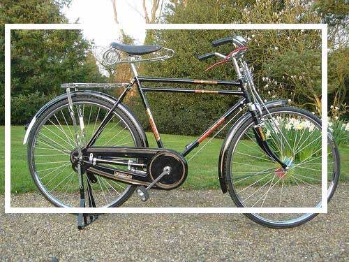
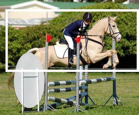
Figure 4. Example co-localization results on PASCAL07-6x2. Each column contains images from the same class/viewpoint combination.
Method Average CorLoc Method Airplane Car Horse Average CorLoc
Russell et al. [25] 22 Kim et al. [17] 21.95 0 16.13 12.69
Chum and Zisserman [7] 33 Joulin et al. [15] 32.93 66.29 54.84 51.35
Deselaers et al. [9] 37 Joulin et al. [16] 57.32 64.04 52.69 58.02
Our Method 39 Rubinstein et al. [24] 74.39 87.64 63.44 75.16
Our Method 71.95 93.26 64.52 76.58
Table 2. CorLoc results compared to previous methods on
PASCAL07-6x2. Table 3. CorLoc results on the 100 image subset of the Object
Discovery dataset.
covery dataset [24], and ImageNet [8]. Following previ-
ous works in weakly supervised localization [9], we use train+val dataset from the left and right aspect each. Each
the CorLoc evaluation metric, defined as the percentage of the 12 class/viewpoint combinations contains between 21
of images correctly localized according to the PASCAL- and 50 images for a total of 463 images.
area(B ∩B )
criterion: area(Bpp ∪Bgt
gt )
> 0.5, where Bp is the predicted In Table 1, we analyze each component of our box
box and Bgt is the ground-truth box. All CorLoc results are model by removing various terms in the objective. As ex-
given in percentages. pected, we see that results using stripped down versions of
our model do not perform as well. In Table 2, we show
4.1. Implementation details and runtime how our full method outperforms previous methods for co-
We set the parameters of our method to be µ = 0.6, localization that do not utilize negative images. In addi-
λ = 0.001, and α = 1, and tweaked them slightly for each tion, our method does not incorporate dataset-specific as-
dataset. We set κ = 0.01 in the ridge regression objective. pect ratio priors for selecting boxes. In Figure 4, we show
Because there are no noisy images for PASCAL and Ima- example visualizations of our co-localization method for
geNet, we fix the value of K0 = n for these datasets. For PASCAL07-6x2. In the bus images, our model is able to
the Object Discovery dataset, we set K0 = 0.8n. We use co-localize instances in the background, even when other
10 objectness boxes for ImageNet, and 20 objectness boxes objects are more salient. In the bicycle and motorbike im-
for the other datasets. ages, we see how our model is able to co-localize instances
After computing candidate object boxes using objectness over a variety of natural and man-made background scenes.
and densely extracting SIFT features, we are able to co-
localize a set of 100 images with 10 boxes per image in 4.3. Object Discovery dataset
less than 1 minute on a single machine using code written The Object Discovery dataset [24] was collected by au-
in Python and a quadratic program solver written in C++. tomatically downloading images using the Bing API using
queries for airplane, car, and horse, resulting in noisy im-
4.2. PASCAL VOC 2007
ages that may not contain the query. Introduced as a dataset
Following the experimental setup defined in [9], we eval- for co-segmentation, we convert the ground-truth segmen-
uate our method on the PASCAL07-6x2 subset to compare tations and results from previous methods to localization
to previous methods for co-localization. This subset con- boxes by drawing tight bounding boxes around the segmen-
sists of all images from 6 classes (aeroplane, bicycle, boat, tations. We use the 100 image subset [24] to enable com-
bus, horse, and motorbike) of the PASCAL VOC 2007 [10] parisons to previous state-of-the-art co-segmentation meth-
(a)                                                                                                 (b)

Figure 5. (a) Example co-localization results on the Object Discovery dataset, with every three columns belonging to the same class; (b)
Images from the airplane class that were incorrectly localized.
                                  Airplane                                                           Car                                                          Horse
              1                                                            1                                                                  1
                                                                                                                                                                                 Image model
            0.8                                                          0.8                                                                0.8                                  Image−Box model
            0.6                                                          0.6                                                                0.6
Precision

                                                             Precision

                                                                                                                                Precision
            0.4                                                          0.4                                                                0.4

            0.2                                                          0.2                                                                0.2

              0                                                            0                                                                  0
                  0   0.2   0.4              0.6   0.8   1                     0   0.2         0.4            0.6   0.8     1                     0   0.2   0.4            0.6         0.8         1
                                    Recall                                                           Recall                                                       Recall

Figure 6. Precision-recall curves illustrating the effectiveness of our image-box model (blue) compared to the image model (pink) at
identifying noisy images on the Object Discovery dataset. The joint optimization problem allows the box model to help correct errors
made by the image model.

ods. CorLoc results are given in Table 3, and example co-                                                                  Method                           Average CorLoc
localization results are visualized in Figure 5(a). From the                                                        Top objectness box [1]                         37.42
                                                                                                                         Our Method                                53.20
visualizations, we see how our model is able to handle intra-
class variation, being able to co-localize instances of each                                               Table 4. CorLoc results on ImageNet evaluated using ground-truth
object class from a wide range of viewpoints, locations, and                                               annotations for 3,624 classes and 939,542 images.
background scenes. This is in part due to our quadratic
terms, which consider the relationships between all pairs of                                               4.4. ImageNet
images and boxes, whereas previous methods like [24] rely
                                                                                                               ImageNet [8] is a large-scale ontology of images or-
on sparse image connectivity for computational efficiency.
                                                                                                           ganized according to the WordNet hierarchy. Each node
   We see that our method outperforms previous methods                                                     of the hierarchy is depicted by hundreds and thousands of
in all cases except for the airplane class. In Figure 5(b), we                                             images. We perform a large-scale evaluation of our co-
see that since our method localizes objects based on boxes                                                 localization method on ImageNet by co-localizing all im-
instead of segmentations [24], the airplane tail is some-                                                  ages with ground-truth bounding box annotations, resulting
times excluded from the box, as including the tail would                                                   in a total of 3,624 classes and 939,542 images. A similar
also include large areas of the background. This causes our                                                large-scale segmentation experiment [18] only considered
method to fail in these images due to the non-convex shape                                                 ground-truth annotations in 446 classes and 4,460 images.
of the airplane and the height of the tail.                                                                At this scale, the visual variability of images is unprece-
Detecting noisy images. We also quantitatively measure                                                     dented in comparison to previous datasets, causing methods
the ability of our joint image-box model to identify noisy                                                 specifically tuned to certain datasets to work poorly.
images. Because the solution to the quadratic program gives                                                    Due to the scale of ImageNet and lack of code available
continuous values for the image variables v, we can inter-                                                 for previous methods, we compare our method to the high-
pret the values as a detection score for each image and plot                                               est scoring objectness box [1], which gives a strong baseline
precision-recall curves that measure our ability to correctly                                              for generic object detection. To ensure fair comparisons,
detect noisy images, as shown in Figure 6. To make com-                                                    we use the objectness score as the box prior for our model
parisons fair, we compare using the best parameters for the                                                in these experiments, with CorLoc results shown in Table 4
image model alone, and the best parameters for our joint                                                   and visualizations for 104 diverse classes in Figure 7.
image-box model. By jointly optimizing over both image                                                     Box selection. In Figure 8(a), we show the distribution
and box models, we see how the box model can correct er-                                                   over objectness boxes that our method selects. The boxes
rors made by the image model by forcing images that have                                                   are ordered by decreasing objectness score, so objectness
good box similarity and discriminability to be clean, even if                                              simply selects the first box in every image. By consider-
the image model believes them to be noisy.                                                                 ing box similarity and discriminability between images, our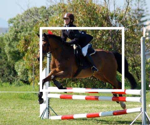
Figure 7. Example co-localization results on ImageNet. Each image belongs to a different class, resulting in a total of 104 classes ranging
from lady bug to metronome. White boxes are localizations from our method, green boxes are ground-truth localizations.
                                                                                                6
method identifies boxes that may not have very high object-                                10                                                  70

ness score, but are more likely to be the common object.                                                                   CorLoc Percentage
                                                                        Number of Images

                                                                                                                                               60
Effect of ImageNet node height. We also evaluate the                                            5
                                                                                           10
performance of our method on different node heights in Im-
                                                                                                                                               50
ageNet in Figure 8(b). Here, a height of 1 is a leaf node,
and larger values result in more generic object classes. We                                10
                                                                                                4
                                                                                                                                               40
see that our method seems to perfom better as we go up the                                          1 2 3 4 5 6 7 8 9 10                            1 2 3 4 5 6 7 8 9 10
                                                                                                          Box Index                                       Node Height
ImageNet hierarchy. This could be because generic objects                                                 (a)                                             (b)
have more images, and thus our method has more examples
to leverage in the box similarity and discriminability terms.           Figure 8. (a) Boxes selected by our method on ImageNet, ordered
CorLoc difference between methods. In Figure 9, we                      by descending objectness score; (b) CorLoc performance of our
show the CorLoc difference between our method and ob-                   method separated into differing node heights of ImageNet.
jectness for all 3,624 classes. From the best CorLoc differ-
ences, we find that our method performs much better than                joint optimization problem. Our formulation is able to ac-
objectness on large rooms and objects, which is probably                count for noisy images with incorrect annotations. We per-
because objectness tries to select individual objects or ob-            formed an extensive evaluation of our method on standard
ject parts within these large scenes, whereas our model is              datasets, and also performed a large-scale evaluation using
able to understand that the individual objects are not simi-            ground-truth annotations for 3,624 classes from ImageNet.
lar, and select the scene or object as a whole.                            For future work, we would like to extend our model to
                                                                        the pixel level for tasks such as co-segmentation, and to han-
5. Conclusion                                                           dle multiple instances of objects.
    In this paper, we introduce a method for co-localization            Acknowledgments. We especially thank V. Ferrari for
in real-world images that combines terms for the prior, sim-            helpful comments, suggestions, and discussions. We also
ilarity, and discriminability of both images and boxes into a           thank N. Liu for implementation help, A. Alahi, J. Johnson,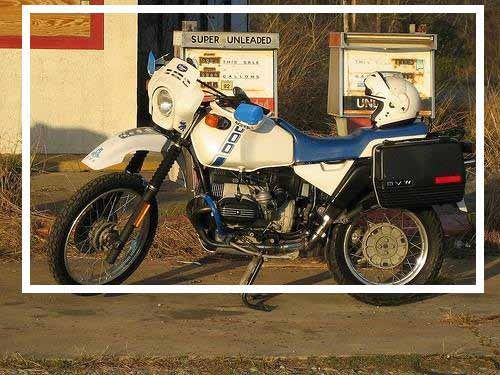
37. Mammoth
                                                                              [13] V. J. Hodge and J. Austin. A survey of outlier detection
                          407. Blender                                             methodologies. AI Rev., 22(2):85–126, 2004. 2, 3
                                         1146. Cat                            [14] A. Joulin and F. Bach. A convex relaxation for weakly su-
                                                              2422. Dolphin
                                                                                   pervised classifiers. In ICML, 2012. 1
                                                                              [15] A. Joulin, F. Bach, and J. Ponce. Discriminative clustering
                                                                                   for image co-segmentation. In CVPR, 2010. 2, 4, 5
                                                                              [16] A. Joulin, F. Bach, and J. Ponce. Multi-class cosegmentation.
                                                                                   In CVPR, 2012. 2, 5
                                                                              [17] G. Kim, E. P. Xing, L. Fei-Fei, and T. Kanade. Distributed
                                                     3612. Ball
                                                                                   cosegmentation via submodular optimization on anisotropic
                                                                                   diffusion. In ICCV, 2011. 2, 5
                                                                              [18] D. Küttel, M. Guillaumin, and V. Ferrari. Segmentation
                                                                                   propagation in imagenet. In ECCV, 2012. 2, 6
                                                                              [19] S. Lazebnik, C. Schmid, and J. Ponce. Beyond bags of
                                                                                   features: Spatial pyramid matching for recognizing natural
                                                                                   scene categories. In CVPR, 2006. 3
Figure 9. CorLoc difference between our method and objectness
                                                                              [20] D. G. Lowe. Distinctive image features from scale-invariant
on all 3,624 classes from ImageNet that we evaluate on.
                                                                                   keypoints. IJCV, 60(2):91–110, 2004. 3
O. Russakovsky, V. Ramanathan for paper comments. This                        [21] M. H. Nguyen, L. Torresani, F. de la Torre, and C. Rother.
research is partially supported by an ONR MURI grant, the                          Weakly supervised discriminative localization and classifi-
                                                                                   cation: a joint learning process. In ICCV, 2009. 1, 2
DARPA Mind’s Eye grant, the Yahoo! FREP, and a NSF
                                                                              [22] M. Pandey and S. Lazebnik. Scene recognition and weakly
GRFP under grant no. DGE-114747 (to K.T.).
                                                                                   supervised object localization with deformable part-based
                                                                                   models. In ICCV, 2011. 1, 2
References                                                                    [23] F. Perazzi, P. Krähenbühl, Y. Pritch, and A. Hornung.
 [1] B. Alexe, T. Deselaers, and V. Ferrari. Measuring the object-                 Saliency filters: Contrast based filtering for salient region
     ness of image windows. IEEE T-PAMI, 34(11):2189–2202,                         detection. In CVPR, 2012. 3
     2012. 2, 6                                                               [24] M. Rubinstein, A. Joulin, J. Kopf, and C. Liu. Unsupervised
 [2] F. Bach and Z. Harchaoui. Diffrac: a discriminative and flex-                 joint object discovery and segmentation in internet images.
     ible framework for clustering. In NIPS, 2007. 2, 4                            CVPR, 2013. 1, 2, 5, 6
 [3] S. Y. Bao, Y. Xiang, and S. Savarese. Object co-detection. In            [25] B. C. Russell, A. A. Efros, J. Sivic, W. T. Freeman, and
     ECCV, 2012. 2                                                                 A. Zisserman. Using multiple segmentations to discover ob-
 [4] M. Belkin and P. Niyogi. Laplacian eigenmaps for dimen-                       jects and their extent in image collections. In CVPR, 2006.
     sionality reduction and data representation. Neural compu-                    5
     tation, 15(6):1373–1396, 2003. 4                                         [26] J. Shi and J. Malik. Normalized cuts and image segmenta-
 [5] J. Carreira and C. Sminchisescu. Constrained parametric                       tion. IEEE T-PAMI, 22(8):888–905, 2000. 2, 4
     min-cuts for automatic object segmentation. In CVPR, 2010.               [27] P. Siva, C. Russell, T. Xiang, and L. de Agapito. Looking
     2                                                                             beyond the image: Unsupervised learning for object saliency
                                                                                   and detection. In CVPR, 2013. 1, 2
 [6] M.-M. Cheng, G.-X. Zhang, N. J. Mitra, X. Huang, and S.-
     M. Hu. Global contrast based salient region detection. In                [28] Z. Song, Q. Chen, Z. Huang, Y. Hua, and S. Yan. Contex-
     CVPR, 2011. 3                                                                 tualizing object detection and classification. In CVPR, 2011.
                                                                                   1, 2
 [7] O. Chum and A. Zisserman. An exemplar model for learning
                                                                              [29] K. Tang, V. Ramanathan, L. Fei-Fei, and D. Koller. Shifting
     object classes. In CVPR, 2007. 5
                                                                                   weights: Adapting object detectors from image to video. In
 [8] J. Deng, W. Dong, R. Socher, L.-J. Li, K. Li, and L. Fei-Fei.
                                                                                   NIPS, 2012. 1
     ImageNet: A Large-Scale Hierarchical Image Database. In
                                                                              [30] K. Tang, R. Sukthankar, J. Yagnik, and L. Fei-Fei. Discrimi-
     CVPR, 2009. 2, 5, 6
                                                                                   native segment annotation in weakly labeled video. In CVPR,
 [9] T. Deselaers, B. Alexe, and V. Ferrari. Weakly supervised
                                                                                   2013. 1, 2
     localization and learning with generic knowledge. IJCV,
                                                                              [31] A. Vahdat and G. Mori. Handling uncertain tags in visual
     100(3):275–293, 2012. 1, 2, 5
                                                                                   recognition. In ICCV, 2013. 1, 2
[10] M. Everingham, L. Van Gool, C. K. I. Williams, J. Winn, and
                                                                              [32] K. E. A. van de Sande, J. R. R. Uijlings, T. Gevers, and
     A. Zisserman. The PASCAL Visual Object Classes Chal-
                                                                                   A. W. M. Smeulders. Segmentation as selective search for
     lenge 2007 (VOC2007) Results. 4, 5
                                                                                   object recognition. In ICCV, 2011. 2
[11] H. Harzallah, F. Jurie, and C. Schmid. Combining efficient
                                                                              [33] S. Vicente, C. Rother, and V. Kolmogorov. Object coseg-
     object localization and image classification. In ICCV, 2009.
                                                                                   mentation. In CVPR, 2011. 2
     1, 2
                                                                              [34] L. Xu, J. Neufeld, B. Larson, and D. Schuurmans. Maximum
[12] T. Hastie, R. Tibshirani, and J. Friedman. The Elements of
                                                                                   margin clustering. In NIPS, 2004. 2, 4
     Statistical Learning. Springer-Verlag, 2001. 4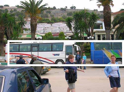
You can also read