Comment on Glenn Shafer's "Testing by betting" - arXiv
←
→
Page content transcription
If your browser does not render page correctly, please read the page content below
Comment on Glenn Shafer’s “Testing by betting”
                                                                            Vladimir Vovk∗
arXiv:2009.08933v2 [stat.ME] 6 May 2021

                                                                             May 7, 2021

                                                                                Abstract
                                                   This note is my comment on Glenn Shafer’s discussion paper “Testing
                                                by betting” [16], together with two online appendices comparing p-values
                                                and betting scores.
                                                The version of this note at http://alrw.net/e (Working Paper 8) is
                                                updated most often.

                                          Main comment
                                          Glenn Shafer’s paper is a powerful appeal for a wider use of betting ideas and
                                          intuitions in statistics. He admits that p-values will never be completely replaced
                                          by betting scores, and I discuss it further in Appendix A (one of the online
                                          appendices, also including Appendix G and [20], that I have prepared to meet
                                          the word limit). Both p-values and betting scores generalize Cournot’s principle
                                          [14], but they do it in their different ways, and both ways are interesting and
                                          valuable.
                                              Other authors have referred to betting scores as Bayes factors [17] and e-
                                          values [25, 8]. For simple null hypotheses, betting scores and Bayes factors
                                          indeed essentially coincide [8, Section 1, interpretation 3], but for composite
                                          null hypotheses they are different notions, and using “Bayes factor” to mean
                                          “betting score” is utterly confusing to Bayesians [12]. However, the Bayesian
                                          connection still allows us to apply Jeffreys’s ([10], Appendix B) rule of thumb to
                                          betting scores; namely, a p-value of 5% is roughly equivalent to a betting score
                                          of 101/2 , and a p-value of 1% to a betting score of 10. This agrees beautifully
                                          with Shafer’s rule (6), which gives, to two decimal places:
                                             • for p = 5%, 3.47 instead of Jeffreys’s 3.16 (slight overshoot);
                                             • for p = 1%, 9 instead of Jeffreys’s 10 (slight undershoot).
                                              The term “e-values” emphasizes the fundamental role of expectation in the
                                          definition of betting scores (somewhat similar to the role of probability in the
                                            ∗ Department of Computer Science, Royal Holloway, University of London, Egham, Surrey,

                                          UK. E-mail: v.vovk@rhul.ac.uk.

                                                                                     1
definition of p-values). It appears that the natural habitat for “betting scores” is
game-theoretic while for “e-values” it is measure-theoretic [15]; therefore, I will
say “e-values” in Appendices G and A and in [20] (another appendix), which
are based on measure-theoretic probability.
In the online appendix [20] I give a new example showing that betting scores
are not just about communication; they may allow us to solve real statistical
and scientific problems (more examples are given in the comment by my co-
author Ruodu Wang [16, 463–464]). David Cox [4] discovered that splitting
data at random not only allows flexible testing of statistical hypotheses but
also achieves high efficiency. A serious objection to the method is that different
people analyzing the same data may get very different answers (thus violating
“inferential reproducibility” [7, 9]). Using e-values instead of p-values remedies
the situation.
Acknowledgments
Thanks to Ruodu Wang for useful discussions and for sharing with me his much
more extensive list of advantages of e-values. This research has been partially
supported by Amazon, Astra Zeneca, and Stena Line.
References
[1] James O. Berger and Mohan Delampady. Testing precise hypotheses (with
discussion). Statistical Science, 2:317–352, 1987.
[2] Jacob Bernoulli. Ars Conjectandi. Thurnisius, Basel, 1713.
[3] Antoine-Augustin Cournot. Exposition de la théorie des chances et des
probabilités. Hachette, Paris, 1843.
[4] David R. Cox. A note on data-splitting for the evaluation of significance
levels. Biometrika, 62:441–444, 1975.
[5] Annie Duke. Thinking in Bets. Portfolio, New York, 2018.
[6] I. J. Good. Significance tests in parallel and in series. Journal of the
American Statistical Association, 53:799–813, 1958.
[7] Steven N. Goodman, Daniele Fanelli, and John P. A. Ioannidis. What does
research reproducibility mean? Science Translational Medicine, 8:341ps12,
2016.
[8] Peter Grünwald, Rianne de Heide, and Wouter M. Koolen. Safe testing.
Technical Report arXiv:1906.07801 [math.ST], arXiv.org e-Print archive,
June 2020.
[9] Leonhard Held and Simon Schwab. Improving the reproducibility of science.
Significance, 17:10–11 (Issue 1), 2020.
2[10] Harold Jeffreys. Theory of Probability. Oxford University Press, Oxford,
third edition, 1961.
[11] Erich L. Lehmann and Joseph P. Romano. Testing Statistical Hypotheses.
Springer, New York, third edition, 2005.
[12] Christian P. Robert. Bayes factors and martingales, 2011. Entry in blog
“Xi’an’s Og” for August 11.
[13] Thomas Sellke, M. J. Bayarri, and James Berger. Calibration of p-values
for testing precise null hypotheses. American Statistician, 55:62–71, 2001.
[14] Glenn Shafer. From Cournot’s principle to market efficiency. In Jean-
Philippe Touffut, editor, Augustin Cournot: Modelling Economics, chap-
ter 4. Edward Elgar, Cheltenham, 2007.
[15] Glenn Shafer. Personal communication. May 8, 2020.
[16] Glenn Shafer. Testing by betting: A strategy for statistical and scientific
communication (with discussion). Journal of the Royal Statistical Society
A, 184:407–478, 2021.
[17] Glenn Shafer, Alexander Shen, Nikolai Vereshchagin, and Vladimir Vovk.
Test martingales, Bayes factors, and p-values. Statistical Science, 26:84–
101, 2011.
[18] Judith ter Schure and Peter Grünwald. Accumulation bias in meta-
analysis: the need to consider time in error control. Technical Report
arXiv:1905.13494 [stat.ME], arXiv.org e-Print archive, May 2019.
[19] Vladimir Vovk. A logic of probability, with application to the foundations
of statistics (with discussion). Journal of the Royal Statistical Society B,
55:317–351, 1993.
[20] Vladimir Vovk. A note on data splitting with e-values: online appendix
to my comment on Glenn Shafer’s “Testing by betting”. Technical Report
arXiv:2008.11474 [stat.ME], arXiv.org e-Print archive, August 2020.
[21] Vladimir Vovk. Testing randomness online. Technical Report
arXiv:1906.09256 [math.PR], arXiv.org e-Print archive, March 2020. To
appear in Statistical Science.
[22] Vladimir Vovk, Bin Wang, and Ruodu Wang. Admissible ways of merging
p-values under arbitrary dependence. Technical Report arXiv:2007.14208
[math.ST], arXiv.org e-Print archive, July 2020.
[23] Vladimir Vovk and Ruodu Wang. True and false discoveries with e-values.
Technical Report arXiv:1912.13292 [math.ST], arXiv.org e-Print archive,
December 2019.
3[24] Vladimir Vovk and Ruodu Wang. Combining p-values via averaging.
Biometrika, 107:791–808, 2020.
[25] Vladimir Vovk and Ruodu Wang. E-values: Calibration, combination, and
applications. Technical Report arXiv:1912.06116 [math.ST], arXiv.org e-
Print archive, September 2020. To appear in the Annals of Statistics.
Appendix G Comparison with Good’s rule of
thumb
This online appendix to my main comment [16, 445–446] has been written after
the other two online appendices, and it is not referred to from the journal
version.
Shafer’s [16, (6)] preferred way of transforming p-values to e-values is
1
S(p) = √ − 1
p
(in Shafer’s notation S is a function of an observation y rather than the p-value
p, but let me make it a function of p). This agrees well not only with Jeffreys’s
but also with Good’s [6, Appendix IV] rule of thumb. According to Good, S(p)
should lie in the range
1 3
,
30p 10p
when 0.001 < p < 0.2 (which Good felt were the values of p that are usually of
most practical interest). For this range of p, Shafer’s interval for S(p)p is
√
{ p − p : p ∈ (0.001, 0.2)} ≈ (0.031, 0.247),
which is close to Good’s interval
1 3
, ≈ (0.033, 0.300).
30 10
Appendix A Cournot’s principle, p-values, and
e-values
This online appendix is based, to a large degree, on Glenn Shafer’s ideas about
the philosophy of statistics. After a brief discussion of p-values and e-values as
different extensions of Cournot’s principle, I list some of their advantages and
disadvantages.
4A.1 Three ways of testing
Both p-values and e-values are developments of Cournot’s principle [14], which
is referred to simply as the standard way of testing in Shafer’s [16, Section 2.1].
If a given event has a small probability, we do not expect it to happen; this is
Cournot’s bridge between probability theory and the world. (This bridge was
discussed already by James Bernoulli [2]; Cournot’s [3] contribution was to say
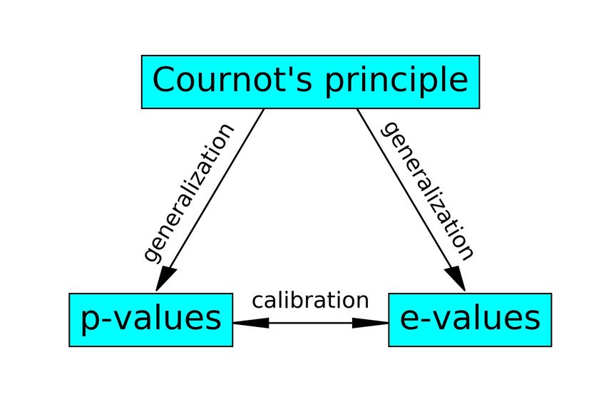
that this is the only bridge.) See Figure 1.
Figure 1: Cournot’s principle and its two generalizations
Cournot’s principle requires an a priori choice of a rejection region E. Its
disadvantage is that it is binary: either the null hypothesis is completely rejected
or we find no evidence whatsoever against it. A p-variable is a nonnegative
random variable p such that, for any α ∈ (0, 1), P (p ≤ α) ≤ α; one way to
define p-variables is via Shafer’s (3). An e-variable is a nonnegative random
variable e such that EP (e) ≤ 1; one way to define e-variables is via Shafer’s
first displayed equation in Section 2. In p-testing, we choose a p-variable p in
advance and reject the null hypothesis P when the observed value of p (the
p-value) is small, and in e-testing, we choose an e-variable e in advance and
reject the null hypothesis P when the observed value of e (the e-value) is large.
In both cases, binary testing becomes graduated: now we have a measure of the
amount of evidence found against the null hypothesis.
We can embed Cournot’s principle into both p-testing,
(
α if y ∈ E
p(y) :=
1 if not,
and e-testing (as Shafer [16, Section 2.1, (1)] explains),
(
1/α if y ∈ E
e(y) :=
0 if not,
where α := P (E).
There are numerous ways to transform p-values to e-values (to calibrate
them) and essentially one way (e 7→ 1/e) to transform e-values to p-values,
5as discussed in detail in [23]. The idea of calibrating p-values originated in
Bayesian statistics ([1, Section 4.2], [19, Section 9], [13]), and there is a wide
range of admissible calibrators. Transforming e-values into p-values is referred
to as e-to-p calibration in [23], where e 7→ 1/e is shown to dominate any e-to-p
calibrator [23, Proposition 2.2].
Moving between the p-domain and e-domain is, however, very inefficient.
Borrowing the idea of “round-trip efficiency” from energy storage, let us start
from the highly statistically significant (≤ 1%) p-value 0.5%, transform it to an
e-value using Shafer’s [16, (6)] calibrator
1
S(0.005) = √ − 1 ≈ 13.14,
0.005
and then transform it back to a p-value using the only admissible e-to-p cali-
brator: 1/13.14 ≈ 0.076. The resulting p-value of 7.6% is not even statistically
significant (> 5%).
A.2 Some comparisons
Both p-values and e-values have important advantages, and I think they should
complement (rather than compete with) each other. Let me list a few advantages
of each that come first to mind. Advantages of p-values:
• P-values can be more robust to our assumptions (perhaps implicit). Sup-
pose, for example, that our null hypothesis is simple. When we have a
clear alternative hypothesis (always assumed simple) in mind, the likeli-
hood ratio has a natural property of optimality as e-variable (Shafer [16,
Section 2.2]), and the p-variable corresponding to the likelihood ratio as
test statistic is also optimal (Neyman–Pearson lemma [11, Section 3.2,
Theorem 1]). For some natural classes of alternative hypotheses, the re-
sulting p-value will not depend on the choice of the alternative hypothesis
in the class (see, e.g., [11, Chapter 3] for numerous examples; a simple
example can be found in [20, Section 4]). This is not true for e-values.
• There are many known efficient ways of computing p-values for testing
nonparametric hypotheses that are already widely used in science.
• In many cases, we know the distribution of p-values under the null hy-
pothesis: it is uniform on the interval [0, 1]. If the null hypothesis is
composite, we can test it by testing the simple hypothesis of uniformity
for the p-values. A recent application of this idea is the use of conformal
martingales for detecting deviations from the IID model [21].
Advantages of e-values (starting from advantages mentioned by Shafer [16, Sec-
tion 1]):
• As Shafer [16] convincingly argues, betting scores are more intuitive than
p-values. Betting intuition has been acclaimed as the right approach to
uncertainty even in popular culture [5].
6• Betting can be opportunistic, in Shafer’s words [16, Sections 1 and 2.2].
Outcomes of experiments performed sequentially by different research
groups can be combined seamlessly into a nonnegative martingale [18]
(see also [8, Section 1]).
• Mathematically, averaging e-values still produces a valid e-value, which
is far from being true for p-values [24]. This is useful in, e.g., multiple
hypothesis testing [23] and statistical testing with data splitting [20].
• E-values appear naturally as a technical tool when applying the duality
theorem in deriving admissible functions for combining p-values [22].
7You can also read