Measuring Global Economic Activity - UC San Diego Department of ...
←
→
Page content transcription
If your browser does not render page correctly, please read the page content below
Measuring Global Economic Activity                          ∗

                                    James D. Hamilton
                           University of California at San Diego
                                   jhamilton@ucsd.edu

                                      August 15, 2018
                                 revised: August 20, 2018

                                        Abstract

   A number of economic studies have used a proxy for world real economic activity derived
from shipping costs. The measure turns out to depend on a normalization that has substantive
consequences of which users of the index have been unaware. This note describes alternative
measures that avoid this and other problems with the commonly used proxy.

   ∗
    I thank the JP Morgan Center for Commodities for financial support as a JPMCC Dis-
tinguished Visiting Fellow.

                                             1
Obtaining a monthly measure of the level of global economic activity faces a number of
challenges; see Kilian (2009) and Kilian and Zhou (2018) for a catalog of some of the concerns.
For this reason, Kilian (2009) proposed using the cost of shipping to construct an alternative
proxy for global economic activity. His measure has since been used in dozens of studies.1
Figure 1 illustrates the basic motivation for how we might use the cost of shipping to infer
something about economic activity. In a typical year, increasing global real economic activity
shifts the demand for shipping to the right, which by itself would lead to an increase in the
price. Increases in shipping capacity and improvements in shipping productivity also shift
the supply curve to the right, leading to lower prices. The trend in real shipping costs has
been downward over time, meaning that in most years the second effect is bigger than the
first. Kilian (2009) suggested that growth in shipping capacity, improvements in shipping
productivity, and growth of potential real GDP could be characterized by deterministic time
trends, and proposed interpreting the residuals from a regression of the real cost of shipping
on a time trend as the cyclical component of global real economic activity.
As a first step in constructing his index of real economic activity, Kilian (2009) developed
a monthly measure xt of the nominal cost of shipping. This was calculated by initializing
x1968:1 = 1 and for each subsequent month through 2007:12 adding an average of the change
in the natural logarithm across a set of different shipping costs to the previous month’s value
xt−1 ,
I
δit ∆ log pit
xt = xt−1 + i=1 I for t = 1968:2, 1968:3, ...,2007:12
i=1 δit
where pit is the cost of shipping a particular bulk dry cargo i and δit = 1 if that cost is known
for t and t − 1. For data since 2008, Kilian and Murphy (2014) updated xt using the Baltic
Dry Index (BDI) of shipping costs:
xt = xt−1 + ∆ log(BDIt ) for t ≥ 2008:1. (1)
Kilian has subsequently continued to update xt using equation (1) and report on his website
a measure of real economic activity described below.
Kilian thought the appropriate way to convert his nominal index xt into a real index would
be to divide xt by the consumer price index (CP It ). He took the log of this ratio, thinking
it was like the log of a relative price:
log(xt /CP It ) = log(xt ) − log(CP It ).
1
See Baumeister and Peersman (2013), Charnavoki and Dolado (2014), Gargano and Timmermann (2014),
Juvenal and Petrella (2014), Kilian and Murphy (2014), Lütkepohl and Netšunajev (2014), Anzuini, Pagano
and Pisani (2015), Antolín-Díaz and Rubio-Ramírez (forthcoming), and Wieland (forthcoming), among many
others.
2He then regressed this difference on a linear time trend:
log(xt ) − log(CP It ) = α + βt + εt . (2)
The residuals εt from this regression are the Kilian index of real economic activity that has
been used by the studies cited in footnote 1 and many others. This index is plotted in the
top panel of Figure 2.
One feature of this construction that appears not to have been understood by the many
users of this index is the following. Equation (1) implies that for t ≥ 2008:1,
xt = x2008:1 + log(BDIt ) − log(BDI2008:1 )
= log(BDIt ) + c0 (3)
for c0 = x2008:1 − log(BDI2008:1 ). No one seems to have noticed the simple identity in (3),
and Kilian has never made public his data for the underlying index xt .2 However, it turns
out to be possible to uncover the underlying series for xt from publicly available data. For
t ≥ 2008:1, the unknown value for xt is related to the observed value of BDIt according
to equation (3) which involves a single unknown constant c0 . We further know that zt =
log(log(BDIt ) + c0 ) − log(CP It ) − α − βt should be exactly equal to the value for εt reported
by Kilian for t ≥ 2008:1 for some values of c0 , α, and β. The values of c0 , α, and β can be
estimated by a nonlinear least squares regression of the reported εt on the value of zt using
data after 2008 and CP I for the vintages used in Kilian and Murphy (2014) or Kilian’s web
page. The resulting estimated values for c0 , α, and β give the fitted regression an R2 of unity
in explaining εt , confirming that we have exactly replicated Kilian’s procedure. With α and
β thus known, the pre-2008 values of xt are then obtained by adding back in the time trend
to εt .3
The uncovered series for xt is plotted in the bottom panel of Figure 2. The value for c0
turns out to be −5.236 when x1968:1 is normalized to be unity. However, if the sequence xt had
been generated with some initial value for x1968:1 other than unity (corresponding to choosing
some month other than 1968:1 to be normalized to unity), the value of c0 would be a different
number. For example, if we started the recursion from a value of x1968:1 that results in a value
for x1973:1 of 1, the value of c0 would be −5.694.
The implications of this can be seen when we substitute (3) into (2):
log[log(BDIt ) + c0 ] − log(CP It ) = α + βt + εt . (4)
2
If Kilian had made his nominal index xt public, someone would have noticed the error to which I call
attention below years ago.
3
Data and code for all calculations and series produced in this paper are available at
http://econweb.ucsd.edu/~jhamilto/REA.zip.
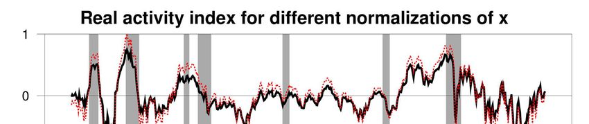
3Taking logs twice is an uncommon procedure for economic data. One consequence of its
application in this context is that the resulting series for real economic activity εt would be
different depending on the value of c0 , that is, different depending on whether we normalize
x1968:1 to be 1, x1973:1 to be 1, or choose some other month to normalize to be 1. Figure 3
shows how different normalizations affect the resulting measure of real economic activity.
After seeing an initial version of this paper, Kilian (2018) acknowledged the problems with
constructing an index based on (2), and now proposes a new measure of real economic activity
based on the residuals of the regression
xt − log(CP It ) = α + βt + εt . (5)
But either equation (4) or equation (5) relies on the strong assumption that there exist values
for α and β that completely capture changes over time in shipping capacity, productivity, and
potential real GDP, so that the resulting series for εt isolates the effects of cyclical movements
in real economic activity. This is a rather strong claim. In practice, the trend is constantly
re-estimated with changing coefficients. When estimated using data through 2009:8 (the
sample period used by Kilian and Murphy, 2014), the intercept of (2) is α̂ = −0.05 and the
slope coefficient β̂ implies an annual decline rate of 2.3%. When estimated using data through
2018:6, the intercept is α̂ = +0.02 and the annual decline rate is 2.8%.
Does the Kilian index correspond to other things we know about global business conditions?
The original Kilian real activity index (obtained from the residuals of (2) with x1968:1 = 1) is
reproduced in the top panel of Figure 4. This series invites us to conclude that there was
a drop in world economic activity in 2016 that was far more severe than that in either the
financial crisis of 2008-2009 or the 1974-75 global recession. The same is also true of the
residuals from (5). That conclusion seems hard to justify on the basis of output data we have
for any major country.
There are some appealing alternatives. OECD Main Economic Indicators published an
estimate of monthly industrial production for the OECD plus 6 other major countries (Brazil,
China, India, Indonesia, the Russian Federation and South Africa). The OECD series ends
in 2011:10, but Baumeister and Hamilton (2018) reproduced the methodology by which the
original index was constructed to extend the series through 2017:12. If we want to isolate a
cyclical component of the series, Hamilton (forthcoming) suggested that the two-year change
in the log offers a simple and robust way to remove the trend in series like this. The resulting
estimate of the cyclical component of industrial production in the OECD plus 6 is plotted in
the second panel of Figure 4. Unlike the Kilian measure, this series implies that the 1974-75
and 2008-2009 recessions were clearly the most significant downturns in global real activity
during this period. The series also suggests that there was a period of strong growth following
the recovery from the 2008-2009 downturn, and characterizes 2015-2016 as sluggish growth
4rather than a separate severe global contraction.
If one were committed to constructing a proxy for global economic activity from the cost
of shipping, a more natural measure would use the log of the relative price rather than the
double-log transformation. Since xt is already in units of a constant plus the log of shipping
costs, the log of the relative price is given simply by πt = xt − log(CP It ). Again the preferred
way to isolate the cyclical component is to take the 2-year difference πt − πt−24 rather than
deviations from a constantly re-estimated time trend. The values of πt − πt−24 are plotted in
the last panel of Figure 4. Like the middle panel, this would again lead us to conclude that
1974-75 and 2008-2009 were the two most significant downturns.
One important benefit of using a price series like the BDI is that it is available at the
daily level,4 allowing us to calculate a version of πt at the daily level. Doing so raises two
modest technical challenges. First, the CP I is only available with a lag, and second, the CP I
only changes at monthly intervals. To solve these issues, I associated the value of the BDI
for the first business day in March with the CP I for January, and interpolated between the
January and February CP I to fill in each subsequent day in March. The two-year difference
of πτ = xτ − log(CP Iτ ) for τ a daily index is plotted in Figure 5, and could in the spirit of
Kilian (2009) be viewed as a daily measure of the cyclical component of global real economic
activity.
I conclude that either the second or third panels of Figure 4 are better measures of the
cyclical component of world economic activity than the index proposed by Kilian. Moreover,
the method used in the third panel can easily be used to construct a daily measure that can
be continuously updated.
4
Daily values for the BDI were obtained from TradingEconomics.com.
5References
Antolín-Díaz, Juan, and Juan F. Rubio-Ramírez (forthcoming). "Narrative Sign Restric-
tions for SVARs," American Economic Review.
Anzuini, Alessio, Patrizio Pagano, and Massimiliano Pisani (2015). "Macroeconomic Ef-
fects of Precautionary Demand for Oil," Journal of Applied Econometrics 30: 968-986.
Baumeister, Christiane, and James D. Hamilton (2018). "Structural Interpretation of
Vector Autoregressions with Incomplete Identification: Revisiting the Role of Oil Supply and
Demand Shocks," Working paper, UCSD.
Baumeister, Christiane, and Gert Peersman (2013). "The Role of Time-Varying Price
Elasticities in Accounting for Volatility Changes in the Crude Oil Market," Journal of Applied
Econometrics 28: 1087-1109.
Charnavoki, Valery, and Juan J. Dolado (2014). "The Effects of Global Shocks on
Small Commodity-Exporting Economies: Lessons from Canada," American Economic Jour-
nal: Macroeconomics 6: 2017-2037.
Gargano, Antonio, and Allan Timmermann (2014). "Forecasting Commodity Price Indexes
Using Macroeconomic and Financial Predictors," International Journal of Forecasting 30: 825-
884.
Hamilton, James D. (forthcoming). "Why You Should Never Use the Hodrick-Prescott
Filter," Review of Economics and Statistics.
Juvenal, Luciana, and Ivan Petrella (2014). "Speculation in the Oil Market," Journal of
Applied Econometrics 30: 621-649.
Kilian, Lutz (2009). "Not All Oil Price Shocks Are Alike: Disentangling Demand and
Supply Shocks in the Crude Oil Market," American Economic Review 99: 1053-1069.
Kilian, Lutz (2018). "Measuring Global Economic Activity: Reply," working paper, Uni-
versity of Michigan.
Kilian, Lutz, and Daniel P. Murphy (2014). "The Role of Inventories and Speculative
Trading in the Global Market for Crude Oil," Journal of Applied Econometrics 29: 454-478.
Kilian, Lutz, and Xiaoqing Zhou (2018). "Modeling Fluctuations in the Global Demand
for Commodities," Journal of International Money and Finance 88: 54-78.
Lütkepohl, Helmut, and Aleksei Netšunajev (2014). "Disentangling Demand and Supply
Shocks in the Crude Oil Market: How to Check Sign Restrictions in Structural VARs," Journal
of Applied Econometrics 29: 479-496.
Wieland, Johannes (forthcoming). "Are Negative Supply Shocks Expansionary at the Zero
Lower Bound?" Journal of Political Economy.
6St St+1
Relative
price P
t
Pt+1
Dt Dt+1
Quantity
Figure 1. World market for shipping services.
7Figure 2. Kilian’s monthly index of real economic activity and underlying nominal index, 1968:1 to
2018:6.
Notes to Figure 2. Top panel: calculated by the author from the residuals from regression (2) when x1968:1
is normalized at 1. Bottom panel: constructed by the author as described in the text. Shaded regions
denote NBER recession dates.
8Figure 3. Residuals from regression (2) for two different normalizations for the level of xt .
9Figure 4. Three different monthly measures of global real economic activity, 1960:1 to 2018:6.
Notes to Figure 4. Top panel: Kilian measure. Middle panel: 2-year change in log of industrial
production for OECD countries plus 6 others. Third panel: 2-year change in difference between xt and the
log of the CPI.
102
1.5
1
0.5
0
-0.5
-1
-1.5
-2
2011 2012 2013 2014 2015 2016 2017 2018
Figure 5. Daily cyclical component of real shipping cost, March 16, 2011 to July 16, 2018.
11You can also read