Common-Envelope Episodes that lead to Double Neutron Star formation
←
→
Page content transcription
If your browser does not render page correctly, please read the page content below
Publications of the Astronomical Society of Australia (PASA)
                                               doi: 10.1017/pas.2020.xxx.

                                               Common–Envelope Episodes that lead to Double
                                               Neutron Star formation
arXiv:2001.09829v3 [astro-ph.SR] 21 Jul 2020

                                               Alejandro Vigna-Gómez1,2,3,4,? , Morgan MacLeod5 , Coenraad J. Neijssel2,3,4 , Floor S.
                                               Broekgaarden5,3,4 , Stephen Justham6,7,8 , George Howitt9,4 , Selma E. de Mink5,8 , Serena
                                               Vinciguerra10,3,4 , Ilya Mandel3,4,2
                                               1 DARK, Niels Bohr Institute, University of Copenhagen, Blegdamsvej 17, 2100, Copenhagen, Denmark
                                               2 Birmingham Institute for Gravitational Wave Astronomy and School of Physics and Astronomy, University of Birmingham,
                                               Birmingham, B15 2TT, United Kingdom
                                               3 Monash Centre for Astrophysics, School of Physics and Astronomy, Monash University, Clayton, Victoria 3800, Australia
                                               4 The ARC Center of Excellence for Gravitational Wave Discovery – OzGrav
                                               5 Harvard-Smithsonian Center for Astrophysics, 60 Garden Street, Cambridge, MA, 02138, USA
                                               6 School of Astronomy & Space Science, University of the Chinese Academy of Sciences, Beijing 100012, China
                                               7 National Astronomical Observatories, Chinese Academy of Sciences, Beijing 100012, China
                                               8 Anton Pannekoek Institute for Astronomy, University of Amsterdam, Postbus 94249, 1090 GE Amsterdam, The Netherlands
                                               9 School of Physics, University of Melbourne, Parkville, Victoria, 3010, Australia
                                               10 Max Planck Institute for Gravitational Physics (Albert Einstein Institute), D-30167 Hannover, Germany
                                               ? Email: avignagomez@nbi.ku.dk

                                               Abstract
                                               Close double neutron stars have been observed as Galactic radio pulsars, while their mergers have been
                                               detected as gamma–ray bursts and gravitational–wave sources. They are believed to have experienced
                                               at least one common–envelope episode during their evolution prior to double neutron star formation. In
                                               the last decades there have been numerous efforts to understand the details of the common-envelope
                                               phase, but its computational modelling remains challenging. We present and discuss the properties of
                                               the donor and the binary at the onset of the Roche-lobe overflow leading to these common–envelope
                                               episodes as predicted by rapid binary population synthesis models. These properties can be used as
                                               initial conditions for detailed simulations of the common–envelope phase. There are three distinctive
                                               populations, classified by the evolutionary stage of the donor at the moment of the onset of the
                                               Roche-lobe overflow: giant donors with fully–convective envelopes, cool donors with partially–convective
                                               envelopes, and hot donors with radiative envelopes. We also estimate that, for standard assumptions,
                                               tides would not circularise a large fraction of these systems by the onset of Roche-lobe overflow. This
                                               makes the study and understanding of eccentric mass-transferring systems relevant for double neutron
                                               star populations.

                                               Keywords: binaries – neutron stars – mass transfer – common envelope – population synthesis

                                               1 INTRODUCTION                                                     one CEE (Ivanova et al., 2013a).
                                                                                                                     While CEEs are frequently invoked as a fundamen-
                                               A dynamically-unstable mass transfer episode initiated             tal part of binary evolution, the detailed physics re-
                                               by a post-main-sequence donor is likely to lead to a               main poorly understood (Paczynski, 1976; Iben & Livio,
                                               common-envelope episode (CEE), in which one star en-               1993; Ivanova et al., 2013b). There have been efforts
                                               gulfs its companion and the binary spiral closer under             in modelling and understanding the phase through hy-
                                               the influence of drag forces (Paczynski, 1976). CEEs are           drodynamic simulations, using Eulerian adaptive mesh
                                               proposed as a solution to the problem of how initially             refinement (Sandquist et al., 1998; Ricker & Taam, 2008;
                                               wide binaries, whose component stars may expand by                 Passy et al., 2012; Ricker & Taam, 2012; MacLeod &
                                               tens to thousands of solar radii during their lifetime,            Ramirez-Ruiz, 2015; Staff et al., 2016; MacLeod et al.,
                                               become close binaries at later stages of evolution (van            2017b; Iaconi et al., 2017, 2018; Chamandy et al., 2018;
                                               den Heuvel, 1976). Most evolutionary pathways leading              De et al., 2019; Li et al., 2020; López-Cámara et al.,
                                               to close compact binaries are expected to involve at least         2019; Shiber et al., 2019), moving meshes (Ohlmann
                                                                                                              1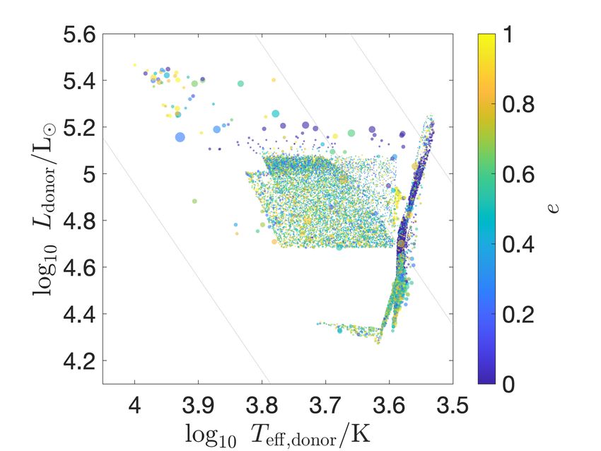
2                                                                                                   Vigna-Gómez et al.

et al., 2016, 2017; Prust & Chang, 2019), smoothed par-        which may be signatures of common-envelope ejections
ticle (Rasio & Livio, 1996; Lombardi et al., 2006; Nan-        (Ivanova et al., 2013b; MacLeod et al., 2017a; Blagorod-
dez et al., 2015; Nandez & Ivanova, 2016; Passy et al.,        nova et al., 2017; Pastorello et al., 2019; Howitt et al.,
2012; Ivanova & Nandez, 2016; Reichardt et al., 2019),         2020), and Be X-ray binaries (Vinciguerra et al., 2020).
particle-in-cell (Livio & Soker, 1988) and general rela-          This paper is structured in the following way. Section
tivistic (Cruz-Osorio & Rezzolla, 2020) methods. Other         2 describes the initial distributions and relevant physical
approaches pursue detailed stellar modeling (Dewi &            parameterisations used in rapid population synthesis.
Tauris, 2000; Kruckow et al., 2016; Clayton et al., 2017;      Section 3 presents the results of our study, particularly
Fragos et al., 2019; Klencki et al., 2020) or binary popu-     Hertzsprung-Russell (HR) diagrams displaying different
lation synthesis (e.g. Tauris & Bailes, 1996; Nelemans         properties of the systems, as well as their distributions.
et al., 2000; Dewi et al., 2006; Andrews et al., 2015;         Section 4 discusses the results and some of the caveats.
Kruckow et al., 2018; Vigna-Gómez et al., 2018). There        Finally, section 5 summarises and presents the conclu-
is currently no consensus on a thorough understanding          sions of this work.
of CEEs on all the relevant spatial and time scales.
   Recent rapid population synthesis studies of double
                                                               2 POPULATION SYNTHESIS MODEL
neutron star (DNS) populations have been partially mo-
tivated by the development of gravitational-wave astron-       We characterise CEEs with the rapid population syn-
omy. Software tools such as StarTrack (Dominik et al.,         thesis element of the COMPAS suite2 (Stevenson et al.,
2012; Belczynski et al., 2018; Chruslinska et al., 2017,       2017; Barrett et al., 2018; Vigna-Gómez et al., 2018;
2018), MOBSE (Giacobbo & Mapelli, 2018, 2019a,b,               Neijssel et al., 2019). Rapid population synthesis re-
2020), C o m B i n E (Kruckow et al., 2018) and COM-           lies on simplified methods and parameterisations in or-
PAS (Vigna-Gómez et al., 2018; Chattopadhyay et al.,          der to simulate a single binary from the zero-age main-
2020) have been used to explore synthetic DNS popula-          sequence (ZAMS) until stellar merger, binary disruption
tions in detail. Most of those studies focus on predicting     or double compact object (DCO) formation. This ap-
or matching the observed DNS merger rate, either by            proach relies on sub-second evolution of a single binary
investigating different parameterisations of the physics       in order to generate a large population within hours
or varying the parameters within the models. In particu-       using a single processor.
lar, all of the aforementioned population synthesis codes         In COMPAS, an initial binary is defined as a
follow a similar simplified treatment of the common            gravitationally-bound system completely specified by
envelope (CE) phase.                                           its metallicity, component masses, separation and eccen-
   In this paper, we present a detailed analysis of the        tricity at the ZAMS. We assume that our binaries have
CEEs that most merging DNSs are believed to experi-            solar metallicity Z = Z = 0.0142 (Asplund et al., 2009).
ence at some point during their formation (Bhattacharya        The mass of the primary (m1 ), i.e. the more massive star
& van den Heuvel, 1991; Belczynski et al., 2002; Ivanova       in the binary at birth, is drawn from the initial mass
et al., 2003; Dewi & Pols, 2003; Dewi et al., 2005; Tauris     function dN/dm1 ∝ m−2.3 1    (Kroupa, 2001) sampled be-
& van den Heuvel, 2006; Andrews et al., 2015; Tauris           tween 5 ≤ m1 /M ≤ 100. The mass of the secondary
et al., 2017; Belczynski et al., 2018; Kruckow et al., 2018;   (m2 ) is obtained by drawning from a flat distribution
Vigna-Gómez et al., 2018). Dominik et al. (2012) pre-         in mass ratio (qZAMS = m2 /m1 ) in the form dN/dq ∝ 1
viously used rapid population synthesis to study the           with 0.1 < qZAMS ≤ 1 (Sana et al., 2012). The initial
relationship between CEEs and DNS merger rates. In             separation is drawn from a flat-in-the-log distribution in
this study, we focus our attention on the properties at        the form dN/da ∝ a−1 with 0.01 < aZAMS /AU < 1000
the onset of the Roche-lobe overflow (RLOF) episode            (Öpik, 1924). We assume that all our binaries have zero
leading to the CEE. We consider both long-period non-          eccentricity at formation (the validity of this assumption
merging DNSs as well as short-period merging DNSs. We          is discussed in Section 4.4.3).
propose these distributions of binary properties as initial
conditions for detailed studies of CEEs. We provide the
                                                               2.1 Adaptive Importance Sampling
results of this study in the form of a publicly available
catalogue1 .                                                   COMPAS originally relied on Monte Carlo sampling
   We examine the properties of binaries unaffected by         from the birth distributions described above. However,
external dynamical interactions that experience CEEs           this becomes computationally expensive when studying
on their way to forming DNS systems. We briefly dis-           rare events.
cuss CEEs leading to DNS formation in the context of              In order to efficiently sample the parameter space
generating some of the brightest luminous red novae,           leading to DNS formation, we adopt STROOPWAFEL as
                                                               implemented in COMPAS (Broekgaarden et al., 2019).
   1 The   database and resources can be found           on
https://zenodo.org/record/3593843 (Vigna-Gómez, 2019)           2 https://compas.science/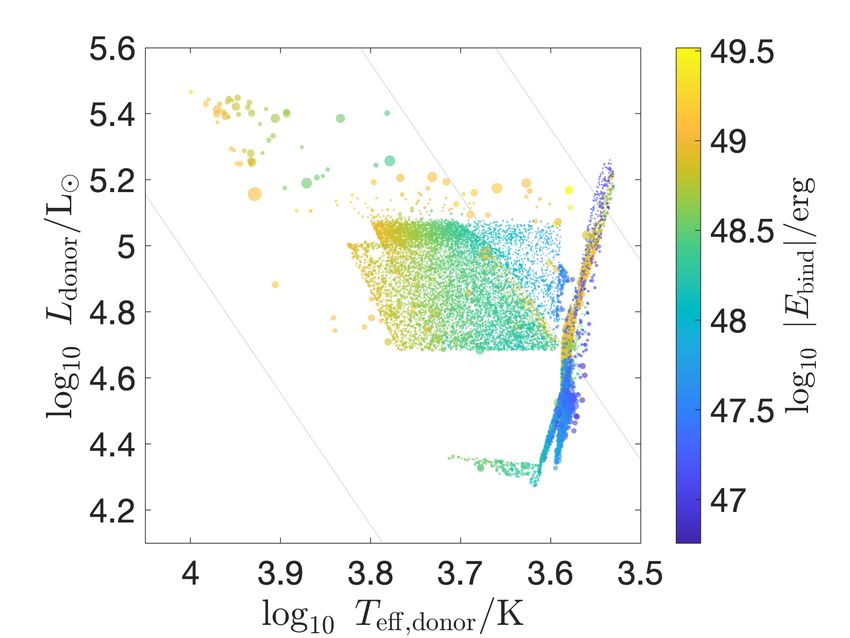
CEEs that lead to DNS formation                                                                                      3

STROOPWAFEL is an adaptive importance sampling (AIS)           leads to a CEE. Inspired by Ge et al. (2015), for
algorithm designed to improve the efficiency of sam-           main-sequence (MS) donors, we assume ζdonor =
pling of unusual astrophysical events. The use of AIS          2.0; for Hertzsprung gap (HG) donors, we assume
increases the fraction of DNSs per number of binaries          ζdonor = 6.5. For post-helium-ignition phases in
simulated by ∼ 2 orders of magnitude with respect to           which the donor still has a hydrogen envelope, we
regular Monte Carlo sampling. After sampling from a            follow Soberman et al. (1997). All mass transfer
distribution designed to increase DNS yield, the binaries      episodes from stripped post-helium-ignition stars,
are re-weighted by the ratio of the desired probability        i.e. case BB mass transfer (Delgado & Thomas,
distribution of initial conditions to the actual sampling      1981; Dewi et al., 2002; Dewi & Pols, 2003) onto a
probability distribution.                                      neutron star (NS) are assumed to be dynamically
   We use bootstrapping to estimate the sampling uncer-        stable. For more details and discussion, see Tauris
tainty. We randomly re-sample each model population            et al. (2015) and Vigna-Gómez et al. (2018).
with replacement in order to generate a bootstrapped        3. We deviate from Stevenson et al. (2017) and Vigna-
distribution. We perform this process N = 100 times to         Gómez et al. (2018) by allowing MS accretors to
get a 10% accuracy of the bootstrapped standard devia-         survive a CEE. Previously, any MS accretor was
tion. We calculate and report the standard deviation of        mistakenly assumed to imminently lead to a stellar
the bootstrapped distributions as 1σ error bars.               merger. We now treat MS accretors just like any
                                                               other stellar type. This does not have any effect
                                                               on the COMPAS DNS population, as there are no
2.2 Underlying Physics
                                                               dynamically unstable mass transfer phases with MS
We mostly follow the physical model as presented in            accretors leading to DNS formation (see discussion
Vigna-Gómez et al. (2018). However we highlight key           on formation history in Section 3.1).
aspects of the model that are particularly relevant for     4. We follow de Kool (1990) in the parameterization
this work, along with a few non-trivial changes to the         of the binding energy (Ebind ) of the donor star’s
code. See also Appendix A for a summary and additional         envelope (mdonor,env ) given as:
details on the setup.
 1. We approximate the Roche-lobe radius following                                   −Gmdonor mdonor,env
                                                                           Ebind =                       ,         (4)
    the fitting formula provided by Eggleton (1983) in                                   λRdonor
    the form:
                            2/3
      RRL          0.49qRL                                       where G is the gravitational constant and λ is a
          =     2/3          1/3
                                  , 0 < qRL < ∞, (1)             numerical factor that parameterises the binding
       ap   0.6qRL + ln(1 + qRL )
                                                                 energy.
    where RRL is the effective Roche-lobe radius of the     5.   For the value of the λ parameter, we follow the
    donor, ap = a(1 − e) is the periastron, a and e are          fitting formulae from detailed stellar models as cal-
    the semi-major axis and eccentricity respectively,           culated by Xu & Li (2010a,b). This λ, originally
    qRL is the mass ratio; qRL = mdonor /mcomp , with            referred to as λb , includes internal energy and is
    mdonor and mcomp being the mass of the donor and             implemented in the same way as λNanjing in Star-
    companion star, respectively. RLOF will occur once           Track (Dominik et al., 2012). Additionally, we fixed
    Rdonor ≥ RRL , where Rdonor is the radius of the             a bug which underestimated the binding energy of
    donor.                                                       the envelope. We discuss the effect this has on the
 2. We use the properties of the system at the onset             DNS population in Section 3.2.
    of RLOF in order to determine whether the mass          6.   We use the αλ-formalism (Webbink, 1984; de Kool,
    transfer episode leads to a CEE. Dynamical stability         1990) to determine the post-CEE orbit, with α = 1
    is determined by comparing the response of the               in all of our CEEs.
    radius of the donor to (adiabatic) mass loss to the     7.   We use the Fryer et al. (2012) delayed supernova
    response of the Roche-lobe radius to mass transfer.          remnant mass prescription, which was the preferred
    This is done using the mass-radius exponent                  model from Vigna-Gómez et al. (2018). This pre-
                                                                 scription allows for a continuous (gravitational) rem-
                               d log Ri                          nant mass distribution between NSs and black-holes,
                     ζi =                ,           (2)
                            d log mdonor                         with a transition point at 2.5 M .
    where the subscript “i” represents either the mass-     8.   The remnant mass of NSs with large baryonic mass
    radius exponent for the donor (ζdonor ) or for the           previously only accounted for neutrino mass loss
    Roche lobe (ζRL ). We assume that                            instead of an actual equation of state. This has now
                                                                 been corrected. This only affects NSs with remnant
                        ζdonor < ζRL                 (3)         masses larger than ≈ 2.15 M .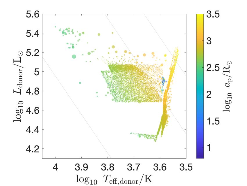
4                                                                                                    Vigna-Gómez et al.

2.3 Tidal Timescales                                          2.3.1 The equilibrium tide for stars with convective
                                                                    envelopes
Mass transfer episodes occur in close binaries that ex-
                                                              Under the equilibrium tide, the synchronisation and
perienced tidal interactions. The details of these tidal
                                                              circularisation evolution equations for tides acting on
interactions are sensitive to the properties of the binary
                                                              a star of mass mtide from a companion star with mass
and the structure of the envelope of the tidally distorted
                                                              mcomp are
stars, either radiative or convective.
   The equilibrium tide refers to viscous dissipation in                            2       6
                                                                  dΩspin         k    q Rtide       Ωorb
a star that is only weakly perturbed away from the                        =3           2
                                                                    dt         τtide rg     a     (1 − e2 )6
shape that it would have in equilibrium (Zahn, 1977).                                                          (5)
Meanwhile, the dynamical tide (Zahn, 1975) refers to                                2         2 3/2    2 Ωspin
                                                                            × f2 (e ) − (1 − e ) f5 (e )
the excitation of multiple internal modes of a star in                                                    Ωorb
a time-varying gravitational potential; when these os-        and
cillatory modes are damped, orbital energy is lost to                                            8
thermal energy (Eggleton et al., 1998; Moe & Kratter,           de            k               Rtide         e
                                                                   = − 27          q(1 + q)
2018). Tidal evolution tends to align and synchronise           dt          τtide               a      (1 − e2 )13/2
                                                                                                                     (6)
the component spins with the direction of the orbital
                                                                                   11

                                                                             2              2 3/2     2 Ωspin
angular momentum vector and circularise the binary                   × f3 (e ) − (1 − e ) f4 (e )               ,
                                                                                   18                    Ωorb
(Counselman, 1973; Zahn, 2008).
   There are numerous uncertainties in tidal evolution.       where fn (e2 ) are polynomial expressions given by Hut
For example, the role of eccentricity is an active field      (1981). The structure of the tidally deformed star is
of research. Heartbeat stars are eccentric binaries with      parameterised by k, which is the apsidal motion constant
close periastron passage which experience tidal excita-       (Lecar et al., 1976) and the intrinsic tidal timescale
tion of different oscillatory modes (see Shporer et al.       (τtide ), usually associated with viscous dissipation (Zahn,
2016 and references therein). Eccentric systems may           1977). We follow Hurley et al. (2002) in the calculation of
also experience resonance locking, which occurs when a        the (k/τtide ) factor, which depends on the evolutionary
particular tidal harmonic resonates with a stellar oscil-     stage and structure of the star. The mass ratio is defined
lation mode; this enhances the efficiency of tidal dissipa-   as q =pmcomp /mtide = 1/qRL and the gyration radius as
                                                              rg = Itide /(mtide Rtide 2 ), where I
tion (Witte & Savonije, 1999a,b). The high-eccentricity                                              tide and Rtide are the
regime, previously studied in the parabolic (and chaotic)     moment of inertia and the radius of the tidally deformed
limit (Mardling, 1995a,b), has recently being revisited       star, respectively. The mean orbital velocity and the
in the context of both dynamical (Vick & Lai, 2018)           donor spin angular velocity are denoted by Ωorb and
and equilibrium tides (Vick & Lai, 2020). There are           Ωspin , respectively.
uncertainties in the low-eccentricity regime: for example,       Given that a > Rtide , for a non-synchronous eccentric
there is a range of parameterisations for the equilibrium     binary we expect synchronisation to be faster than circu-
tide, such as the weak friction approximation, turbulent      larisation. If we assume that the system is synchronous
viscosity and fast tides (Zahn, 2008).                        (Ωorb = Ωspin ), we simplify Equation (6) and estimate
   Here, we make several simplifying approximations for       the circularisation timescale as
the synchronisation and circularisation timescales, τsync                      e
                                                                τcirc = −
and τcirc respectively, in order to parameterise the tidal                  de/dt
evolution of the system.                                                                            8
                                                                                  k               Rtide         1
   We assume that the equilibrium tide operates on all                 = 27             q(1 + q)                         (7)
                                                                                τtide              a       (1 − e2 )13/2
stars with a convective envelope, regardless of the binary                                                  −1
eccentricity. We use the equilibrium tide description in                                 11
                                                                          × f3 (e2 ) − (1 − e2 )3/2 f4 (e2 )        .
the weak friction model as described by Hut (1981) and                                   18
implemented by Hurley et al. (2002), although this may
not be accurate for high-eccentricity systems (but see        2.3.2 The dynamical tide for stars with radiative
Vick & Lai 2020). Since the equilibrium tide is generally           envelopes
a more efficient energy transport/dissipation mechanism       Following the derivation by Zahn (1977) we can write
than the dynamical tide for stars with convective en-         the synchronisation and circularisation timescales for
velopes, we ignore the contribution of the latter. Our        the dynamical tide as
equilibrium tide model is summarised in Section 2.3.1.                               3      1/2 2
                                                                               −5/3   Rtide       rg
   We apply the dynamical tide only to stars with a                  τsync = 52                      (1 + q)−5/6
radiative envelope. In Section 2.3.2 we present our imple-                           Gmtide       q2
                                                                                           17/2                (8)
mentation of the dynamical tide following Zahn (1977),                           −1    D
as used in Hurley et al. (2002).                                             × E2
                                                                                      Rtide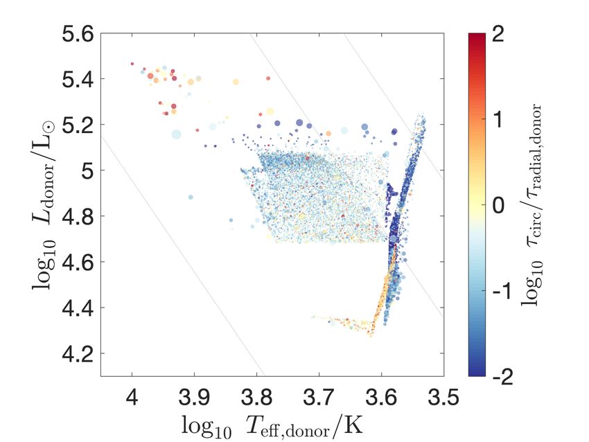
CEEs that lead to DNS formation                                                                                           5

and                                                            culation of k and τtide follows Hurley et al. (2000) and
                     1/2                           21/2      is uncertain for massive stars. For the radial expansion
                           (1 + q)−11/6 −1
             3
          2    Rtide                           D               timescale, the fitting formulae we use are not accurate
 τcirc =                               E2                 ,
         21 Gmtide               q            Rtide            in representing the evolution of the star on thermal or
                                                        (9)    dynamical timescales. These formulae also miss detailed
where E2 = 1.592 × 10⁻⁹ (M/M )2.84 is a second-order           information about the evolution of, e.g., the size of the
tidal coefficient as fitted by Hurley et al. (2002) from       convective envelope. Additionally, they are not accurate
the values given by Zahn (1975), under the assumption          in representing the effect of mass loss and mass gain.
(violated for some of the systems we consider) that close
binaries are nearly circular. For the dynamical tide, we
set the tidal separation (D) to be the semilatus rectum        3 RESULTS
D = a(1 − e2 ). This corresponds to p   the conservation
of orbital angular momentum Jorb ∝ a(1 − e2 ). This            We present the results of the synthetic population of
assumption may lead us to underestimate the circular-          binaries which become DNSs. We focus our attention
isation timescale for stars with radiative envelopes in        on the properties of the systems at the onset of the
highly eccentric orbits.                                       CEE. If a donor star experiences RLOF, leading to a
   The dynamical tide is much less efficient than the          dynamically unstable mass transfer episode, the system
equilibrium tide for virtually all binaries; therefore, we     is classified as experiencing a CEE. In that case we report
ignore the contribution of dynamical tides for convective-     the properties of the system at the moment of RLOF. We
envelope stars, even though they are active along with         do not resolve the details of the CEE, such as the possible
equilibrium tides.                                             delayed onset of the dynamical inspiral phase. Given
   Given the uncertainties in tidal circularisation effi-      that we are interested in DNS progenitors, all of these
ciency, we do not include tides in dynamical binary            CEEs will, by selection, experience a successful ejection
evolution. Instead, we evolve binaries without the im-         of the envelope, i.e. no stellar mergers are reported in this
pact of tides, then estimate whether tides would have          study. All the data presented in this work are available
been able to circularise the binary prior to the onset of      at https://zenodo.org/record/3593843 (Vigna-Gómez,
RLOF leading to a CEE as described below.                      2019).

2.3.3 Radial expansion timescale                                  Our synthetic data set contains about 1,000,000 bina-
                                                               ries evolved using COMPAS. Out of all the simulated
The strong dependence of the tidal timescales on Rtide /a
                                                               binaries, targeted at DNS-forming systems (see Section
means that tides only become efficient when the star ex-
                                                               2.1), there are 15,201 CEEs leading to DNS formation.
pands to within a factor of a few of the binary separation.
                                                               These provide a far more accurate sampling of the ≈365
Therefore, the rate of expansion of the star, which de-
                                                               systems that would be expected for 86,000,000 M of
pends on the stage of stellar evolution, plays a key role in
                                                               star-forming mass sampled from the initial conditions.
determining the efficiency of circularisation: the binary
                                                               For simplicity, we assume 100% binarity a priori. Never-
can circularise only if the circularisation timescale of an
                                                               theless, given our assumed separation distribution that is
eccentric binary is shorter than the star’s radial expan-
                                                               capped at 1000 AU, 10% of our systems never experience
sion timescale. We define this radial expansion timescale
                                                               any mass transfer episode, resulting in two effectively
as the radial e-folding time τradial ≡ dt/d log R. This is
                                                               single stars. While DNSs are believed to form in dif-
computed by evaluating the local derivatives within the
                                                               ferent environments, several studies have shown that
fitting formulae of Hurley et al. (2000) to the detailed
                                                               metallicity does not play a large role in DNS properties,
stellar models from Pols et al. (1998).
                                                               unlike binary black hole or neutron star/black hole for-
2.3.4 Uncertainties in timescales                              mation (Dominik et al., 2012; Vigna-Gómez et al., 2018;
                                                               Giacobbo & Mapelli, 2018; Neijssel et al., 2019).
The timescales defined here, rather than fully accurate
descriptions of tidal evolution, are used as order of mag-        The results section is structured as follows. Section
nitude estimates to analyse the overall properties of          3.1 discusses the two dominant formation channels in
the population. Tidal timescales have significant un-          our model, i.e. the evolutionary history of the binary
certainties, including in the treatment of the dominant        from ZAMS to DNS formation. Section 3.2 we present
dissipation mechanism (e.g. weak friction approximation,       a comparison with the results from Vigna-Gómez et al.
turbulent convection, fast tides) and their parameteri-        (2018). In Section 3.3 we describe the way main results
sation (Zahn, 2008) and implementation (Hurley et al.,         are presented. In Section 3.4 we report the properties of
2002). Siess et al. (2013) noted the problem with the          the donor. In section 3.5 we report the properties of the
E2 fit being commonly misused, both via interpolation          binary, in particular the orbital properties. Finally, in
and extrapolation of stars above 20 M (see also the            Section 3.6 we present and report the tidal circularisation
alternative approach of Kushnir et al. 2017). The cal-         timescales.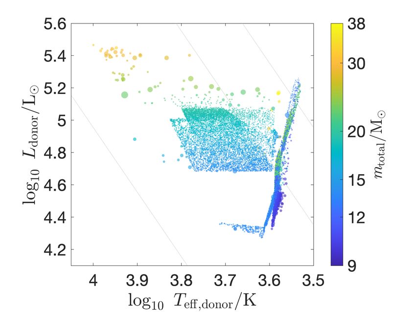
6                                                                                                     Vigna-Gómez et al.

Table 1 Properties of the donor star and the binary at the onset of RLOF leading to a CEE. In this Table, we list the
symbols and units for each parameter, as well as the figure where the parameter is presented.

                               Property                         Symbol               Units   Figure
                              Luminosity                         Ldonor               L         2
                        Effective temperature                  Teff,donor              K        2
                             Stellar phase                          -                  -        2
                                 Mass                           mdonor                M       3, 10
                            Envelope mass                      menv,donor             M         -
                              Core mass                       mcore,donor             M         -
                          Core mass fraction          fdonor ≡ mcore,donor /mdonor     -        3
                      Radial expansion timescale              τradial,donor          Myr      6, 8
                            Binding energy                      |Ebind |              erg      3,9
                             Eccentricity                           e                  -        4
                           Semi-major axis                          a                 R       9,10
                              Periastron                     ap = a(1 − e)            R       4,10
                           Companion mass                        mcomp                M        10
                              Total mass               mtotal = mdonor + mcomp        M         5
                              Mass ratio                  q = mcomp /mdonor            -       5,9
                       Circularisation timescale                  τcirc              Myr      6, 8

3.1 Formation Channels of Double Neutron                        phase. Rapid population synthesis modelling of CEEs
    Star systems                                                sometimes parameterise these donors in two possible
                                                                outcomes: optimistic and pessimistic (Dominik et al.,
Two common evolutionary pathways leading to the
                                                                2012). The optimistic approach assumes the donor
formation of DNS from isolated binary evolution are
                                                                has a clear core/envelope separation and that, as a
identified in the literature (Bhattacharya & van den
                                                                result, the two stellar cores can potentially remove the
Heuvel, 1991; Tauris & van den Heuvel, 2006; Tauris
                                                                common envelope, allowing the binary to survive the
et al., 2017). Following Vigna-Gómez et al. (2018), we
                                                                CEE. Throughout this paper, we assume the optimistic
refer to these formation channels as Channel I and
                                                                approach unless stated otherwise. The pessimistic
Channel II.
                                                                approach assumes that dynamically unstable mass
                                                                transfer from a HG donor leads imminently to a merger.
  Channel I is illustrated in the top panel of Figure 1
                                                                The pessimistic approach results in 4% of potential
and proceeds in the following way:
                                                                DNS candidates merging before DCO formation.
    1. A post-MS primary engages in stable mass transfer
       onto a MS secondary.                                       Channel II is illustrated in the bottom panel of Figure
    2. The primary, now stripped, continues its evolution       1 and proceeds in the following way:
       as a naked helium star until it explodes in a super-
                                                                 1. A dynamically unstable mass transfer episode leads
       nova, leaving a NS remnant in a bound orbit with
                                                                    to a CEE when the primary and the secondary are
       a MS companion.
                                                                    both post-MS star. During this CEE, both stars
    3. The secondary evolves off the MS, expanding and
                                                                    have a clear core-envelope separation, and they en-
       engaging in a CEE with the NS accretor.
                                                                    gage in what is referred to in the literature as a
    4. After successfully ejecting the envelope, and hard-
                                                                    double-core CEE (Brown, 1995; Dewi et al., 2006;
       ening the orbit, the secondary becomes a naked
                                                                    Justham et al., 2011). For these binaries, evolu-
       helium star.
                                                                    tionary timescales are quite similar, with a mini-
    5. The stripped post-helium-burning secondary en-
                                                                    mum and mean mass ratio of ≈ 0.93 and ≈ 0.97
       gages in highly non-conservative stable (case BB)
                                                                    respectively, consistent with high-mass and low-
       mass transfer onto the NS companion.
                                                                    mass solar metallicity values reported in Dewi et al.
    6. After being stripped of its helium envelope, the
                                                                    (2006). During this double-core CEE, both stars are
       ultra-stripped secondary (Tauris et al., 2013, 2015)
                                                                    stripped and become naked-helium-stars.
       continues its evolution until it explodes as an ultra-
                                                                 2. The stripped post-helium-burning primary engages
       stripped SN (USSN), forming a DNS.
                                                                    in stable (case BB) mass transfer onto a stripped
   In Channel I the CEE may occur while the donor                   helium-burning secondary.
is crossing the HG, i.e. between the end of the MS               3. The primary, now a naked metal star, explodes in
and the start of the core helium burning (CHeB)                     a supernova (SN) and becomes a NS.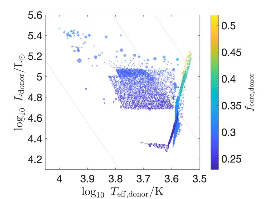
CEEs that lead to DNS formation 7
4. There is a final highly non-conservative stable (case temperature (Teff,donor ) and stellar type of the donor.
BB) mass transfer episode from the stripped post- In the case of a double-core CEE, the donor is defined
helium-burning secondary onto the NS. as the more evolved star from the binary, which is the
5. The secondary then explodes as an USSN, forming primary in Channel II.
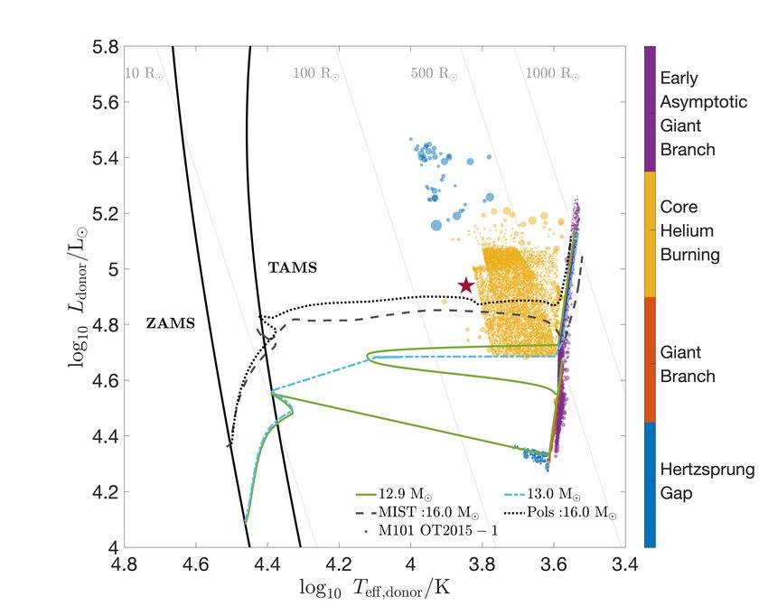
a DNS. In Figure 2, there is a visually striking feature: the
almost complete absence of systems which forms a white
The two dominant channels, Channel I and Channel II, polygon around log10 (Ldonor /L ) = 4.5. This feature
comprise 69% and 14% of all DNSs in our simulations is a consequence of the fitting formulae used for single
(Z = 0.0142), respectively. The remaining formation stellar evolution (c.f. Figures 14 and 15 of Hurley et al.
channels are mostly variations of the dominant chan- 2000). This white region is bounded by the evolution of a
nels. These variations either alter the sequence of events 12.9 M and a 13.0 M star at Z=0.0142. The MS evo-
or avoid certain mass transfer phases. Some formation lution of both stars is quite similar. After the end of the
scenarios rely on fortuitous SN kicks. Some other ex- MS, there is a bifurcation point arising from the lower
otic scenarios, which allow for the formation of DNS in mass system experiencing a blue loop and the higher
which neither neutron star is recycled by accretion (e.g. mass system avoiding it. This bifurcation is enhanced by
Belczyński & Kalogera, 2001), comprise less than 2% of the sharp change in the Teff − L slope from the interpola-
the DNS population. tion adopted by Hurley et al. (2000) during the HG phase.
This change in slope around log10 (Ldonor /L ) = 4.5 and
3.2 Comparison with Vigna-Gómez et al. log10 (Teff,donor /K) = 4.4 is model-dependent, but we do
(2018) expect to have some differences in the evolution of stars
around that mass. This bifurcation corresponds to the
This work generally uses similar assumptions and physics transition around the First Giant Branch, which sep-
parameterisations as the preferred model of Vigna- arates intermediate-mass and high-mass stars. Stellar
Gómez et al. (2018), including the Fryer et al. (2012) tracks from Choi et al. (2016) also display a bifurcation
delayed supernova engine. Although the qualitative re- point, but models and interpolation are smoother than
sults are similar, there are some quantitative changes those in Hurley et al. (2000).
due to updated model choices and corrections to the A rare example of how a system could end up in the
COMPAS population synthesis code as described in Sec- forbidden region is the following. If a star experiences a
tion 2.2 and Appendix A. For example, the percentage of blue loop, it contracts and then re-expands before contin-
systems forming though Channel I remains ≈ 70%, but uing to evolve along the giant branch. If the companion
now only ≈ 14% of systems experience Channel II, in- experiences a supernova with a suitable kick while the
stead of ≈ 21% in Vigna-Gómez et al. (2018). The main star is in this phase, and the orbit is modified appropri-
change concerns the DNS rates which in this work are a ately in the process, the system may experience RLOF.
factor of a few lower than those in the preferred model of A fortuitous kick making the orbit smaller, more eccen-
Vigna-Gómez et al. (2018). Here, we estimate the forma- tric, or both, would be an unusual but not implausible
tion rate of all (merging) DNS to be 85(60) Gpc−3 yr−1 . outcome of a SN.
Vigna-Gómez et al. (2018) reports the formation rate
of all (merging) DNS to be 369(281) Gpc−3 yr−1 for
the preferred model. We discuss rates in more detail in 3.4 Properties of the Donor
Section 4.4.6. We report the luminosity, effective temperature, stel-
lar phase, mass and core mass fraction of the donor
3.3 Common-Envelope Episodes leading to (fdonor ≡ mcore,donor /mdonor ), as presented in Table 1.
Double Neutron Star Formation in the The luminosity and effective temperature limits are
Hertzsprung-Russell Diagram log10 [Ldonor,min /L , Ldonor,max /L ] = [4.3, 5.5] and
log10 [Teff,donor,min /K, Teff,donor,max /K] = [3.5, 4.0], re-
For all properties, we present a colour coded HR dia- spectively. In Figure 2 we highlight the stellar phase,
gram, normalised distribution and CDF. In Figure 2, which is colour-coded. While the evolution in the HR
we present our synthetic population of DNS progeni- diagram is itself an indicator of the evolutionary phase of
tors at the onset of RLOF leading to a CEE. They are the star, our stellar models follow closely the stellar-type
coloured according to the stellar type of the donor at nomenclature as defined in Hurley et al. (2000). Donors
RLOF, which is specified using the nomenclature from which engage in a CEE leading to DNS formation can
Hurley et al. (2000)3 . Additionally, Figure 2 shows the be in the HG (4%), GB (7%), CHeB (59%) or EAGB
normalised distributions of luminosity (Ldonor ), effective (30%) phase.
3 We use the early asymptotic giant branch (EAGB) nomencla- In the case of Channel I, donors are HG or CHeB stars;
ture even for stars with masses m ' 10 M which do not become they span most of the parameter space from terminal-
AGB stars. age MS until the end of core-helium burning, with a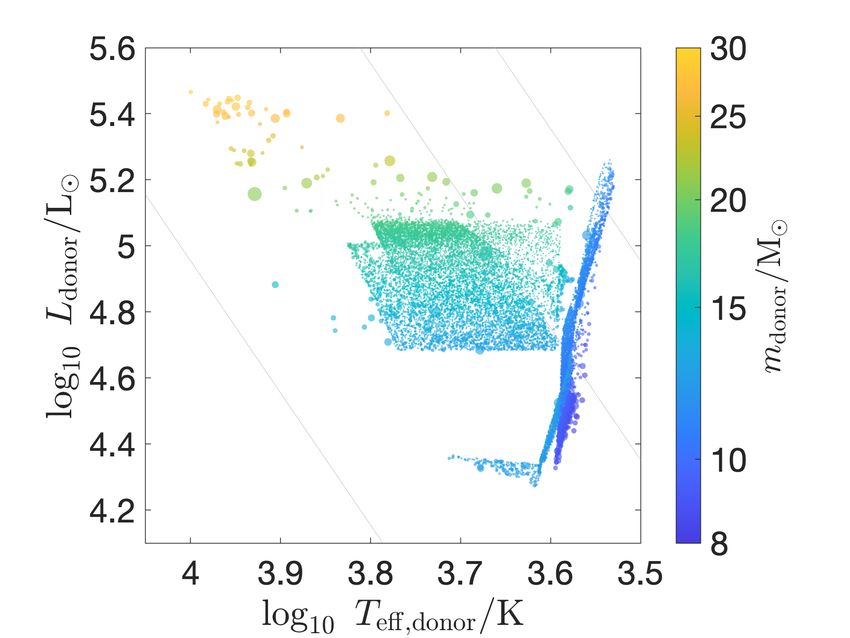
8                                                                                                               Vigna-Gómez et al.

                                                        CHANNELI

            ZAMS                        RL
                                         OF                         Pos
                                                                      t-
                                                                       RLOF                         SN

                   NS                      CEE                  Pos
                                                                  t-
                                                                   CEE           Cas
                                                                                   eBBRL
                                                                                       OF                USSN             DNS

                                                        CHANNELI
                                                               I

             ZAMS                            CEE                       Pos
                                                                         t-
                                                                          CEE                    Cas
                                                                                                   eBBRL
                                                                                                       OF

                   SN                         NS                  Cas
                                                                    eBBRL
                                                                        OF                   USSN                   DNS

Figure 1. Schematic representation of DNS formation channels as described in Section 3.1. Top: Channel I is the dominant formation
channel for DNS systems, as well as the most common formation channel in the literature (see, e.g., Tauris et al. 2017 and references
therein). Bottom: Formation Channel II distinguished by an early double-core common-envelope phase. Acronyms as defined in text.
Credit: T. Rebagliato.
CEEs that lead to DNS formation                                                                                                           9

Figure 2. Main properties of the donor star at the onset of RLOF leading to the CEE in DNS-forming binaries. Top: HR diagram
coloured by stellar phase: HG (blue), GB (orange), CHeB (yellow) and EAGB (purple). The sizes of the markers represent their sampling
weight. We show the progenitor of the luminous red nova M101 OT2015-1 (Blagorodnova et al., 2017) with a star symbol. The solid
black lines indicate ZAMS and TAMS loci for a grid of SSE models (Hurley et al., 2000) at Z ≈ 0.0142. We show the evolution of a
single non-rotating 16 M star, from ZAMS to the end of the giant phase: the dotted dark-grey line shows a MIST stellar track from
Choi et al. (2016) and the dashed grey line shows the stellar track from Pols et al. (1998, 2009). The dash-dotted light-blue and solid
green lines show how fitting formulae from Hurley et al. (2000) lead to a bifurcation after the MS for stars with masses between 12.9
and 13.0 M . This bifurcation is related to which stars are assumed to begin core-helium-burning while crossing of the HG or only after
it: see the presence (lack) of the blue loop in the 12.9 (13.0) M track. Grey lines indicate stellar radii of R = {10, 100, 500, 1000} R .
Bottom: Normalised distributions in blue (left vertical axis) and CDFs in orange (right vertical axis) of luminosity (left panel), effective
temperature (middle panel) and stellar type (right panel). Black error bars indicate 1σ sampling uncertainty in the histograms. Grey
lines show 100 bootstrapped distributions that indicate the sampling uncertainty in the CDFs. The CDFs show a subset of 365 randomly
sampled values, which is the same number of DNS in our population, for each bootstrapped distribution.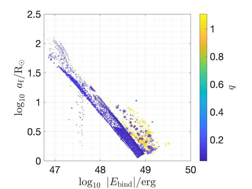
10                                                                                                   Vigna-Gómez et al.

temperature range of ∼ 0.5 dex. In the case of Channel II,    are [ap,min , ap,max ] ≈ [7, 3100] R . (Very rarely, even
donors are GB or EAGB giant-like stars. The parameter         smaller periapses are possible when fortuitous super-
space in the HR diagram for these giant-like donors is        nova kicks send the newly formed NS plunging into the
significantly smaller, spanning an effective temperature      envelope of an evolved companion on a very eccentric
range of only ∼ 0.1 dex.                                      orbit; however it is not clear whether such events lead
   The limits in the mass of the donor are [mdonor,min ,      to a CEE or to a more exotic outcome, such as the
mdonor,max ] = [8, 29] M . The core mass fraction,            formation of a Thorne & Żytkow 1977 object). The to-
shown in Figure 3, has limits of [fcore,donor,min ,           tal mass distribution, shown in Figure 5, has limits of
fcore,donor,max ] = [0.2, 0.5]. The core mass fraction can    [mtotal,min , mtotal,max ] = [9, 37] M .
serve as a proxy for the evolutionary phase.                     We compute the mass ratio at the onset of the RLOF
   We report the binding energy of the envelope (see          leading to the CEE. The mass ratio, shown in Figure
Figure 3) as defined in Equation 4. In the case of            5, has limits of [qmin , qmax ] = [0.05, 1.11]. The broad
a double-core CEE, the binding energy of the com-             distribution in fact consists of two distinct peaks, one
mon envelope is assumed to be Ebind = Ebind,donor +           close to q = 0 and the other close to q = 1, with a large
Ebind,comp . The binding energy falls in the range            gap between 0.18 ≤ q ≤ 0.98 (see Figure 5). The extreme
log10 (−[Ebind,min , Ebind,max ]/erg) = [49.5, 46.8]. The     mass ratio systems correspond to CEEs from Channel
systems with the most tightly bound envelopes, and            I, where the companion is a NS. The q ≈ 1 systems
therefore the lowest (most negative) binding energies,        correspond to CEEs from Channel II, where there is a
are those experiencing a CEE shortly after TAMS or as         double-core CEE with a non-compact companion star.
double-core CEEs. For double-core systems, the enve-          The systems with q > 1 are double-core CE systems
lope of the less evolved companion is more bound than         with qZAMS ≈ 1 which, at high metallicity, may reverse
the one of the more evolved donor star.                       their mass ratio via mass loss through winds before the
                                                              primary star expands and undergoes RLOF.
3.5 Properties of the Binary
                                                              3.6 Tidal Timescales in
We also report the properties of each binary by
                                                                  Pre-Common-Envelope Systems
colour coding the property of interest in the HR di-
agram. We report the eccentricity, semi-major axis,           Given the uncertainties in the treatment of tides, and
total mass (mtotal = mcomp + mdonor ), mass ratio             our interest in comparing the impact of different tidal
(q = mcomp /mdonor ) and the ratio of the circularisa-        prescriptions as discussed below (see Section 4.4.2), we
tion timescale (τcirc ) to the radial expansion timescale     do not include tidal synchronisation or circularisation
(τradial ), as presented in Table 1. All quantities are re-   in binary evolution modelling for this study. Instead,
ported at the onset of the RLOF unless stated otherwise.      we consider whether tides would be able to efficiently
   The eccentricity, semi-major axis and masses of the        circularise the binary before the onset of RLOF leading
system determine the orbital energy and angular momen-        to a CEE. As discussed in Section 2.3.3, we use the ratio
tum of a binary (in the two point-mass approximation).        of the circularisation timescale to the radial expansion
The eccentricity and semi-major axis distributions shown      timescale as a proxy for the efficiency of tidal circulari-
in Figure 4 do not account for tidal circularisation. The     sation of an expanding star about to come into contact
eccentricities span the entire allowed parameter range        with its companion. If τcirc /τradial,donor > 1, we label the
0 ≤ e < 1. The eccentricity distribution has a sharp          binary as still eccentric at RLOF. Given that the circu-
feature around e ≈ 0. Systems with e ≈ 0 are typically        larisation timescale is longer than the synchronisation
those from Channel II, where the double-core CEE hap-         timescale (see Section 2.3), we focus on the former and
pens as the first mass-transfer interaction, without any      assume that if the binary is able to circularise, it will
preceding supernova to make the binary eccentric given        already be synchronous.
our assumption of initially circular binaries (further dis-      Figure 6 shows the ratio τcirc /τradial,donor under our
cussion of this choice is in Section 4.4.3). Meanwhile, the   default assumption in which both HG and CHeB stars
most eccentric binaries have the smallest periapses and       have fully convective envelopes for the purpose of tidal
interact the earliest during the evolution of the donor,      circularisation calculations and experience the equilib-
explaining the trend of greater eccentricities for smaller    rium tide. This assumption results in 82% of the systems
donor sizes in Figure 4.                                      being circular at the onset of RLOF.
   The semi-major axis distribution, shown in Figure             The analysis of circularisation timescales is mostly
4, has limits of [amin , amax ] = [330, 7000000] R . The      relevant for systems formed through Channel I (see
very few extremely wide systems correspond to very            Section 4.4.2). There are two reasons for this. The first
eccentric binaries, almost unbound during the super-          one is that they are expected to acquire a non-zero
nova explosion (e.g. e ≈ 0.9999 for the widest binary).       eccentricity after the first supernova. The second one
While those limits are broad, the limits in periastron        is that they are more likely to have a radiative or only
CEEs that lead to DNS formation 11 Figure 3. Pre-CEE donor properties of all DNS-forming systems: mass (top), core mass fraction (middle), and envelope binding energy (bottom). The core mass fraction is defined as fcore,donor ≡ mcore,donor /mdonor . In the case of a double-core CEE, the binding energy is the sum of the individual envelope binding energies. Yellow systems with binding energies larger than log10 |Ebind /erg| ≈ 48.5 during the red supergiant phase are double-core CEE systems. For more details, see Section 3.4. See the caption of Figure 2 for further explanations.
12                                                                                                                  Vigna-Gómez et al.

Figure 4. Pre-CEE orbital properties of all DNS-forming systems. The binary properties presented are eccentricity (top) and semi-major
axis (bottom). The orbital properties do not account for tidal circularisation. For more details, see Section 3.5. See the caption of Figure
2 for further explanations.
CEEs that lead to DNS formation                                                                                              13

Figure 5. Pre-CEE mass of all DNS-forming systems. The binary properties presented are total mass (top) and mass ratio (bottom).
For more details, see Section 3.5. See the caption of Figure 2 for further explanations.
14                                                                                                  Vigna-Gómez et al.

partially convective envelope, making circularisation less    the dynamical stability of mass transfer. In particular,
efficient. On the other hand, systems formed through          hot donors lacking a deep convective envelope may be
Channel II have a fully-convective envelope, which allows     stable to mass transfer and avoid a CEE. At the same
for efficient tidal circularisation and synchronisation. We   time, some of the less evolved hot donors may not survive
apply the low-eccentricity approximation described in         a CEE even if they do experience dynamical instability
Section 2.3.1 to computing the tidal timescales of these      (pessimistic variation).
systems, even though they are circular by construction          Klencki et al. (2020) use detailed stellar evolution
before the first SN (we discuss this assumption in Section    models to argue that only red supergiant donors with
4.4.3).                                                       deep convective envelopes are able to engage in and
                                                              survive a CEE. For their assumptions, this would reduce
4 DISCUSSION                                                  the estimated rate of DNS formation. However, and
                                                              similar to this study, they focus on RLOF structures
In this section we discuss the properties of CEEs expe-       and not the structures at the moment of the instability.
rienced by isolated stellar binaries evolving into DNSs
and present some of the caveats in our COMPAS rapid              Here, we focus only on the impact of the assumed
population synthesis models.                                  structure of the donor on the efficiency of tidal circulari-
                                                              sation and do not account for possible consequences for
                                                              mass transfer stability. We compare three alternative
4.1 Common-Envelope Episode                                   models in Figure 8.
    Sub-populations in Evolving Double
                                                                 Our default tidal circularisation model assumes that
    Neutron Stars
                                                              all evolved donors, including both HG and CHeB stars,
4.1.1 Formation channels                                      have fully convective envelopes, and therefore experience
There are two main formation channels leading to DNS          efficient equilibrium tides. Our default assumption esti-
formation. Channel I involves high mass ratio single-core     mates that 18% of systems will be eccentric at the onset
CEE between a NS primary and a post-MS secondary.             of the RLOF leading to the CEE. This is the lowest frac-
Channel I has been studied thoroughly in the literature,      tion of eccentric systems among all variations because
e.g. Bhattacharya & van den Heuvel (1991); Tauris &           tides are particularly efficient for stars with convective
van den Heuvel (2006); Tauris et al. (2017) and refer-        envelopes.
ences therein. Channel II involves a double-core common          In reality, CHeB stars are expected to begin the CHeB
envelope between two post-MS stars. A similar channel         phase with a radiative envelope and develop a deep con-
has been proposed by Brown (1995) and Dewi et al.             vective envelope by the end of it. The single stellar fits
(2006), among others. Channel II requires similar masses      from Hurley et al. (2000) do not contain explicit infor-
at ZAMS driven by the need of similar evolutionary            mation about the moment when this transition occurs.
timescales so that both stars are post-MS giants at the       Hurley et al. (2002) assume that all CHeB stars have a
time of their first interaction. For low (high) mass stars,   radiative envelope and that the dynamical tide is domi-
the difference in ZAMS mass can be up to 3 (7)%, in           nant in their tidal evolution. Adopting this assumption
agreement with Dewi et al. (2006). Our Channel II has an      leads to 68% of binaries remaining eccentric at the onset
additional case BB mass transfer episode from a helium-       of the RLOF leading to the CEE.
shell-burning primary onto a helium-MS secondary.
                                                                 Alternatively, Belczynski et al. (2008) assume that
4.1.2 Sub-populations and tidal circularisation               hot stars with log10 (Teff /K) > 3.73 have a radiative
We separate CEE donors into three distinct sub-               envelope, while cool stars with log10 (Teff /K) ≤ 3.73
populations depending on their evolutionary phase at          have a convective envelope. Adopting this assumption
the onset of RLOF: giants, cool and hot (see Table 2          leads to 40% of binaries remaining eccentric at the onset
and Figure 7).                                                of the RLOF leading to the CEE.
   The first one, giants, correspond to giant donors             According to our estimates, a significant fraction of
with fully-convective envelopes. The other two sub-           systems will be eccentric at RLOF. These estimates were
populations correspond to HG or CHeB donors, most of          made within the framework of the fitting formulae for
them evolving via the single-core Channel I. We distin-       single stellar evolution from Hurley et al. (2000). More
guish between cool donors with a partially convective         detailed fitting formulae, which include the evolutionary
envelope and hot donors with a radiative envelope. We         stage of stars as well as the mass and radial coordi-
follow Belczynski et al. (2008) in using the temperature      nates of their convective envelopes, would allow for a
log10 (Teff,donor /K) = 3.73 as the boundary between the      self-consistent determination of whether a star has a
cool and hot sub-populations.                                 radiative, a partially convective or a fully convective
   The presence and depth of a convective envelope im-        envelope for both dynamical stability and tidal circular-
pacts the response of the star to mass loss and, hence,       isation calculations.
CEEs that lead to DNS formation 15
Figure 6. Ratio of tidal circularisation timescale to the star’s radial expansion timescale for all DNS-forming systems. We present
the default scenario where all evolved stars, including HG and CHeB stars, are assumed to have formed a fully convective envelope. If
log10 (τcirc /τradial ) ≤ 0, we assume that binaries circularise before the onset of the CEE. Binaries indicated with blue (red) dots are
predicted to have circular (eccentric) orbits. We cap −2 ≤ log10 (τcirc /τradial ) ≤ 2 to improve the plot appearance. The grey shaded
region in the histogram highlights the systems which circularise by the onset of RLOF. For more details, see Section 3.6. See the caption
of Figure 2 for further explanations.
Table 2 Distinct DNS sub-populations as described in Section 4.1 and presented in Figure 7.
Sub-population Threshold Dominant Channel Donor Envelope Colour Fraction
Giants - II (double core) GB, EAGB fully convective blue 0.37
Cool log10 (Teff /K) < 3.73 I (single core) HG, CHeB partially convective orange 0.38
Hot log10 (Teff /K) ≥ 3.73 I (single core) HG, CHeB radiative/convective yellow 0.25
Figure 7. DNS-forming binaries clustered by the donor type at the onset of the CEE. Sub-populations: (a) giant donors with fully-
convective envelopes in blue, (b) HG or CHeB donors with partially-convective envelopes in red, and (c) HG or CHeB donors which
have not yet formed a deep convective envelope in yellow. For more details, see Section 3.4. See the caption of Figure 2 for further
explanations.16 Vigna-Gómez et al.
4.2 Common-Envelope Episodes as
candidates for luminous red novae
transients
Recently, the luminous red nova transient M101 OT2015-
1 was reported by Blagorodnova et al. (2017). This event
is similar to other luminous red novae associated with
CEEs (Ivanova et al., 2013b). Following the discovery
of M101 OT2015-1, archival photometric data from ear-
lier epochs were found. Blagorodnova et al. (2017) used
these to derive the characteristics of the progenitor. The
inferred properties of the progenitor of M101 OT2015-
1 are a luminosity of Ldonor ≈ 87, 000 L , an effec-
tive temperature of Teff,donor ≈ 7, 000 K and a mass of
mdonor = 18 ± 1 M (see Figure 2 for location in the
HR diagram).
Blagorodnova et al. (2017) found that the immediate
pre-outburst progenitor of M101 OT2015-1 was consis-
Figure 8. CDF of the ratio of the circularisation timescale to tent with an F-type yellow supergiant crossing the HG.
the donor radial expansion timescale computed at RLOF onset If we take the inferred values for this star as the values at
leading to CEE for all DNS-forming systems. Here we present the onset of RLOF, then this star is consistent with pre-
three scenarios. The solid blue line is our default assumption: all
donors have a deep convective envelope (same as in left panel of
CEE stars in our predicted distribution of DNS-forming
Figure 6). The red dashed line follows Hurley et al. (2002) with systems. However, we emphasise that the appearance of
the assumption that CHeB tidal evolution is dominated by the the donor star can change significantly between the onset
dynamical tide, i.e. that CHeB stars have a radiative envelope. of RLOF, i.e., the point at which the models shown in
The yellow dotted line follows Belczynski et al. (2008) in assuming
that stars with log Teff ≤ 3.73 K have a fully convective envelope, Figure 2 are plotted, and dynamical instability.
for both HG and CHeB donors; and a fully radiative envelope Howitt et al. (2020) explored population synthesis
otherwise, as in Figure 7. For more details, see Section 3.6. models of luminous red novae. Here we use the same
pipeline adopted for that study to explore the connection
to DNS populations. Doing so, fewer than 0.02% of all
luminous red novae lead to DNSs. These are amongst
the most energetic luminous red novae and would be
over-represented in the magnitude-limited observable
population. Future DNSs constitute nearly 10% of the
subpopulation of luminous red novae with predicted
plateau luminosities greater than 107 L .
4.3 Eccentric Roche-lobe Overflow leading to
a Common-Envelope Episode
We predict that the sub-population of giant donors with
fully-convective envelopes and cool donors with partially-
convective envelopes are likely to be circular at the onset
of the CEE (see Figures 6 and 8). On the other hand, we
find that the sub-population of hot donors often does not
circularise by the onset of the CEE. This sub-population
with hot donors are binaries with high eccentricities at
Figure 9. All DNS-forming binaries from our Fiducial model are the onset of the RLOF (see Figure 4).
shown here. We present the post-CEE separation af as a function of This result raises questions about the initial conditions
the absolute value of the envelope binding energy |Ebind |. For the
double-core scenario, the binding energy is Ebind = Ebind,donor + of a CEE, which is often assumed to begin in a circular or-
Ebind,comp . The size of the marker indicates the sampling weight bit, both in population synthesis studies and in detailed
and its colour shows the mass ratio q. This Figure can be compared simulations. Population synthesis codes such as SEBA
to Figures 1 and 2 from Iaconi & De Marco (2019). That study
(Portegies Zwart & Verbunt, 1996; Portegies Zwart &
presents simulations of CE binaries and observations of post-CE
binaries. Most systems presented here do not feature in Iaconi & Yungelson, 1998; Toonen et al., 2012), STARTRACK (Bel-
De Marco (2019). czynski et al., 2002, 2008), BSE (Hurley et al., 2002), the
Brussels code (De Donder & Vanbeveren, 2004), COM-CEEs that lead to DNS formation 17
Figure 10. Binary separations at CEEs leading to DNSs at the onset of RLOF (left) and after the CEE (right). We show the donor
(mdonor ) and companion (mcomp ) mass in both plots, with a solid grey line indicating mdonor = mcomp . The colour bars, with different
scales, show the pre-CEE periastron (left) and final semi-major axis (right).
PAS (Stevenson et al., 2017; Vigna-Gómez et al., 2018), for low-eccentricity binaries, precisely those which may
ComBinE (Kruckow et al., 2018) and customised soft- efficiently circularise through mass transfer.
ware based on them all assume that RLOF commences Hamers & Dosopoulou (2019) noted that evolution
in circular binaries. Detailed simulations, such as those towards circularisation from Dosopoulou & Kalogera
of Passy et al. (2012), MacLeod et al. (2018) and others, (2016b) could lead to (nonphysical) negative eccentricity
often make the assumption of an initially circular orbit solutions. They proposed a revised analytic model for
(but see Staff et al. 2016, discussed in more detail in mass transfer in eccentric binaries. This study takes
Section 4.3.2). into account the separation and eccentricity evolution of
an initially eccentric system at RLOF. However, their
4.3.1 Theory of mass transfer in eccentric binaries model is only valid in the regime of fully-conservative
Mass transfer in eccentric binaries has been explored mass transfer, and is therefore more restricted than the
with both semi-analytical and analytical methods general formalism Dosopoulou & Kalogera (2016b). Mass
(Matese & Whitmire, 1983, 1984; Sepinsky et al., 2007, transfer episodes in binaries which will become DNSs are
2009, 2010; Dosopoulou & Kalogera, 2016a,b). typically non-conservative. Mass transfer from a post-
The analysis of Sepinsky et al. (2007) et al. assumes MS donor onto a MS companion, such as the first mass
fully conservative mass transfer. While they consider transfer episode from Channel I, is generally only partly
mass transfer from a stellar donor onto a neutron star, conservative (Schneider et al., 2015). Mass transfer onto
this assumption and the typical 10−9 M yr−1 mass a NS companion is highly non-conservative, almost in
transfer rate they consider is relevant for low-mass X- the fully non-conservative limit (Tauris et al., 2015).
ray binaries, not DNS progenitors as discussed here. A full understanding of the evolution of eccentric sys-
tems in RLOF is yet to be achieved. A detailed treatment
Dosopoulou & Kalogera (2016b) study orbital evolu-
of non-conservative mass transfer in an eccentric binary
tion considering both conservative and non-conservative
could yield different criteria for dynamical stability and,
mass transfer. The latter scenario is particularly rele-
ultimately, for determining if a system engages in a CEE.
vant for DNS formation. We assume a mass transfer rate
of 10−5 M yr−1 , a 1.44 M NS and mass loss from
4.3.2 Modelling of mass transfer in eccentric
the vicinity of the NS (isotropic re-emission) as param-
binaries
eters in their Equation (44). Highly eccentric systems
(e > 0.9) have circularisation timescales of more than 1 Numerical methods and simulations have also been used
Myr due to mass transfer, under their assumption that to study mass transfer in eccentric binaries (Regös et al.,
all mass transfer happens at periapsis. This timescale is 2005; Church et al., 2009; Lajoie & Sills, 2011; van der
reduced to around a thousand years for mass transfer in Helm et al., 2016; Staff et al., 2016; Bobrick et al., 2017).
e < 0.1 binaries, although this can be very sensitive to Staff et al. (2016) carried out hydrodynamic simula-
assumptions about the specific angular momentum lost tions of a ≈ 3 M giant star with a less massive MS
at the level of an order of magnitude. The assumption of companion in an eccentric orbit. They conclude that
instantaneous mass transfer at periapsis is questionable eccentric systems transfer mass only during the perias-You can also read