Connectivity and population structure of albacore tuna across southeast Atlantic and southwest indian oceans inferred from multidisciplinary ...
←
→
Page content transcription
If your browser does not render page correctly, please read the page content below
www.nature.com/scientificreports

            OPEN            Connectivity and population
                            structure of albacore tuna
                            across southeast Atlantic
                            and southwest Indian Oceans
                            inferred from multidisciplinary
                            methodology
                            Natacha Nikolic1,2,3,12*, Iratxe Montes4, Maxime Lalire5, Alexis Puech1, Nathalie Bodin6,11,13,
                            Sophie Arnaud‑Haond7, Sven Kerwath8,9, Emmanuel Corse2,14, Philippe Gaspar 5,10,
                            Stéphanie Hollanda11, Jérôme Bourjea1, Wendy West8,15 & Sylvain Bonhommeau 1,15

                            Albacore tuna (Thunnus alalunga) is an important target of tuna fisheries in the Atlantic and
                            Indian Oceans. The commercial catch of albacore is the highest globally among all temperate tuna
                            species, contributing around 6% in weight to global tuna catches over the last decade. The accurate
                            assessment and management of this heavily exploited resource requires a robust understanding
                            of the species’ biology and of the pattern of connectivity among oceanic regions, yet Indian Ocean
                            albacore population dynamics remain poorly understood and its level of connectivity with the Atlantic
                            Ocean population is uncertain. We analysed morphometrics and genetics of albacore (n = 1,874) in the
                            southwest Indian (SWIO) and southeast Atlantic (SEAO) Oceans to investigate the connectivity and
                            population structure. Furthermore, we examined the species’ dispersal potential by modelling particle
                            drift through major oceanographic features. Males appear larger than females, except in South African
                            waters, yet the length–weight relationship only showed significant male–female difference in one
                            region (east of Madagascar and Reunion waters). The present study produced a genetic differentiation
                            between the southeast Atlantic and southwest Indian Oceans, supporting their demographic
                            independence. The particle drift models suggested dispersal potential of early life stages from SWIO to
                            SEAO and adult or sub-adult migration from SEAO to SWIO.

                            1
                             Institut Français de Recherche pour l’Exploitation de la Mer, Délégation de La Réunion, Rue Jean Bertho, BP 60,
                            97 822 Le Port Cedex, La Réunion, France. 2ARBRE, Agence de Recherche pour la Biodiversité la Réunion, 34
                            avenue de la Grande Ourse, 97434 Saint‑Gilles, La Réunion, France. 3IRD, UMR MARine Biodiversity Exploitation
                            and Conservation (MARBEC), Saint‑Clotilde, La Réunion, France. 4Department of Genetics, Physical Anthropology
                            and Animal Physiology, University of the Basque Country (UPV/EHU), Barrio Sarriena s/n, 48940 Leioa,
                            Spain. 5CLS, Sustainable Management of Marine Resources, 11 rue Hermès, 31520 Ramonville Saint‑Agne,
                            France. 6IRD, UMR MARBEC, Fishing Port, Victoria, Seychelles. 7IFREMER, Station de Sète, Avenue Jean Monnet,
                            CS 30171, 34203 Sète Cedex, France. 8Department of Environmental Affairs, Private Bag X2, Vlaeberg 8018,
                            South Africa. 9Department of Biological Sciences, University of Cape Town, Rondebosch, Cape Town 7701, South
                            Africa. 10Mercator Ocean, 10 rue Hermès, 31520 Ramonville Saint‑Agne, France. 11Seychelles Fishing Authority
                            (SFA), Fishing Port, Victoria, Seychelles. 12Present address: UMR INRAE-UPPA 1224 Ecobiop, Aquapole, 173
                            RB918 Route de Saint‑Jean‑de‑Luz, 64310 Saint‑Pée‑sur‑Nivelle, France. 13Sustainable Ocean Seychelles (SOS),
                            BeauBelle, Mahe, Seychelles. 14Centre Universitaire de Formation et de Recherche de Mayotte, MARBEC, 8 rue
                            de l’Université BP53, 97660 Dembeni, Mayotte. 15These authors contributed equally: Wendy West and Sylvain
                            Bonhommeau. *email: natacha.nikolic@inrae.fr

Scientific Reports |   (2020) 10:15657               | https://doi.org/10.1038/s41598-020-72369-w                                         1

                                                                                                                                     Vol.:(0123456789)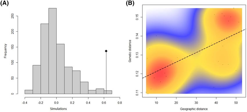
www.nature.com/scientificreports/
Albacore tuna (Thunnus alalunga, Scombridae) is an important, commercially harvested pelagic species with
high migratory capacity, distributed throughout most tropical and temperate oceans, except in the polar r egions1.
The commercial albacore catch is the highest globally among all temperate tuna species, contributing around
6% in weight to global tuna catches over the last decade2,3 and 5% in 20174. Although currently not subject to
overfishing in the South Atlantic and Indian O ceans5,6, there is significant uncertainty about stock assessments
due to the lack of key biological information7,8.
The Indian and the South Atlantic Oceans remain the two least known areas regarding albacore population
structure and connectivity. Life history, biology and population structure information are critical input for stock
assessments and the representation of these parameters has to resemble the actual population structure of the
resource9. In this context ‘population’ is used in the biological and ecological sense (individuals of a species that
live simultaneously in a geographical area and have the ability to reproduce). Regional Fisheries Management
Organizations (RFMOs) currently manage albacore based on six hypothetical populations or stocks (Mediterra-
nean, North Atlantic, South Atlantic, Indian, North Pacific, and South Pacific). The definition of these populations
or stocks have been supported by some genetic studies10–15 but the definition remains controversial, particularly
within an ocean (e.g. between albacore populations of northern and southern hemispheres). Additionally, differ-
ences in delimitation among various methods (i.e. serological, parasitological, proteomic, tagging, morphometric,
genetic) is evident (see Table 1 and 2 in Nikolic and B ourjea16).
Tag-recapture experiments suggest low rates of migration between hemispheres13. The albacore remains
underrepresented in ongoing programs such as the Atlantic Ocean Tuna Tagging Program AOTTP, as these
target mostly tropical species such as bigeye, skipjack and yellowfin tuna. Consequently, migratory exchange
between the South Atlantic and Indian Oceans remains unresolved.
The establishment of an accurate population boundary requires a multidisciplinary approach to which popu-
lation genetics can provide an important contribution17,18. In fact, genetic markers are widely used to investigate
connectivity between populations and to define stocks and the degree of mixture between stocks in a fishery19–21.
Based on catch statistics, M orita22 suggested active inter-oceanic migration of adult albacore between Atlantic and
Indian Oceans off South Africa, which could be promoted by the strong Agulhas Current, as also suggested for the
congeneric bigeye tuna (Thunus obesus)23. Albacore from southwest Africa are usually genetically clustered with
the Atlantic p opulation15,22. Also, in a previous genetic s tudy24 based on samples of albacore from the seas off the
Cape of Good Hope (South Africa), southeast Atlantic and southwest Atlantic observed no heterogeneity. Yet, to
our knowledge, no samples from the southwest Indian and southeast Atlantic Oceans were analyzed to test for
the existence of inter-oceanic migration. The scarce information on the population structure of albacore in the
South Atlantic and Indian Oceans thus warrants further analyses of the population structure and connectivity
of this species in these areas, in order to test Morita’s hypothesis of a significant exchange.
Genetics studies on albacore began with assessing the population structure of this species in the Pacific and
Atlantic Oceans9–12,15,24–28; and more recently, in the Indian Ocean using multi-locus analyses based on nuclear
and mitochondrial genetic markers. These multi-locus analyses include microsatellite markers, which have been
increasingly used during the last decade in fisheries management29. Although recent studies on albacore have
used Single Nucleotide Polymorphism (SNPs, e.g.. 616 and 75 S NPs30,31), the limited number of SNPs used for
this species has not provided high-density genetic map coverage and genome information .
In addition to genetic markers, fish populations can also be discriminated based on variations of morpho-
metric traits32, such as length–weight relationships, which can be the result of either genetic variation and/or
phenotypic responses to variations in local environmental factors33–35. Few length–weight relationship estimates
are available for albacore in the Indian Ocean36.
Dispersal (and thus connectivity) is greatly dependent upon ocean fronts and c urrents37. Since the population
structure of marine pelagic fishes is influenced by physical features of the marine environment, biophysical mod-
elling can be used to predict passive dispersal38. Lagrangian transport models can help to predict the potential
early stage dispersal pattern and extent of connectivity from spawning area to settlement s ites39,40, including over
large scales41, and to assess oceanographic model limitations42. Here, we used Lagrangian simulation of particles
solely drifting with surface currents (i.e. with no active locomotion) to test if connectivity through passive drift
can explain, at least partly, early life stage dispersal of albacore tuna and the genetic structure of the population.
The objective of our study was to investigate the connectivity and population structure of albacore tuna
between the southeast Atlantic (SEAO) and southwest Indian Oceans (SWIO), with multiple methods. We col-
lected genetic and morphometric data from albacore in 2013 and 2014 in four geographic regions to determine
genetic or morphometric differences. We combined these information with the Lagrangian simulation to test if
connectivity through passive drift can explain, at least partly, early life stage dispersal of albacore tuna and the
genetic structure of the population.
Materials and methods
Sampling. Albacore samples were collected from four different geographic regions from June 2013 to August
2014 over two seasons (periods); in the southwest Indian Ocean between the east of Madagascar and Reunion
(region A), and Seychelles to the coast of Somalia (region B), in South African waters (region C), and in the
southeast Atlantic Ocean (region D) (Fig. 1). To account for the variability of environmental conditions and life
history traits, sampling was performed over two seasons (Austral summer: November-February, i.e. potential
reproduction season of tunas; and austral winter: April–August, i.e. potential feeding period or post-reproduc-
tion period8,43) except in geographic region B, and over two years (2013 and 2014) except in geographic region
D (see Appendix 1). They are called sampling locations (A1, A2, B1, B2, C1, C2, D1, and D2) (Fig. 1). Fish from
the waters of geographic region A were sampled on a research trip on board a commercial longliner and from
artisanal fishermen using vertical longlines in the second season. Albacore from the geographic region B were
Scientific Reports | (2020) 10:15657 | https://doi.org/10.1038/s41598-020-72369-w 2
Vol:.(1234567890)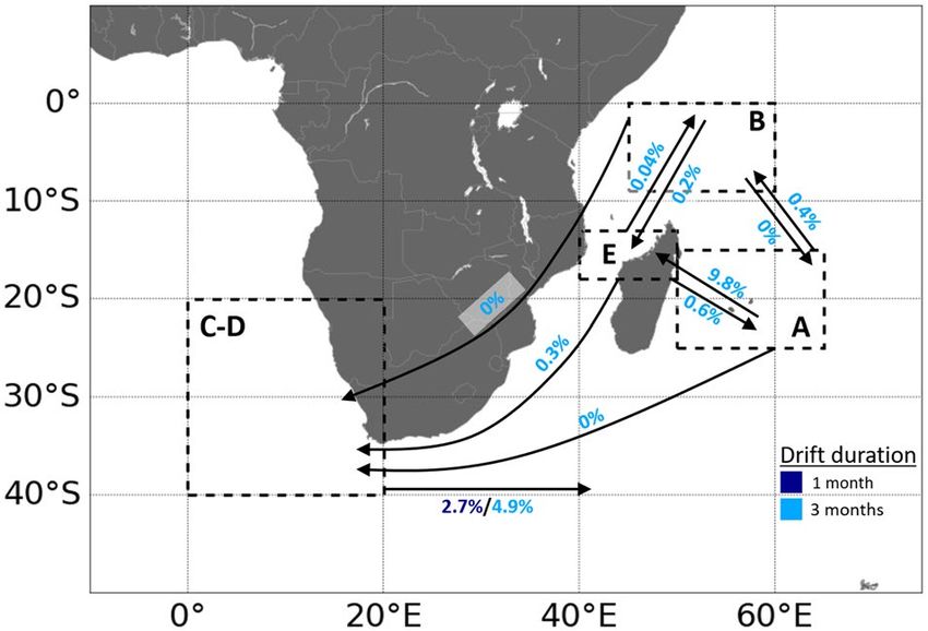
www.nature.com/scientificreports/
Figure 1. Sampling locations of albacore sampled for genetic analysis (total of 1,874 individuals). Circles are
proportional to the number of individuals collected in both periods. Austral summer (1) and Austral winter
(2). (A) East Madagascar (around Reunion Island (A1) n = 236; around Reunion Island and east of Madagascar
(A2) n = 230). (B) North Madagascar ((B1) n = 233; (B2) n = 233). (C) South Africa ((C1) n = 323; (C2) n = 276).
(D) Southeast Atlantic Ocean ((D1) n = 157; (D2) n = 191). Southwest Indian Ocean (SWIO) also mentioned
by (A) and (B) sampling locations. Southeast Atlantic Ocean (SEAO) also mentioned by (C) and (D) sampling
locations. Benguela Current (BC), Agulhas Current (AC), Agulhas Return Current (AR), Somali Current (SC),
Southern Gyre (SG), South Equatorial Counter Current (SECC), and Southeast Madagascar Current (SEMC).
caught by purse-seiners and sampled during processing. Finally, in geographic regions C and D, the samples
were obtained from the catch landed by the commercial pole-and-line fishing boats and at sea by observers. No
ethical approval was required as all fish sampled were dead by sampling time. A total of 1,874 adults’ individuals
were collected for genetic analyses, 2,129 with body length, and 1,059 with weight information (Appendix 1).
The geographic positions were also collected per fishing operation for geographic regions A, B, and C, and trip
for geographic region D.
Based on the sampling locations and morphometric analysis, three scenario clusters were proposed to ana-
lyse data: a scenario T1, where each area would harbour distinct stocks (regions A, B, C, and D), a scenario T2,
where individuals caught in the same area during potential reproductive and feeding seasons would belong to
distinct stocks (regions A-B and C-D), and a scenario T3, where individuals caught on either side of the Cape
of Good Hope (South Africa) during the potential reproductive and feeding seasons would belong to different
groups (regions A1, A2, B1, B2, C1, C2, D1, and D2). Both morphometric and genetic analyses were designed
to identify the most likely among those three scenarios.
Morphometric analysis. Macroscopic analyses of the gonads and stomach contents were carried out
within the GERMON project (see report43). These confirmed that the areas studied in the southwest Indian
Ocean (regions A and B) are indeed breeding and feeding areas for the species (see Appendix 1). No gonad
samples were available from region D and the individuals of region C were mainly immature. The proportion of
females to males, and matures to immatures (< 90 cm FL), based on the reproduction study of albacore in the
southwest Indian Ocean44 and previous studies45–47, were mapped per region and season using ArcGIS software
(https://www.arcgis.com) (Appendix 2).
Fork length (FL, cm) and weight (W, kg) were measured per individual, then data were tested for normality
with Kolmogorov–Smirnov normality tests with the Lilliefors c orrection48, and for homogeneity of variances
with Levene tests49. Sizes and weights were compared among geographic regions and sexes with nonparametric
k-sample permutation t ests50. The analysis was carried out using the R statistical computing version 3.3.0. and
included the following libraries (“perm”51; “car”52).
Scientific Reports | (2020) 10:15657 | https://doi.org/10.1038/s41598-020-72369-w 3
Vol.:(0123456789)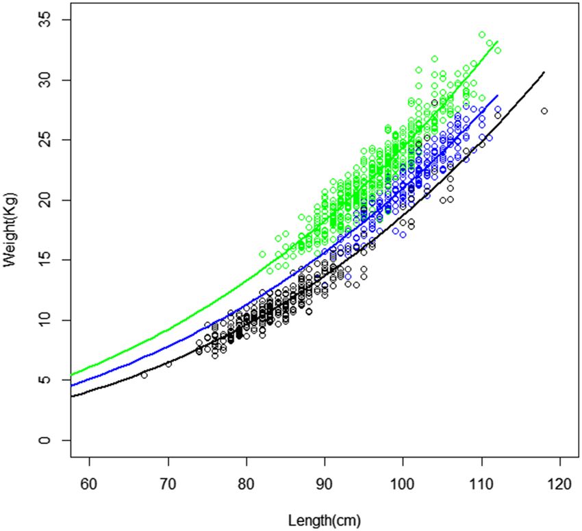
www.nature.com/scientificreports/
A common problem in fisheries research is to decide if the parameters from a simple linear regression fit are
different between p opulations53. Analysis of length–weight relationships per sampling case T1 were performed
using the R statistical software with F SA53 and M ASS54 packages. The exponential equation W = a * FLb was fit-
ted to determine the relationship between FL and W, where, a is the coefficient related to body form and b is the
exponential expressing relationship between length–weight, also called allometric coefficient55,56. Parameters
were estimated using a Nonlinear Least Squares (NLS) method from the function of R ossiter57 to provide more
2
precise relationships than the classical relations. The coefficient of determination ( R ) was used as an index of the
goodness of fit of the estimates and standard error was calculated for parameter estimations. Graphical analysis
was performed for the comparison between geographic regions with reported allometric equations.
To determine if the parameter estimates are statistically different among geographic regions, sexes and sea-
sons, the length–weight model was transformed to a linear model by taking the natural logarithms, log(Wt) = lo
g(a) + blog(FLt) + ϵt, with y = log(W), x = log(FL), slope = b, and intercept = log(a). We then determined whether
log(a) and/or b differs mainly between geographic regions and sexes using analysis of covariance (ANCOVA). A
test of whether the fish in a population exhibit isometric growth or not can be obtained by noting that b is the esti-
mated slope from fitting the transformed length–weight m odel53. The following statistical hypotheses (H0: b = 3
“Isometric growth”; ⇒ H1: b ≠ 3 “Allometric growth”) were tested using t-tests from the linear regression results.
Molecular analysis. Technical protocols. The genomic DNA was isolated from a tissue sample of muscle
(25 ng) without fat and skin using Qiagen DNeasy spin columns and quantified with NanoDrop (Thermo Fisher
Scientific).
Microsatellite PCRs were performed on selected loci (see description of the selection process in supplemen-
tary text S1-a, S2-b, and Appendix 3) in 25 μl reactions containing 5 ng of template DNA, 1X reaction buffer,
1.5 mM MgCl2, 0.24 mM dNTP, 0.1 μM of each primer, and 1U Taq polymerase. The PCR cycling for microsatel-
lite markers consisted of an initial denaturation at 95 °C for 10 min, followed by 40 cycles: denaturation at 95 °C
for 30 s, annealing at the appropriate temperature (55 °C) for 30 s, and extension at 72 °C for 1 min and a final
extension at 72 °C for 10 min. Each PCR had a negative control as well as a positive control. The PCR products
were genotyped with Applied Biosystems 3,730 XL and the profiles obtained were analysed using G eneMapper®
v5.0 software. Allele binning was performed using the bins created in the study by Nikolic et al.58 and adding
alleles respecting the allele size (± 0.4 bp). The corresponding type of repetition (e.g. di and tri) was respected
as much as possible.
Population genetic diversity and differentiation. For the purpose of this paper we define “migration” as the
movement of individuals from one place to another, “dispersal” as the process or result of the spreading of indi-
viduals from one place to another and “gene flow” as the transfer of genetic variation from one population to
another. We use the term “gene flow” when Nm (number of efficient migrants entering a population by genera-
tion) is estimated and “migration rate” when m (fraction of individuals sampled in a given group that are more
likely migrants derived from another population of origin) is estimated.
Nuclear data. Genetic analyses were performed using individuals clustered a priori according to each of the
putative stock scenarios (T1-3) (number of alleles, heterozygosity, and FIS; similar to previously described analy-
ses per marker see text S1-a). We added analysis of FIS by bootstrapping (1,000) to obtain 95% confidence
intervals (CI) with GENETIX. Hardy Weinberg Equilibrium (HWE) tests in each population and in the overall
data were carried out using GENEPOP v4.0 software59 with Markov chain parameters (10,000 dememorization,
1,000 batches, and 10,000 iterations per batch) (hypothesis Ho = random union of gametes) with an alternative
hypothesis (H1 = heterozygote deficit).The U Score test was used as it is more powerful than the probability-
test especially when there is inbreeding or population admixture60. Q-test analysis are preferable to maintain a
proper balance between the avoidance of type I errors and the induction of type II errors61–65, so we added this
analysis using Q-value R package as it performs the false discovery rate (FDR)61–65. We completed our under-
standing on deviation of HWE by using HWxtest V.1.1.9 R package66 because in most tests for Hardy–Weinberg
proportions (with real data and multiple alleles) there are often rare alleles which make the asymptotic test unre-
liable. By using the genotype counts contained within each test, we extracted and re-analysed the data to plot the
distribution with Monte Carlo sample size, for a smoother curve.
Genetic differentiation among samples within each scenario (T1-3) was estimated as pairwise Wright’s F-sta-
tistics (FST)67 using ARLEQUIN 3.168 computed with 10,000 permutations and significance level at 0.05. FST
average with 95% confidence interval (CI) and standard deviation (SD) was computed using G ENETIX69 with
1,000 bootstrap. Representation of genetic matrix distance (FST) and Principal Component Analysis on allelic
frequencies was performed using the R package A DEGENET70,71. Isolation by distance (IBD) in sampling sce-
nario T2 was tested using a Mantel test between genetic (FST and Euclidean Edwards’ distance) and geographic
distances with 10,000 resampling between individuals and geographic regions using ADEGENET, A DE472 and
GRDEVICES (R Development Core Team and contributors worldwide) R packages. Finally, IBD differentiation
(patches) was performed using a 2-dimensional kernel density estimation with MASS R package.
The hierarchical genetic structure and the admixture rates were estimated by the Bayesian individual cluster-
ing assignment performed with StRUCTURE 2.3.4 software73 with the admixture model and correlated allele
frequencies. The number of clusters, k, was determined by comparing log-likelihood ratios in 5 runs for values of
k between 1 and 14 (number of main geographic sampling + 1) with a burn-in period of 100,000 steps followed
by 1,000,000 MCMC replicates. For obtaining optimal k, results were analysed through StructureSelector74 (see
https://lmme.ac.cn/StructureSelector/) using the methods o f73,75,76, and77.
Scientific Reports | (2020) 10:15657 | https://doi.org/10.1038/s41598-020-72369-w 4
Vol:.(1234567890)www.nature.com/scientificreports/
Bifurcated evolutionary trees were built using POPTREEW78 with 100,000 bootstrapping samples and DSW
genetic distances. GenGIS 2 79 was used to build a 3D phylogeography tree with sample geographic site informa-
tion and phylogenetic tree from POPTREE280 file results. Additional analysis (AMOVA, network analysis etc.,
see supplementary text S1-b) were performed in order to check for consistency of the results when based on
different a priori.
Test for sex‑bias. We used a population assignment test for sex-biased dispersal using the software GenAlEx
v. 681. This method produces Assignment Index correction (AIc) values for each sex according to Mossman
and Waser82. Mean negative AIc values characterize individuals with a higher probability of being immigrants,
whereas positive values characterize individuals with a lower probability of being migrants. The statistical analy-
sis was carried out using the R statistical computing version 3.3.083 and included the following libraries (“law-
stat”84; “ade4”85; “mgcv”86,87; and “glmmADMB”88,89). AIc values for each sex were compared with a non-para-
metric Mann–Whitney U-test (also known as the Mann–Whitney–Wilcoxon, MWW) because samples violated
assumptions of the normality and homoscedasticity (homogeneity of variance) (Shapiro’s, Levene’s and Brown
and Forsythe’s tests).
Combining molecular and morphologic analysis. A fork length measurement was available for all but five
individuals genotyped in this work. The length–weight relationship estimated previously (Appendices 4, 5), was
used to estimate the lengths of the five fish without a length measurement. We used the assignPOP R p ackage90
to perform population assignment using a machine-learning framework and employed genetic and non-genetic
(morphometric) data sets, evaluating the discriminatory power of data collected. We tested the power of assign-
ment with 1 to 8 hypothetical populations. We used principle component analysis (PCA) for dimensionality
reduction; Monte-Carlo cross-validation to estimate mean and variance of assignment accuracy; K-fold cross-
validation to estimate membership probability; resample individuals and loci either randomly and based on
locus FST value; machine-learning classification algorithms, including LDA (Linear Discriminant Analysis) and
SVM (Support Vector Machine). The output was visualized using ggplot2 functions.
The package assignPOP was also used to standardize the data with and without the optional software to
remove low variance loci across the dataset. The default setting of variance threshold is 0.95, meaning that a locus
will be removed from the dataset if its major allele occurs in over 95% of individuals across the populations. A
low variance locus—which has a major allele in most individuals and a minor allele in very few individuals—is
not likely to be useful because an allele that only occurs in the training or test data will not help ascertain popula-
tion membership of test individuals.
Particle‑tracking simulation design. Passive drift simulations. Larvae, juvenile and young albacore
(less than 80–90 cm LF) are thought to be less able to perform vertical migration as their swim bladder is not
yet functional91 and young albacore predominantly inhabit shallow water (< 50 m)92, hence simulations of sur-
face water movements are relevant to track dispersal. Moreover, spawning takes place at the sea-surface 93,94. To
compute the trajectories of passively drifting individuals, we used the modelled surface current fields from the
GLORYS-1 (G1) reanalysis of the World Ocean c irculation95 performed by the Mercator-Ocean centre (https
://www.mercator-ocean.fr/) with the NEMO numerical ocean model (https://www.nemo-ocean.eu/). The G1
model has a horizontal resolution of 0.25° and 50 vertical layers. The G1 reanalysis provides a close-to-reality,
3-dimensional, simulation of the World Ocean dynamics as it assimilates satellite altimetry, temperature and
salinity measurements. Passive drift trajectories were computed using the Lagrangian trajectory simulation soft-
ware ARIANE (freely available at https://www.univ-brest.fr/lpo/ariane/) and the G1-simulated currents in the
first model layer (surface currents). One geographic region per day was recorded for analyses of trajectories.
This trajectory simulation technique was previously used to study the passive dispersal of hatchlings (and then
juveniles) from the west Atlantic leatherback turtle (Dermochelys coriacea) population96,97.
We chose to simulate the dispersal of particles drifting only with surface currents. Passive drift is the most
parsimonious hypothesis for exploring early stages (i.e. egg, larvae (1 month cohort) and small juveniles (three
monthly cohort) connectivity, given the high uncertainty about (1) the depth occupied and (2) the development
of swimming ability. We performed passive drift simulations over 1 month and 3 months (young of the year
individual). After the juvenile phase, fish are capable of active movement (linked to their size and habitat) in
addition to being transported by oceanic c urrents98.
Individual release. Between 1,000 to 5,000 particles were released in each simulation but for visual reasons we
presented 2000 particles in the figures. Release positions were uniformly distributed over potential spawning
regions8,36, except in the southeast Atlantic C-D (unknown spawning region in this case, including South Africa)
but it was important to test for a possible migratory pathway from SEAO to SWIO. Individuals were released
daily during a 3-month period corresponding to the spawning season. Releases are performed uniformly over
time (i.e. the same number of individuals was released every day). To address the interannual variability in the
currents, we performed 17 simulations—one per year between 1998 (first year of available current data) and
2014 (last year of the sampling program)—for each potential spawning ground. From these simulations we then
computed the average, minimal and maximal numbers of transits between the different areas.
Ethical approval and informed consent. Fish samples authors confirm that all experiments were car-
ried out in accordance with regulations. The field studies did not involve endangered or protected species. Alba-
core tuna is a commercial species all over the world that is, thus far, not subject to any ethical official rules. No
specific permissions were required for the sampling locations. Fishes were sampled from French, Seychelles and
Scientific Reports | (2020) 10:15657 | https://doi.org/10.1038/s41598-020-72369-w 5
Vol.:(0123456789)www.nature.com/scientificreports/
Regions n a Std. error (a) b Std. error (b) R2 Analysis of covariance
–5 –5 –2
A 269 5.9206 × 10 1.987 × 10 2.7747 7.259 × 10 0.8520
B 485 8.4869 × 10⁻⁵ 1.648 × 10⁻⁵ 2.7293 4.236 × 10⁻² 0.8950
–5 –6
C 302 2.0103 × 10 4.172 × 10 2.9846 4.619 × 10⁻² 0.9127
A-B 754 5.7418 × 10⁻⁴ 1.474 × 10⁻⁴ 2.3007 5.583 × 10⁻² 0.6983 Intercepts significant
A-C 571 5.1527 × 10⁻⁶ 8.293 × 10⁻⁷ 3.2983 3.507 × 10⁻² 0.9502 Intercepts significant
C-B 787 2.6044 × 10⁻⁶ 6.102 × 10⁻⁷ 3.4786 5.127 × 10⁻² 0.8719 Slopes and intercepts significant
A-B-C 1,056 1.2819 × 10⁻⁵ 2.758 × 10⁻⁶ 3.1212 4.691 × 10⁻² 0.8390 Slopes and intercepts significant
Table 1. Length–weight relationships of albacore tuna according the equation weight (kg) = a*FLb from
the non-linear least squares (NLS) form per geographic regions cases. n is the number of individuals, a the
constant, b the allometric coefficient, R2 the coefficient of determination, and Std. Error the standard error. The
last column summarizes the Analysis of Covariance (ANCOVA) with the linear model (General Linear Model,
GLM) between geographic regions.
Figure 2. Length–weight relationship (fork length (cm) and weight (kg)) for albacore (Thunnus alalunga) per
geographic regions from the catch data of Reunion (blue; region A), Seychelles (green; region B) and South
Africa (black; region C) fishery. The curves represent the length–weight relationship according to NLS form:
Seychelles (green), Reunion (blue), and South Africa (black).
South African fishing vessels (at sea with within observer program) in the authorized marine waters or at land-
ing. Only dead fish were sampled.
Results
Morphometry. Length–weight data were not normally distributed across the overall data (Lilliefors test:
p < 0.001), and the variances were heterogeneous among geographic regions (Levene test: F = 8.41, p < 0.001 for
the size; F = 13.12, p < 0.001 for the weight) and sexes (Levene test: F = 19.26, p < 0.001 for the size; F = 9.19, p < 0.01
for the weight). Univariate nonparametric statistical tests revealed that sizes and weights significantly differ
among regions (permutation test: chi-squared = 509.69, p < 0.001 for the size; chi-squared = 643.78, p < 0.001 for
the weight) and sexes (permutation test: chi-squared = 26.76, p < 0.001 for the size; chi-squared = 16.3, p < 0.001
for the weight).
Length–weight relationships in sampling scenario T1 (regions A, B, and C) revealed significant differences
between geographic regions (Table 1), with a lower ratio for individuals from South Africa (Region C), prob-
ably due to the sampling of earlier life stages, and higher values for the northernmost Indian Ocean (Region B)
(Fig. 2). The homogeneity test (ANCOVA) also revealed significant differences among geographic regions. Here
we considered estimates of length at 50% maturity around 90 cm fork length (FL)46 at an age of 4–5 years. Based
on length of adult fish (> 90 cm FL), individuals caught would therefore be considered as adults in geographic
regions A and B, and immatures in C and D (Appendix 2). For more details on the length–weight relationship
see supplementary text (S2-a).
The results indicate differences in the length–weight relationships between geographic regions (Table 1, Fig. 2,
Appendix 4). While the interaction terms are not significant between the geographic regions A and B (p = 0.1166),
Scientific Reports | (2020) 10:15657 | https://doi.org/10.1038/s41598-020-72369-w 6
Vol:.(1234567890)www.nature.com/scientificreports/
Samples n MNa He Hnb Ho FIS
Scenario T1
A 466 16.8 74.2 ± 13.0 74.3 ± 13.0 71.1 ± 12.4 0.043 (0.033–0.052)
B 466 16.8 73.9 ± 12.9 74.0 ± 12.9 71.4 ± 12.7 0.035 (0.026–0.043)
C 598 17.9 74.1 ± 13.5 74.2 ± 13.6 68.8 ± 12.4 0.072 (0.061–0.082)
D 344 16.9 74.8 ± 12.5 74.9 ± 12.5 70.3 ± 12.3 0.062 (0.050–0.071)
Scenario T2
A1 236 15.4 74.3 ± 12.8 74.5 ± 12.9 71.4 ± 12.2 0.042 (0.027–0.052)
A2 230 14.8 73.9 ± 13.2 74.1 ± 13.3 70.8 ± 13.0 0.045 (0.029–0.057)
B1 233 15.4 73.7 ± 13.2 73.9 ± 13.2 71.4 ± 13.5 0.033 (0.019–0.043)
B2 233 14.9 73.9 ± 12.8 74.1 ± 12.8 71.3 ± 12.4 0.038 (0.023–0.046)
C1 322 16.0 74.1 ± 13.5 74.2 ± 13.5 69.3 ± 12.4 0.067 (0.052–0.077)
C2 276 15.6 73.9 ± 13.6 74.1 ± 13.7 68.3 ± 13.0 0.079 (0.060–0.092)
D1 156 14.8 74.8 ± 12.8 75.1 ± 12.8 70.7 ± 13.2 0.059 (0.039–0.071)
D2 188 14.9 74.5 ± 12.4 74.7 ± 12.4 69.9 ± 12.1 0.064 (0.046–0.075)
Scenario T3
A-B 932 18.5 74.1 ± 13.0 74.2 ± 13.0 71.2 ± 12.5 0.039 (0.033–0.045)
C-D 942 19.1 74.4 ± 13.1 74.5 ± 13.1 69.4 ± 12.2 0.068 (0.060–0.075)
Table 2. Descriptive statistics for albacore samples over 32 microsatellite loci without null alleles. Number of
genotyped individuals (n); mean number of alleles (MNa); mean percent of expected (He), expected unbiased
(Hnb), and observed (Ho) heterozygosity; and inbreeding coefficient (FIS) with CI 95%. Significant values are
in bold. Mean values are ± SE. Sample abbreviations as in Fig. 1. Different samples considering scenarios of
clustering T1, T2, and T3 (sampling scenario).
and A and C (p = 0.5044) (i.e. not enough evidence to conclude a difference in slopes), the P-value (p) for the
indicator variable suggests that there is a difference in intercepts between these two pairs of geographic regions
(p < 2.2 × 10⁻¹⁶). Because these geographic regions (A and B, A and C) have statistically equal slopes but differ-
ent intercepts, there is a constant difference between the log-transformed weights of albacore regardless of the
log-transformed lengths of albacore. Concerning geographic regions B and C, there is significant difference (in
slopes and intercepts) in the length–weight relationship between the two geographic regions (p = 0.003334 and
p < 2.2 × 10⁻¹⁶ respectively).
Males are significantly larger than females (Appendix 5), except in South African waters (region C), where
most immature individuals were collected. The Appendix 5 summarizes the NLS-adjusted curve for each geo-
graphic region and the linear models to test sex-specific differences. The difference in length–weight relationship
between the sexes is significant in geographic region A. Yet, for geographic region B, the results show differences
between the sexes (Kruskal–Wallis test p < 0.05) that are not confirmed by the parallelism test (contained in the
linear model with the length–weight relationship). Females appear heavier than males for the fork length below
99 cm. This trend reverses above 99 cm fork length. However, these differences in the length–weight relation-
ship per sex in geographic region B are not confirmed by the analysis of variance (Appendix 5). A bias in sex
ratio (proportion of females to males in the sample) in favor of females with fork length (FL) < 100 cm has been
confirmed in a previous study of geographic regions A and B 36. In geographic region C, both males and females
reached smaller sizes compared to the other geographic regions, due to the dominance of juveniles in the sample.
Molecular. Genetic diversity. Descriptive statistics across loci and samples, and for each microsatellite and
sample are shown in Appendix 3. Based on the 32 microsatellite markers retained after quality selection from
the initial panel of 54 putative loci (see Supplementary text S2-b), analyses were performed considering four
different geographic groups (Fig. 1) under three a priori scenarios of individual grouping, T1, T2 and T3. Clas-
sic genetic variability per geographic group and scenario is described in Table 2. High expected and observed
heterozygosity values were found for all samples, with values ranging from 73.7 ± 13.2 to 74.8 ± 12.8 for He and
68.3 ± 13.0 to 71.4 ± 12.7 for Ho. All samples or groupings had significant P-values for Hardy Weinberg tests,
meaning that all scenarios resulted in a deficit of heterozygotes (Table 2). Inbreeding coefficients (FIS) and CI
95% were superior to 0 for all sampling locations (0.03–0.08) with the lowest values for geographic regions A and
B (particularly B1), and the highest for region C (Table 2). Overall data and each population per scenario pre-
sented a significant deviation from HWE, yet with a high proportion of False Discovery Rate (> 0.45). Based on
these results, we completed marker analysis using HWxtest. All markers presented a tail in the distribution and
17 markers also presented infrequent alleles creating a “shoulder” in the distribution. Those potential outcomes,
in which a rare genotype occurred, can partly explain the observed deviation from HWE.
POWSIM99 results for the 32 loci dataset indicated that the probability of detecting population structure
was high and statistically significant at FST ≥ 0.001 for χ2 and Fisher’s tests. When FST was set to zero (i.e. no
divergence among samples), the proportion of false significant values (α type I error) was lower than the intended
value of 4% for χ2 test and was 7% for Fisher’s test. Markers shared a similar range of mutation rates (u) of around
2 × 10⁻⁴ (mean) and 1 × 10⁻⁴ (median).
Scientific Reports | (2020) 10:15657 | https://doi.org/10.1038/s41598-020-72369-w 7
Vol.:(0123456789)www.nature.com/scientificreports/
Scenario T1 A B C D
A 0
B − 0.00005 0
C 0.00127 0.00143 0
D 0.00281 0.00340 0.00013 0
Scenario T2 A1 A2 B1 B2 C1 C2 D1 D2
A1 0
A2 0.00066 0
B1 0.00044 − 0.00030 0
B2 0.00022 0.00045 0.00038 0
C1 0.00141 0.00042 0.00045 0.00145 0
C2 0.00272 0.00101 0.00193 0.00213 − 0.00032 0
D1 0.00290 0.00287 0.00385 0.00310 − 0.00100 0.00026 0
D2 0.00290 0.00187 0.00292 0.00278 0.00024 − 0.00077 − 0.00145 0
Scenario T3 A-B C-D
A-B 0
C-D 0.00198 0
Table 3. Pairwise FST among albacore for albacore samples considering the three scenarios clustering T1, T2
and T3 over 32 microsatellite loci with 10,000 permutations. Significant corrected P-value (< 0.05) are bold.
Figure 3. (A) Mantel test correlation (the original value of the correlation between the distance matrices
is represented by the dot, while histograms represent permuted values (i.e., under the absence of spatial
structure); here the isolation by distance is clearly significant, and (B) scatterplot of isolation by distance using
a 2-dimensional kernel density estimation (red line is the correlation). Both analysis between Euclidian genetic
and geographic distances using the sampling scenario T2 (regions A1, A2, B1, B2, C1, C2, D1, and D2).
Population structure. The clustering analysis, carried out with STRUCTURE (Appendix 6), over 5 runs,
favoured the existence of two main clusters. Pairwise FST values (Table 3) were significant between almost all
comparisons of A/B with C/D, under all 3 scenarios, indicating differentiation between SEAO and SWIO Indian
samples. Pairwise FST with the scenario T2 revealed lower (and not significant) FST values between eastern
Madagascar (A2) and South Africa (C1), and also between Mozambique Channel (B1) and South Africa (C1)
(Table 3).
AMOVA results revealed significant genetic differences among the two genetic clusters (A/B, and C/D) rep-
resenting 20% of the total variation and among individuals within geographic area (A, B, C, and D) representing
36% of the total variation. The Mantel test confirmed a significant (p < 0.05) correlation between both genetic
distance (FST and Euclidean) and geographic distance (Fig. 3A, e.g. with Euclidean distance). However, the
scatterplot showed two consistent clouds of points, thus suggesting that apparent IBD was actually mostly due to
the existence of two separate entities rather than by a regular increase of genetic differentiation with geographic
Scientific Reports | (2020) 10:15657 | https://doi.org/10.1038/s41598-020-72369-w 8
Vol:.(1234567890)www.nature.com/scientificreports/
Figure 4. Schematic simulated passive drift trajectories for tuna larvae (and then small juveniles) released from
different potential spawning areas (delineated by dotted lines): East Madagascar (A), North Madagascar (B),
Southeast Atlantic (C, D), and Mozambique Channel (E).
distances (Fig. 3B, e.g. with Euclidean distance). The 3D geophylogeny Neighbour Joining (NJ) from Dsw dis-
tances (Appendices 7 and 8) also differentiated SEAO from SWIO, in line with STRUCTURE (Appendix 6), and
PCA (Appendix 9).
AssignPop analysis (Appendix 10), combining the genetics and morphometrics (length), supported the sce-
nario of two genetic clusters k = 2 (A/B, C/D). When using the genetic-morphometric data, the assignment accu-
racies of regions A and B increased and that of region C remained high, resulting in increasing overall assignment
accuracy (Appendix 10-B). Assignment accuracies of region B remained low (Appendix 10-B). The results were
similar with removal of alleles with low variance. The addition of the variable sex did not improve the results.
Test for sex‑biased dispersal. Analysis of sex-biased dispersal showed that males have strongly negative AIc val-
ues for groups A-B (southwest Indian Ocean), and C (South Africa), indicating that males are more often likely
to be immigrants (Appendix 11). Nevertheless, the Mann–Whitney U-tests were not significant.
Predicting connectivity through passive drift: particle‑tracking modelling. We chose to present
results from the simulation of the year 2009 that corresponds to a neutral phase of the Indian Ocean Dipole
(IOD)100. IOD is an oscillation of the sea-surface temperature between the eastern and western side of the tropi-
cal Indian Ocean. Similarly to the El Nino Phenomenon in the Pacific Ocean, IOD has a strong influence on the
climate-ocean system of the Indian Ocean and affects surface and subsurface c urrents101.
Simulated 1- and 3 month trajectories of passive drift are shown in Appendices 12 and 13. A schematic view of
the number of transits between the areas after 1 and 3 month drift is presented in Fig. 4. One month trajectories
display similar spatial patterns as 3 month trajectories, but 1 month is too short to draw conclusions about the
destination of the particles except for the ones released off South Africa (Appendix 12).
Modeling results suggest that connectivity through passive drift is possible, although low, between SEAO
and SWIO. Passive exchange between the southeast Atlantic (C-D) and the three potential spawning grounds
in the southwest Indian Ocean (A, B, E) appear to be highly asymmetric and subject to significant inter-annual
variability (Fig. 4). Particles released in the SEAO can be driven very quickly (within less than 1 month) into
the Indian basin by the eastward flowing Agulhas Return Current that originates from the retroflection of the
Agulhas Current off the southern tip of Africa. Over the 20 individual years tested, an average proportion
of 2.7% (min. = 1.7%, max. = 4.7%) of particles passed from SEAO to SWIO after 1 month of drift, and 4.9%
after 3 months (min. = 2.1%, max. = 6.7%). After entering the Indian Ocean particles from the Atlantic circulate
eastward around 40°S. We found no direct connectivity through early life stages between SEAO and the three
potential spawning grounds of SWIO. Particles that remained in the southeast Atlantic disperse northwestward
with the Benguela Current and the South Atlantic Equatorial Current. The passive dispersal route from SWIO
to SEAO is longer and more complex. The Mozambique Channel appeared to be the main pathway linking the
SWIO to the SEAO. Dispersal in the Mozambique Channel indicated large mesoscale activity but is mostly
southward. At the southern end of this channel, water continued to move southward with the Agulhas Current.
No particles entered the SEAO from the northern Mozambique Channel (E region) after 1 month of dispersal,
and only a small percentage entered after 3 months (mean = 0.3%, min. = 0%, max. = 2.4%).
Passive exchanges to the SEAO were predicted to be far more limited from the East of Madagascar (A) and,
surprisingly, almost non-existent from North of Madagascar (B), although located in the direct vicinity of the
Mozambique Channel. In fact, most particles from B were entrained toward the Equator line and dispersed
into the North Hemisphere. Within 1 month and 3 month of drift, no particles originating from areas A and B
were able to reach the SEAO. The A region is strongly connected with the E region, and, to a lesser extent, with
the B region, by the North Madagascar Current that flows northwestward and then goes around Cap d’Ambre,
the northern tip of the island. Passive transport from A to E accounted for 9.8% (min. = 6.5%, max. = 13.4%)
of particles after 3 months. In comparison, the B region was crossed in average by 0.4% of particles from A
Scientific Reports | (2020) 10:15657 | https://doi.org/10.1038/s41598-020-72369-w 9
Vol.:(0123456789)www.nature.com/scientificreports/
(min. = 0%, max. = 1.4%) after 3 months. Very few passive particles travelled to A region from B. Passive con-
nectivity from B to E was very weak after 3 months of drift (mean = 0.2%, min. = 0%, max. = 0.7%). The pattern
was similar in the opposite direction (from E to B), but subject to greater interannual variability: an average
proportion of 0.04% (min. = 0%, max. = 0.7%) of particles transited this way after a 3 month drift. Interestingly,
it appears that passive connectivity from E to B (northward drift through Mozambique Channel) was inversely
proportional to the passive connectivity from E to C-D (southward drift). Drift simulations from the spawning
region offshore of northwest Australia (F) indicated that passive flow from southeast to north Indian Ocean is
also possible (Appendix 13). Indeed, several particles released in this geographic region were driven westward
by the South Indian Equatorial Current.
Discussion
The results presented here indicate small but significant genetic and morphometric differences between the
southeast Atlantic and southwest Indian Oceans, suggesting the existence of two independent populations, and
identifying a spawning ground in South Western Indian Ocean waters (eastern Madagascar). We consider these
results in relation to simulations of larval dispersal through the main currents, and previous data on other species
in the same geographic region, before discussing their implications under the current delineation of management
units. The results have significant implications for RFMOs (e.g. ICCAT and IOTC) as the stock assessments and
in turn the sustainable management of albacore relies on the accurate representation of population structure
and connectivity across management units.
Instantaneous population structure based on morphometric data. Stock identification is tradi-
tionally based on morphometric differences, sometimes combined with demographic modelling. The morpho-
metric analyses of albacore tuna revealed differences in the weight, regardless of the length, between geographic
regions from SWIO waters (regions A and B). The results indicate a greater albacore weight gain in northernmost
waters, in line with previous hypotheses that the waters between the Seychelles and the coast of Somalia consti-
tutes an important albacore feeding region43. Results obtained here are consistent with the enhanced phytoplank-
ton productivity associated with the dynamic system of mesoscale eddies of the Mozambique Channel102–104 and
mid-ocean shallow banks of the Seychelles p lateau105, whereas the Mascarenes are characterised by low-nutrient
106
subtropical waters . Surface dwelling behaviour is reported for albacore of geographic regions B and C, whereas
albacore mostly occur in deeper waters in geographic region A 43. Others a uthors107 also found morphometric
differences between southwest Indian and the southeast Atlantic albacore populations and suggested that the
Agulhas current enabled the sporadic interchange of adult albacore in deep waters.
Male albacore are significantly larger than females, except in South African waters, as found in several previ-
ous studies, showing that few females of albacore tuna exceed a fork length of 100 c m46,108. This may be due to
asymptotic growth and different natural mortality between the sexes, and/or females investing more energy into
gonad development than into somatic growth. Moreover, some a uthors46,109 suggested that increased mortal-
ity would occur just after their first reproduction. Concerning the length–weight relationship, the difference
between the sexes was only significant in the east of Madagascar and Reunion waters (region A). This suggests
the presence of an important area of reproduction in the east of Madagascar, resulting in the higher weight of the
females. This result seems consistent with large catches in the southwest Indian Ocean in the waters off eastern
Madagascar110–114 and between 10°S and 25°S45, which led to assumptions of the existence of a spawning ground
in the southwest Indian Ocean by Nishikawa et al.115, and Nishida and T anaka116, also relayed by Nikolic et al.8.
A common factor among tuna species is that spawning takes place when sea-surface temperatures94 reach or
exceed 24 °C93. Spawning generally occurs throughout the year over vast areas of the Atlantic, Indian, and Pacific
Oceans and in the warm northern equatorial waters, but in higher latitudes it is restricted to the summer months
(94,117,118). Here, the adults were mainly encountered in the SWIO region, particularly east of Madagascar. These
results are consistent with histological analyses of the gonads and the investigation of the gonadosomatic index36
corroborating that spawning occurs between 10˚S and 30˚S in the east of Madagascar from October to January.
Some authors8 estimated the potential spawning area in the southwest Indian Ocean basins (also positioned
in western areas of subtropical gyres) by mapping the catch of longline fisheries. Albacore abundance in warm
waters show a seasonal peak in November–December in the SWIO region, after which the fish would migrate
to other geographic r egions8,119. These results suggest that after the spawning season some fish migrate towards
other regions.
Long term integrated population structure based on genetic differentiation. High values of
genetic diversity were observed among all sampling locations and sampling scenarios of albacore tuna. These
values are close to those previously reported for both this s pecies11,120 and bluefin tuna121–123. The positive FIS
values obtained (0.03–0.08) are within the range of those obtained in a previous s tudy120 and the confidence
intervals also differed from zero. These values reflect a bias towards an excess of homozygotes that may be due
to a technical pitfall resulting in partial allele amplification, or due to biological origin indicating departure
from random mating. A Wahlund effect (two differentiated populations that are included in a single sample)
would imply genetic structure of approximately the same level as those FIS values, whereas FST values were
much lower. The main driver of departures from HWE seem to be the presence of infrequent alleles resulting in
rare genotypes, rather than genotyping error. The low differentiation value (low FST), despite a clear dichotomy
between SWIO and SEAO (geographic regions), is not surprising, since FST is bounded by the level of diversity
(here very high); its significance is thus more meaningful than the value itself. Moreover, it is the raw number
of migrants (Nm) rather than the migration rate (m) that determines FST, thus larger populations will tend to
exhibit lower FST values.
Scientific Reports | (2020) 10:15657 | https://doi.org/10.1038/s41598-020-72369-w 10
Vol:.(1234567890)www.nature.com/scientificreports/
All statistical methods used here on a large dataset yielded similar results, indicating structural differentia-
tion of two albacore genetic groups: one identified in the southwest Indian Ocean (regions A and B) and the
other corresponding to southeast Atlantic Ocean (regions C and D). The genetic relationship between possible
SWIO and SEAO stocks has been the subject of much debate, with conflicting results found in the literature with
genetic data (e.g.120,124), a combination of blood markers and direct tagging13. Our work however agrees with
and confirms, based on a large sample of the southwest Indian and southeast Atlantic albacore population, the
results of different authors30,31,124.
Based on catch statistics, Morita22 suggested migration of albacore between two oceans off South Africa, which
could be facilitated by the strong Agulhas Current. It is possible that the connectivity is a passive migration from
the SWIO to the SEAO (through the Mozambique Channel), and an active migration in the opposite direction.
These results and scenarios are consistent with oceanographic simulations on individual dispersal, yet imply a
limited exchange, similar to the results of the genetic differentiation and clustering analysis.
The low but significant levels of genetic differentiation reported previously for albacore tuna have been
ascribed to their population characteristics, such as reproduction in the open ocean, their highly migratory
nature, and large population sizes125,126. Significant differentiation between samples A/B (SWIO) and C/D
(SEAO), based on the analysis of allelic frequencies, suggests a very small number of migrants exchanged per
generation, implying demographic independency of populations from each side of the Cape of Good Hope.
As the area of SEAO sampled by the study does not provide suitable conditions for reproduction and spawn-
ing, it might be hypothesized to support a mixed stock, with migrants from the SWIO and the Atlantic north
of the Benguela System. Genetic data from elsewhere in the Atlantic during the reproduction period would
be needed to test such hypothesis. In a previous s tudy127, bigeye tuna from distinct stocks (Atlantic and Indo-
Pacific) have been shown to be in contact around South Africa, and the distribution and mixture of fishes from
each stock seems influenced by the dynamics of the currents in that area. Population genetic structuring can be
influenced by ecological (e.g. homing behaviour) and physical (e.g. present-day ocean currents, past changes in
sea temperature and levels) factors23. Repeated glaciations and deglaciations have caused changes in sea levels,
temperatures128,129, and c urrents127 and have regularly led to changes in the distribution of marine species. Bigeye
tuna showed divergent clades, which were assumed to have been originated during the last Pleistocene glacial
maxima23. Fish population expansion during the Pleistocene has been reported in several studies130–133 and may
lead to the modification of population structure. We thus encourage continued analyses on albacore by integrat-
ing the models of the evolutionary history worldwide.
Predicted passive dispersal based on Lagrangian simulations. Lagrangian simulations support the
possibility of passive connectivity between SWIO and SEAO regions that could shape the early dispersal of
albacore populations in this part of the globe. The connectivity between the Indian and Atlantic Oceans was
suggested or demonstrated in other species of tuna (e.g. Barth et al.134), swordfish (e.g. West135), sharks (e.g. Da
Silva Ferrette et al.136), and sea turtles (e.g. green turtles137). One shall also note that passive simulations were
unable to reproduce trajectories from SEAO to the three potential spawning regions in the SWIO region, in line
with genetic data showing significant differentiation.
Offshore of the southern tip of Africa, the Agulhas Current retroflects eastward, into the Indian Ocean. The
retroflection takes the form of an unstable jet that can shed warm eddies into the Atlantic Ocean. Passive trajec-
tories from the SEAO into the SWIO rapidly reach latitudes beyond 40°S where water temperatures are relatively
low (below 15 °C), well below 24–25 °C, the preferred range of albacore eggs and larvae45,46,138,139. These are thus
unlikely to survive. Conversely, individuals carried from the SWIO into the SEAO by the warm Agulhas Current
and then the Agulhas Rings would have a much better chance of survival due to higher temperatures than the
ones following the opposite direction to the cold Circumpolar Current, which may explain the asymmetry of
predicted passive exchange. In fact, the Mozambique Channel appears to be the only path tested where links may
occur between the southwest Indian and the southeast Atlantic Oceans. Nevertheless, according to simulations
over the duration of 1 to 3 months, connectivity is still predicted as very limited. Thus, the warm Agulhas current
may promote passive or quasi-passive dispersal of early stage albacore from the SWIO to the SEAO regions, yet
both prediction through modelling and inference through genetic data suggest this dispersal pattern, if it exists,
would be very limited. In the yellowfin tuna, an asymmetric migration was supported from the Indo-Pacific to
the Atlantic134,140, and several Indian Ocean migrants were detected at the Atlantic spawning site demonstrating
asymmetric dispersal140, as is suggested here by modelling of albacore tuna.
Large ocean currents and physicochemical characteristics are congruent with the differentiation and con-
nectivity between albacore of southeast Atlantic and southwest Indian Oceans. Predicted dispersal patterns
reported here are indeed in line with the dichotomy observed with both morphometric and genetic data. How-
ever, no obvious parameter prevents migration of post-larval or adult albacore with partially or fully developed
thermoregulation abilities from the south Atlantic to the south Indian Ocean, or the other way round. In the
southeast Atlantic adult albacore are caught down to 55°S by fisheries141. Moreover, several authors (e.g. 110,124),
using catch rate statistics, have suggested that exchange of immature fish between the two oceans may occur
during the austral summer. The Agulhas current might act as a facilitator of the transport of individuals from
SWIO to SEAO. For the passage from SEAO to SWIO, the temperature should act as a barrier to young of the
year albacore. On the other hand, adult individuals have larger temperature tolerances (between 14 and 21 °C, all
oceans and information c ombined142–149), and be able to migrate from SEAO to SWIO. Yet, genetic analyses do
not suggest a high level of migration, despite the apparent lack of physical barrier, such as in the case for bigeye
tunas that are prevented from mutual penetration between Atlantic and Indo-Pacific127.
Scientific Reports | (2020) 10:15657 | https://doi.org/10.1038/s41598-020-72369-w 11
Vol.:(0123456789)You can also read