Covid reallocation of spending: The effect of remote working on the retail and hospitality sector
←
→
Page content transcription
If your browser does not render page correctly, please read the page content below

Department
                    Of
                    Economics

Covid reallocation of spending: The
effect of remote working on the
retail and hospitality sector
Gianni De Fraja, Jesse Matheson, Paul Mizen, James
Rockey, Shivani Taneja, and Gregory Thwaites

Sheffield Economic Research Paper Series

SERPS no. 2021006

ISSN 1749-8368

02 December 2021
Covid reallocation of spending: The effect of
 remote working on the retail and hospitality
                    sector.*
 Gianni De Fraja1 , Jesse Matheson2 , Paul Mizen1 , James Rockey3 ,
            Shivani Taneja1 , and Gregory Thwaites1

                     1
                       School of Economics, University of Nottingham
                     2 Department of Economics, University of Sheffield
                   3 Department of Economics, University of Birmingham

                                 December 2, 2021
                                        Abstract
           A defining economic outcome from the Covid-19 pandemic is the un-
      precedented shift towards remote working from home. The extent and du-
      ration of this shift will have important consequences for local economies
      and especially the retail and hospitality sectors which depend on business
      around the workplace. Using a new bespoke, nationally representative sur-
      vey of UK working age adults we analyse their ability and willingness to
      work remotely, and the consequences for spending on food, beverages, re-
      tail and entertainment around the workplace. We establish five key facts.
      (i) The post-pandemic change will be large: the fraction of work done from
      home will increase by 20 percentage points over its pre-pandemic level.
      (ii) The Dingel-Neiman (2020) assessment of remote working potential by
      occupation are reasonably predictive of what workers and employers ex-
      pect to do, with a correlation coefficient of over 0.7. (iii) Relocation will be
      higher for better paid professional occupations, which will skew spending
      toward the most socio-economically affluent geographical areas. (iv) The
      corresponding geographical shift in annual retail and hospitality spending
      will be £3.0 billion with more remote working shifting demand away from
      urban areas. (v) On average, a 1% change in neighbourhood workforce
      changes local spending by 0.25%.
Keywords: Covid-19, work-from-home, local labour markets
JEL Classifications: R12, J01, H12
   * We gratefully acknowledge funding from the Economic and Social Research Council (ESRC
grant number ES/P010385/1 and ES/V004913/1).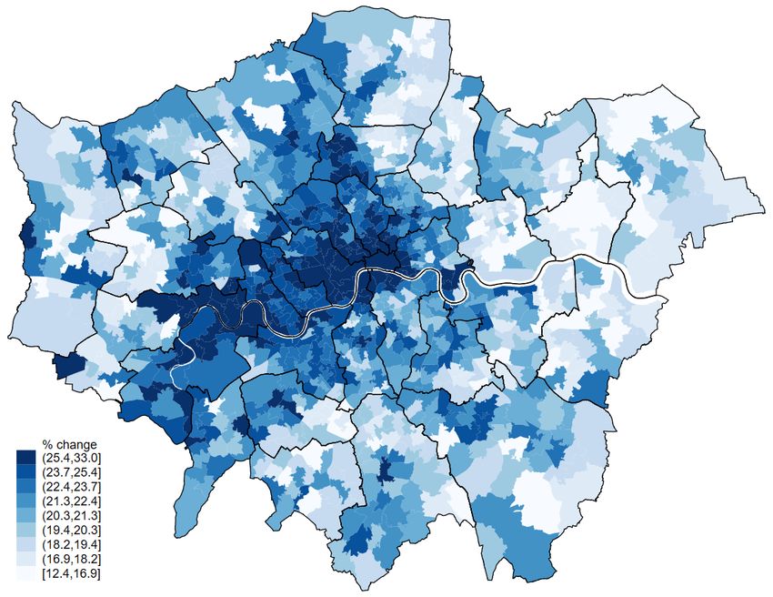
1     Introduction
The Covid-19 pandemic has had a dramatic impact on the way we work. At its peak approx-
imately 40% of all work done across England and Wales was done from home (Kent-Smith,
2020). As homeworking mandates are relaxed, there is uncertainty about how much work will
be done remotely in the medium term, by whom, and where. Firms have invested in capital
and developed patterns of working that may cause remote working (RW) to persist beyond the
point when it is necessary or required for public-health reasons. These choices will affect other
workers and business who are not party to them, and in particular those who provide locally-
consumed services (LS) such as retail and hospitality to workers who will now be working
elsewhere.
    This paper uses information from a new bespoke, nationally representative survey of UK
workers to quantify their expectations of how much they will work in the office and how much
remotely in 2022 and thereafter. We combine this with information about their occupation and
geographic location, along with their reported pre-pandemic work-related expenditure on LS
analyse to calculate occupation- and location-specific spending and shares of work done from
home, to which we apply the methodology described in De Fraja et al. (2021) to estimate ge-
ographic shifts in work and spending due to RW across England and Wales. We use this to
establish five facts about RW and its geographic and industrial impact.
    First, respondents report that the post-pandemic increase in RW will be large: the fraction
of work done remotely will increase by 20 percentage points over pre-pandemic levels. This is
similar to the estimated increase in the U.S. Barrero et al. (2021) and prior estimates for the UK
Casey (2021).
    Second, the pattern of WFH across occupations turns out to be broadly consistent with
the predictions made in Dingel and Neiman (2020): the correlation across our 25 occupational
groupings is 0.73. Workers expect to RW slightly more than thought possible in low-RW occu-
pations according to Dingel and Neiman (2020), and slightly less in high-RW occupations. Our
data provide an additional and complementary source for researchers who need to quantify
occupations by their ability to RW.
    Third, the incidence and impact of RW will vary a great deal across geographic areas. For

                                                1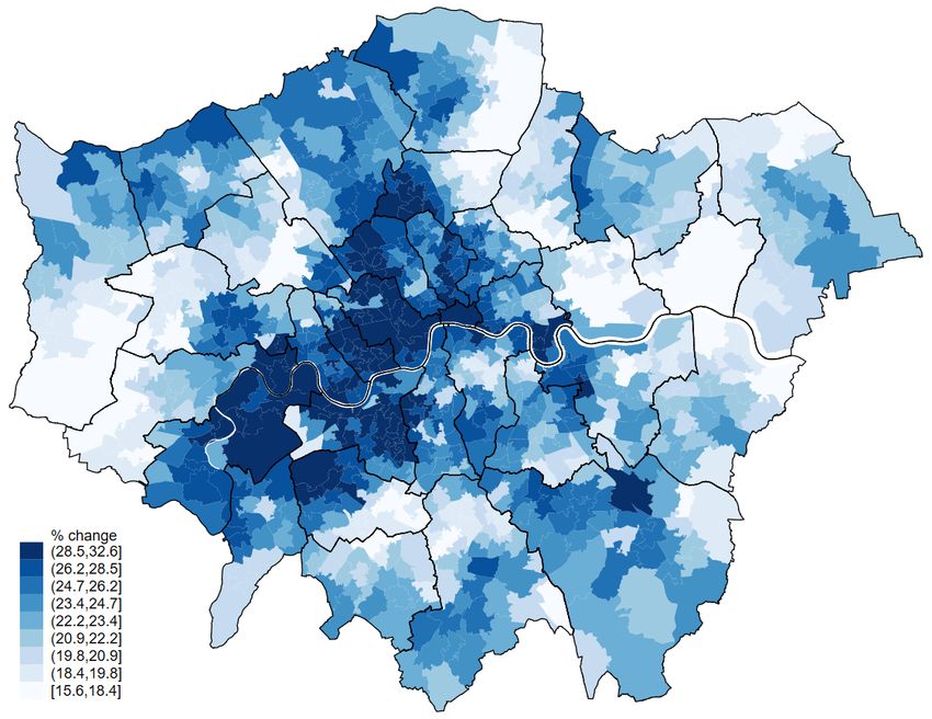
example, the increase in RW will affect city centres especially hard and most of all Central
London. There are a number of factors driving this pattern. A key factor is that where people
work is more geographically concentrated than where people live. This is especially true for
jobs that can potentially be done from home which tend to cluster in dense city centres. We also
show that workers who can work from home are likely to be relatively well-paid, resulting in a
skewing of work done from home towards more affluent neighbourhoods. Another important
factor, as our survey shows for the first time, workers’ propensity to work from home within
given occupations depends on where they live. For example, workers business management or
professional occupations who live in smaller cities and towns anticipate less RW in the future
than their counterparts who live in London or other large cities in England and Wales.
    Fourth, we estimate that around £3.0 billion in annual retail and hospitality spending (1.5%
of total spending1 ) may relocate away from urban centres to residential areas. By changing
where we spend our time, RW also changes where our spending on locally consumed services—
such as coffee shops, restaurants, and retail—takes place. The local impact of this change will
vary a great deal, with spending falling by as much 32.5% in the City of London, but potentially
increasing by more than 50% in many residential neighbourhoods. This shift in spending is
important; we estimate approximately 77,000 jobs in retail and hospitality will either need to
similarly relocate or be lost all together.
    Fifth and finally, we use these estimates to calculate the elasticity of retail and hospitality
spending with respect to a change in the neighbourhood workforce. On average, we find that
a 1% increase in person-days spent RW in a neighbourhood will lead to a 0.25% change in
spending. This estimate is consistent across different neighbourhoods in England and Wales,
but notably higher in a few neighbourhoods, such as the City of London or Canary Wharf,
where worker spending is a very large portion of overall spending on local services.
    This paper builds on a emerging literature studying the dramatic increase in RW during,
and after, the pandemic. Relative to this literature, our paper makes contributions in four
broad broad areas. First, we complement the early judgement-based assessments (Dingel and
Neiman, 2020) and surveys (Adams-Prassl et al., 2020) of different occupations’ suitability for
   1 Percentage   is based on total spending for industries working in hospitality, retail, and
wholesale.

                                                2
RW, with workers’ own expectations for the future based on their experiences over 9-18 months
of the pandemic. Second, we show that there are systematic differences in these metrics by ge-
ography as well as occupation. Third, our estimates of where work will be done across the UK
update De Fraja et al. (2021) for the UK and complement Ramani and Bloom (2021), Althoff et
al. (2021) and Brueckner et al. (2021) for the US. Fourth, we assess the externalities these moves
will have for LS in the UK, a country with a very different economic and human geography to
the US (Barrero et al., 2021).
    The remainder of the paper is structured as follows. Section 2 provides the details on how
we quantify neighbourhood-level changes in work and spending. This section also provide
details on the data sources used in this study. Section 3 presents the main results of this study
on post-pandemic remote working, retail and hospitality spending, and the implied elasticity
of local services spending with respect to remote working. Section 4 we discuss some of the
consequences of these changes for the broader economy and policy recommendations. Section
5 concludes with some implications that these results have for post-pandemic recovery policy.

2     Quantifying the geographic effect of RW
This section proceeds as follows. First, in section 2.1 we introduce and describe our survey data
on historic and expected RW and individuals’ expenditure when at work. Then, we use it to
assess differences in actual RW patterns from those predicted at the beginning of the pandemic.
Next, we study geographical regularities in RW and expenditure patterns vary by location.
Section 2.2 describes the method by which we combine the survey data with Census data to
compute, for each neighbourhood, changes in RW and retail and hospitality spending.

2.1     The Work From Home Survey
Our primary data source is the novel UK Work From Home Survey. The survey has been col-
lected monthly from January 2021, providing a sample of approximately 2,500 completed sur-
veys in each month. We work with data collected from March 2021—when data on 2019 work
patterns were first collected—up to and inclusive of November of 2021, for a total of 22, 554

                                                3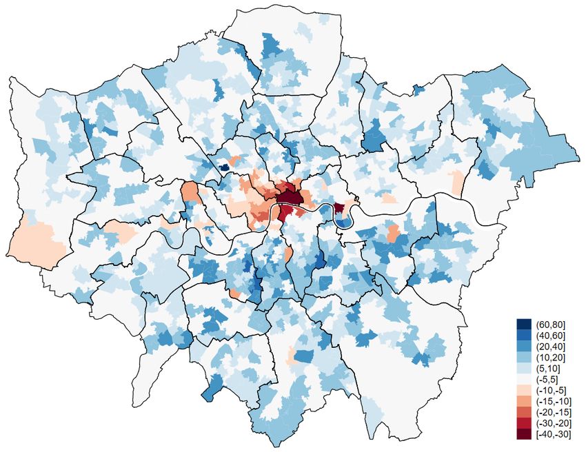
Table 1: Work From Home Survey descriptive statistics
                                                        Unweighted       Weighted
             Variables                                  Mean   SD       Mean    SD        N

             Female (%)                                 62.64   48.38   57.64   49.41   22,554
             University education (%)                   63.73   48.08   39.39   48.86   22,554
             Work income in 2019 (£’000s)†              29.57   19.54   28.06   18.93   22,554
             Days per week worked from home in 2019      0.49    1.18    0.48    1.18   22,554
             Did not work in reference week (%)         11.76   32.22   14.14   34.84   22,554
             Full days worked in reference week          3.92    1.70    3.79    1.79   22,554
             Days worked from home in reference week⋆    2.91   2.05     2.64    2.10   19,901

      Notes: This table reports summary statistics for the Work From Home Survey
      (March–November 2021). Column SD reports standard deviations for the sample.
      Weighted estimates are weighted by age, sex and education to match the Quarterly
      Labour Force Survey.
      † Income groups reported, mean is calculated based on the midpoint for each group.
      ⋆ Days worked from home are conditional on working in the reference week.

observations. The survey samples UK residents, age 20–65 who earned at least £10, 000 in 2019,
roughly corresponding to the population of adults in full-time employment. The Work From
Home Survey includes a number of results about individuals’ RW preferences, their ability to
do so, and the impact upon their productivity of pandemic induced additional RW.2 . We re-
port selected summary statistics in Table 1. For the period covered by the survey, the average
worker was working 2.64 full days per week at home (of an average 3.79 days worked in total),
compared to an average of 0.46 days per week in 2019.
    In this study we are interested in estimating the permanent shift in work done from home,
once firms and or government are no longer mandating or permitting RW for public health rea-
sons. For this purpose we focus on information about survey respondents’ belief about their
employers plans for future working arrangements to estimate working from home moving for-
ward. Specifically we look at the answer to the following survey question:

       Q1: After COVID, in 2022 and later, how often is your employer planning for you to work
       full days at home?

In the case of respondents who are self-employed (10% of the sample), we use the question

       Q2: After COVID, in 2022 and later, how often would you like to have paid workdays at
       home?
   2 Productivity   and preference results for earlier waves of the survey are reported in Taneja et
al. (2021)

                                                    4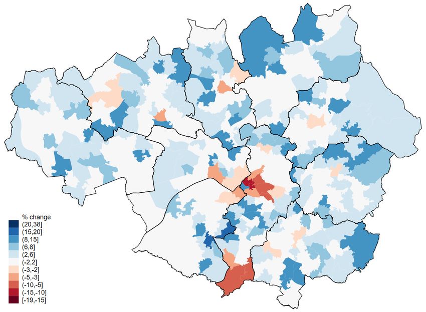
Table 2: Remote working and spending by occupation

                                                      Work done from home (%)   Spending (£)    N
                                                     in 2019   2022 over 2019   at work 2019
Armed forces                                          11.71          3.13           38.15       48
                                                      (3.53)        (4.89)          (7.83)
Construction and extraction                            3.77         10.64           38.16      161
                                                      (1.20)        (2.05)          (3.97)
Farming, fishing, and forestry                        13.71          5.50           55.18       65
                                                      (3.80)        (3.29)         (11.38)
Management, business and financial                    15.82         31.03           36.00      2,043
                                                      (0.68)        (0.82)          (0.99)
Office and administrative support                     11.38         25.34           23.98      2,593
                                                      (0.56)        (0.75)          (0.60)
Production                                             5.05         10.88           27.24      331
                                                      (1.04)        (1.48)          (1.92)
Professional and related                              24.78         25.70           31.52      1,165
                                                      (1.10)        (1.15)          (1.30)
Sales and related                                     15.53         13.36           30.83      1,258
                                                      (0.95)        (0.97)          (1.11)
Service occupations                                   10.40         11.40           28.87      622
                                                      (1.16)        (1.34)          (1.49)
Transportation and material moving                     3.02          6.20           17.89      381
                                                      (0.76)        (1.24)          (1.51)
Education, training and library                        7.59          9.23           19.98      1,939
                                                      (0.53)        (0.69)          (0.79)
Public sector                                          8.42         24.53           22.55      1,142
                                                      (0.64)        (1.00)          (0.85)
Computer and mathematical                             22.88         36.90           29.97      863
                                                      (1.25)        (1.38)          (1.49)
Architecture and engineering                           9.26         24.98           26.34      199
                                                      (1.80)        (2.35)          (2.54)
Physical and social science                           10.38         17.06           24.84      122
                                                      (2.30)        (3.29)          (2.39)
Community and social service                          12.73         23.49           26.16      253
                                                      (1.91)        (2.49)          (2.34)
Legal                                                 12.27         31.98           41.52      238
                                                      (1.76)        (2.40)          (3.09)
Arts, design, entertainment, sports, and media        36.17         20.41           31.03      738
                                                      (1.64)        (1.57)          (1.70)
Healthcare practitioner and technical                  6.12         12.04           27.99      642
                                                      (0.73)        (1.09)          (1.82)
Healthcare support                                     5.63          8.87           25.81      493
                                                      (0.91)        (1.28)          (1.49)
Protective service                                     1.18         11.35           32.97       71
                                                      (0.63)        (3.31)          (4.52)
Food preparation and serving                           3.72          7.61           30.87      252
                                                      (1.11)        (1.45)          (2.47)
Cleaning and maintenance of buildings and grounds      4.59         12.28           16.18       90
                                                      (1.87)        (2.88)          (2.52)
Personal care and service                             14.59         10.53           25.67      149
                                                      (2.83)        (2.68)          (2.91)
Installation, maintenance and repair                   8.49         14.08           18.92      122
                                                      (2.35)        (3.07)          (2.18)

Notes: This table reports remote work and retail and hospitality spending in 2019
and 2022 by occupation, calculated from the Work From Home Survey. Standard
error of mean values reported in parenthesis.

                                                 5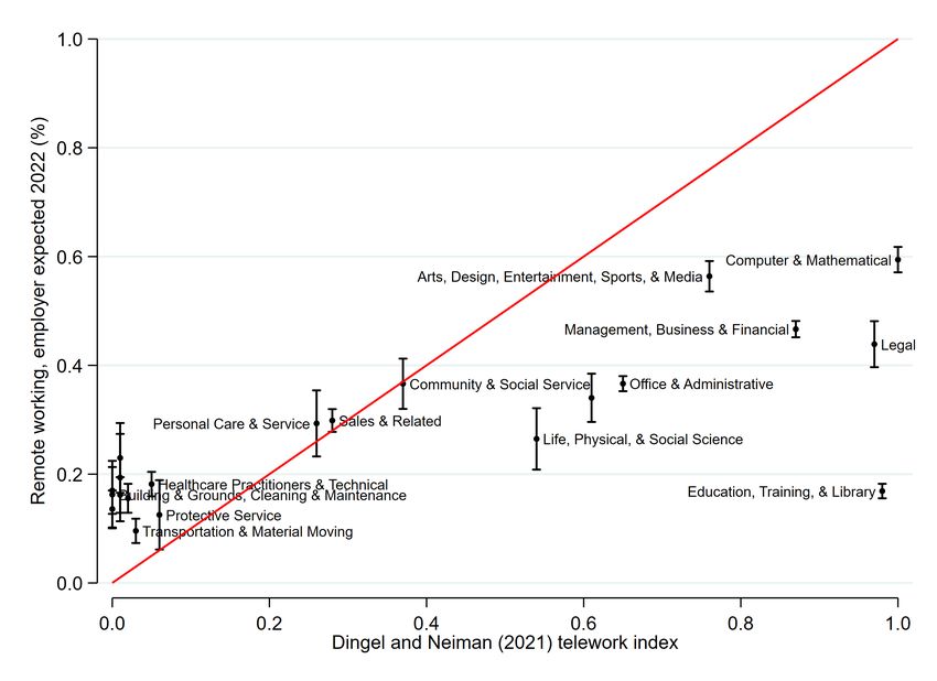
The answers to these questions are given in days, beginning with a) Never, b) About once or
twice per month, c) 1 day per week,. . . , g) 5 or more days per week. We transform responses
to each of these questions are into a share of a 5-day work week. For example, if a respondent
chooses About once or twice per month, then they are doing 10% of work from home each week;
if a respondent chooses 5+ days per week, then doing 100% of work from home each week.
    To be conservative we rely on estimates using respondents’ beliefs about their employer’s
preferences for RW rather than their own. The average respondent reports (for Q2) that they
would prefer to work from home 50% of the time—considerably higher than the average 33%
reported for Q1 above. Notice that both of these reported values are considerably larger than
the average 12% of work done from home reported for 2019.3
    The Work From Home Survey also provides information on the reported amount of spend-
ing on retail and hospitality that workers did while working at the office pre-pandemic. This is
based on the answer to three questions:

           Q3: In 2019, when you worked at your employer’s business premises, roughly how much
       money (in pounds) did you spend during a typical working week on food and drinks (e.g.
       lunch, coffee, snacks, etc.)?
       Q4: In 2019, when you worked at your employer’s business premises, roughly how much
       money (in pounds) did you spend during a typical working week on shopping near work
       (e.g. gifts or clothes shopping during your lunch break of after work.)?
       Q5: In 2019, when you worked at your employer’s business premises, roughly how much
       money (in pounds) did you spend during a typical working week on bars, restaurants, and
       other entertainment venues that are near your workplace?

The answers for each of these questions are reported in pounds.
    In Table 2 we report estimates of RW and spending while at work across the twenty-five
occupation categories recorded in the survey. As we would expect, there are considerable dif-
ferences in expected future RW. For example, office and administrative support workers are
expected to do 25 percentage points more work from home in 2022 than the 11% done in 2019.
Work in education, on the other hand, is expected to do only 9 percentage points more work
   3 The    proportion of work done from home in 2019 is a derived measure. See Appendix A for
details.

                                                    6
Figure 1:
                                                                               Remote working, 2019 and 2022

                                                             60                                                  Computer & Mathematical

                Remote working, employer expected 2022 (%)                                                                                     Arts, Design, Entertainment, Sports, & Media

                                                                                                                      Professional & Related

                                                                                                   Management, Business & Financial
                                                                                           Legal

                                                             40
                                                                             Office & Administrative
                                                                                            Community & Social Service

                                                                                                  Sales & Related
                                                                                       Life, Physical, & Social Science

                                                                                       Service Occupations
                                                             20
                                                                               Healthcare Practitioners & Technical
                                                                                 Education, Training, & Library

                                                                      Protective Service
                                                                           Food Preparation & Serving
                                                                         Transportation & Material Moving

                                                             0
                                                                  0                                     20                                         40                                         60
                                                                                                        Remote working, actual 2019 (%)

      Notes: This figure plots the expected percent of work done at home in 2022 against
      the average percent of work done at home in 2019. The 45◦ line is shown in red.

from home in 2022 than the 7.5% done in 2019. A general pattern emerges where occupations
that had higher RW rates before the pandemic both have higher RW rates after the pandemic
and have a larger incremental increase (see Figure 1)
    This variation in RW is likely driven, in part, by occupational differences in how amenable
jobs are to teleworking. We examine this by looking at the correlation between the change in
post-pandemic RW and the teleworking index reported in (Dingel and Neiman, 2020) for the
same occupations4 . We show a scatter plot of the correlation in Figure 2. The correlation of 0.78
is substantial, consistent with the teleworking index being a good predictor of future working
from home. Moreover, the differences between predicted RW and actual RW are themselves
revealing. Dingel and Neiman (2020) underestimates the potential for RW at the bottom of the
RW distribution, in occupations such as transportation or healthcare, and overestimated it at
the top-end in occupations like legal services. This highlights a key difference in these two
   4 In
      Appendix A we do the same analysis using the (De Fraja et al., 2021) adaptation of the
(Dingel and Neiman, 2020) teleworking index for UK SOC codes.

                                                                                                                          7
Figure 2:
                2022 remote working rates versus teleworking index

     Notes: This figure show a scatter plot of work from home rates by occupation as
     predicted by the Work From Home Survey against work from home indices reported
     in Dingle and Neiman (2021)— the correlation coefficient is 0.78. Vertical bars show
     95% confidence intervals for the survey estimates. The 45◦ line is shown in red.

measures, the index reflects how much work can be done from home, while we estimate how
much work will be done from home. An occupation where we see a stark difference between
the teleworking index and WFH prediction is education. This fits with the anecdotal experi-
ence throughout 2020 and 2021; although children can be educated remotely, there is a strong
preference (both from parents and teachers) to continue this work face-to-face. Likewise, while
it seemed logical that healthcare needs to be done in person innovation and adoption of new
technologies have enabled a substantial proportion of care to be done remotely.
    We now turn to our data on spending while at work. We also see considerable variation in
working from home and spending across different geographic areas. We consider four levels
of geography: Outer London, Central London5 , Other large cities, All other cities and towns. We
   5 Wedefine Central London to be the local authorities of Camden, Islington, Kensington and
Chelsea, Lambeth, Southwark, Westminster, City of London, Greenwich, Hackney, Hammer-
smith and Fulham, Lewisham, Tower Hamlets, and Wandsworth.

                                               8
Table 3: Remote working and spending by work location
Work done from home (%) Spending N
in 2019 2022 over 2019 at work 2019
Other towns and cities 12.79 17.48 24.82 11,782
(0.27) (0.33) (0.34)
Large cities (top 15 by population) 10.41 26.68 30.39 2,574
(0.50) (0.70) (0.73)
Central London 10.37 28.43 51.24 1,160
(0.72) (0.93) (1.52)
Outer London 25.24 30.00 42.17 552
(1.57) (1.51) (2.07)
Notes: This table reports work from home and retail and hospitality spending in
2019 and 2022 by location of work (in 2019). Standard error of mean values reported
in parenthesis.
define Other large cities as the fifteen largest local authorities outsides the Greater London area.
Aggregate statistics for working from home and spending are reported in Table 3. We see that
the change in working from home is considerably larger in central and outer London than in
cities and towns outside the London area. Further, weekly spending while at work is twice as
high in central London (£51.24 per week) than in smaller towns and cities (£24.82 per week).
Within several occupations we see large and significant RW variation across the different
geographic regions (see Table A1 in Appendix A). For example, a worker in office and adminis-
trative support is expected to increase their RW by 26.8 percentage points if they are in a small
local authority, compared to to 39.7 percentage points in central London. Workers in profes-
sional occupations are expected to increase their RW by 21.0 percentage points in a small local
authorities, but 36.9 percentage points in Central London. We see similarly large geographic
differences in management, legal, and healthcare. For most occupations in which there is a
large overall change in working from home, the change is expected to be largest in the London
area (an interesting exception to this is computer and mathematical occupations where we see
lower incremental RW in London versus other parts of England and Wales).
92.2 Calculating the geographic shift in working and spending
To measure how RW will affect the geography of productive activities and the resulting demand
for local services, we build on the work of De Fraja et al. (2021). They introduce what they term
as a zoomshock, the geographic change in economic activity due to the shift towards RW during
the Covid-19 pandemic. The zoomshock reflects the difference between the number of workers
who live in a neighbourhood, and can work remotely, and the number of workers who work in
a neighbourhood, and can work remotely:
Number of workers who live Number of workers who work
in neighbourhood z and − in neighbourhood z and (1)
can work remotely can work remotely
In this paper we modify this measure to reflect the amount of post-pandemic RW that we
expect to be done from home over what was done pre-pandemic. Specifically, we will compare
expectations of the amount of work that will be remote in 2022 to estimates of the amount of
RW in 2019. That is, we estimate the change in the amount of work done in a neighbourhood z
as:
∆Ez = ∑[( RWo,z
2022 2019
− RWo,z R
) Eo,z 2022
− ( RWo,z 2019 W
− RWo,z ) Eo,z ], (2)
o
2022 is the expected proportion of RW in 2022, for occupation o and neighbourhood
where RWo,z
2019 is the proportion of RW in 2019, for occupation o and neighbourhood z; E R and EW
z; RWo,z o,z o,z
are the number of workers with jobs in occupation o who live and work in neighbourhood z
(pre-pandemic).
By changing where workers are spending their time, the increase in RW will also lead to
a geographic change in where workers do their work-related spending on locally consumed
services, particularly retail and hospitality. The demand for coffees, drinks, sandwiches and
retail shopping during lunch breaks, will be shifted from neighbourhoods in which workers
work to neighbourhoods in which workers live.
We calculate this expected change in local retail and hospitality spending by weighting the
geographic movement of work across different occupations by the average spending in each
10occupation and location. Formally the change in retail and hospitality spending in a given
neighbourhood, ∆Sz , is calculated as:
∆Sz = ∑[( RWo,z
2022 2019
− RWo,z )Spend2019 R 2022 2019 2019 W
o,z Eo,z − ( RWo,z − RWo,z ) Spendo,z Eo,z ] (3)
o
Spend2019
o,z is the average spending, while at work, by workers in occupation o working in neigh-
bourhood z before the pandemic.
We use the information from the Work From Home Survey, described above, to estimate
2022 , RW 2019 , and Spend2019 in Equation (3). For each of the twenty-five survey
values for RWo,z o,z o,z
occupation categories and four location described above, we calculate the average increase in
WFH for 2022 over 2019, and the average work-related spending on retail and hospitality.
The 2011 population Census, published by Office for National Statistics, provides us with
R and
the pre-pandemic distribution of residents and workers by occupation and location, Eo,z
W . These data provide, for every middle super output area (MSOA)6 , a count of the number
Eo,z
of employees working in the MSOA by three-digit Standard Occupational Classification (SOC),
and a count of the number of employees living in the MSOA by four-digit SOC. To match with
the survey information, each SOC code is allocated to one of the 25 occupations (see data ap-
2022 , RW 2019 , and Spend2019 are assumed to be
pendix for more details), average values of RWo,z o,z o,z
constant across MSOAs (z) within each of the four geographic regions we consider above. This
means that cross MSOA variation in average spending and RW within one of the four geo-
graphic regions will be driven by variation in occupation composition.
We express both eq. (2) and eq. (3) as percentage changes. For eq. (2) this is done by dividing
by the total pre-pandemic number of jobs done in neighbourhood z. For eq. (3) we divide by
the total retail and hospitality spending for neighbourhood z. We calculate total spending for
a neighbourhood z as the total employment in retail and hospitality done (by workers and
all other forms of spending) in the neighbourhood multiplied by the output per worker. Full
details of calculations and data sources are available in Appendix A.
There are three assumptions underlying eq. (3) that are worth highlighting. First, this
6 AnMSOA is an official geographic unit used in England and Wales. Each unit defines a
geographic area in which approximately 8, 254 people reside. There are 7, 201 MSOAs across
England and Wales
11measure reflects the change in spending that will occur in each neighbourhood when work-
ers spending in 2019 is reallocated to different neighbourhoods. While a decrease in spending
is likely to be realised when workers leave city centres, where many local services are avail-
able, the corresponding increase may not be realised in residential neighbourhoods if relatively
few of such services are available (discussed in more detail in Section 4). For this reason, we
interpret ∆Sz as the geographic shift in desired retail and hospitality spending by workers.
Second, we assume that desired spending on retail and hospitality does not change when
workers work remotely as opposed to working in an office. It is plausible that when workers
work from home, with access to a full kitchen, desired spending on food and beverages de-
creases. However, it could also be that desired spending increases, as coffee shops and restau-
rants provide a valuable respite from the social isolation of home working. Likewise, some may
prefer to work remotely from cafes or hotels. For this reason, our results reflect the conservative
assumption that desired spending is independent of where work takes place. This means that
local spending will not be affected by the place of work for workers who work and live in the
same neighbourhood. If this is violated it will likely lead us to under-estimate any aggregate
decline in spending due to RW.
Third, we assume that spending is spread evenly throughout the week. This means that
working from home two days a week will result in two days’ worth of spending that does not
take place in the city centre. This may lead us to over or under-estimate the effect of home
working on spending if spending is concentrated around certain days of the week. This is
unlikely to apply to spending that is done on a daily basis, such as coffee and sandwiches, but
may be important for spending that is concentrated, as may be the case with Friday evening
drinks or retail shopping.
3 Results
In this section we present our results quantifying the geographic shift in where work is done
and the corresponding shift in desired retail and hospitality spending. We then use these results
to calculate the elasticity of spending (LS-elasticity) with respect to a neighbourhood’s change
12in work.
3.1 The geography of remote work
Computing eq. (2) for England and Wales as a whole suggests that an additional fifth (18%)
of all work will be worked remotely in 2022 compared to 2019. However, this overall figure
masks considerable variation. Figure 3 plots the estimated increase in RW by local authority as
a percentage of the total local authority workforce. Looking at the map it is clear that the change
is largest in Central London, and more generally in the remainder of South East England. We
can also see that a similar pattern is evident for other large cities, with Birmingham, Cardiff,
Leeds, and Manchester all discernible as darker patches of the map. Likewise, areas far from
major cities such as the majority of Wales, are paler reflecting lower rates of RW.
Looking at the quantile definitions in the legend makes clear another important feature of
the change in RW. The distribution of changes is heavily right-skewed. At the local author-
ity level the minimum increase in RW is 14.3% (Richmondshire District in North Yorkshire).
But, across the country the minimum increase in RW is still nearly an additional day per week
suggesting that RW is not merely an urban or suburban phenomenon. The largest increases,
29.9% for the City of London/Westminster and 29.0% for Tower Hamlets, are consistent with
an average increase of 1.5 days per week working from home.
While the average increase in RW in all London Boroughs is large, there is considerable
variation at the neighbourhood level. Figure 4 plots the estimated increase in RW at the neigh-
bourhood (MSOA) level for Greater London.7 As should be expected the average increase for
London is higher than for England and Wales as a whole. Again, the increase is right-skewed—
every London neighbourhood will see an increase in RW of at least 15.6%.
More loosely, there is evidence of a ‘doughnut’ type pattern with increases in RW highest in
central MSOAs but with higher rates in the outermost neighbourhoods than those in between.
There are many exceptions to this (e.g. the prosperous areas of West London along the river
Thames have higher rates than those further West), reflecting the complexity of London’s eco-
7 Thisfigure plots the changes in RW for residents living in each MSOA. Figure B6 in the
Appendix additionally plots the increases as a percentage of those working in each MSOA.
While there are some interesting differences, the overall implications are the same.
13Figure 3:
Change in remote working, England and Wales
Notes: This figure shows the change in working from home in 2022 over 2019, as a
percent of total local authority workforce. Boarders denote travel to work areas.
14Figure 4: Change in remote working, Greater London
Notes: This figure shows the change in the number of residents working remotely in
2022 over 2019, as a percentage of total neighbourhood (MSOA) workforce. Boarders
denote local authorities.
nomic geography. Nevertheless, excepting these nibbles, overall the doughnut pattern is clear.
Of course, this pattern is not a coincidence but reflects differences in affluence, workers living in
more affluent neighbourhoods are more likely to have jobs that allow for hybrid working. This
doughnut pattern is similar in spirit, if not detail, to the ‘donut effect’ identified by Ramani and
Bloom (2021).8
3.2 Change in retail and hospitality spending
We now turn to the change in spending. Calculating eq. (3) for the entirety of England and
Wales suggests an aggregate geographic reallocation of desired retail and hospitality spending,
as a result of the post-pandemic increase in RW, of £3.0 billion. This is approximately 1.5% of
8 Ramani and Bloom (2021) provide evidence of a migration amongst those able to RW from
the centre of major US cities to their suburbs, and a consequent change in rents. There the donut
refers to the suburbs with the central business district the hole, here, the doughnut refers to an
inner ring of suburbs between Central and Outer London.
152019 spending9 in England and Wales. Assuming that a percentage change in spending means a
percentage change in employment, this translates to approximately 77,000 retail and hospitality
jobs which will either be lost or relocated.10
9 Percentage is based on total spending for industries working in hospitality, retail, and
wholesale.
10 The number of retail and hospitality jobs assumes a 1:1 relationship between spending and
employment. This is a conservative assumption, as fixed costs mean small changes in revenues
may lead to a disproportionate number of firms or establishments closing.
16Table 4: Largest negative and positive spending changes by neighbourhood, Greater London
Local authority Neighbourhood Spending change Employment change Change in
annual £’000s {%} number of jobs {%} R&H jobs
City of London City of London -349,349 {-31.6} -114,490 {-32.1} -7,981
Westminster Strand, St James & Mayfair -124,615 {-10.3} -43,024 {-27.8} -3,029
Westminster Fitzrovia West & Soho -107,441 {-6.0} -36,157 {-27.6} -2,276
Tower Hamlets Canary Wharf -101,880 {-34.7} -33,064 {-31.8} -2,333
Westminster Central Westminster -67,312 {-18.4} -24,455 {-28.1} -1,486
Camden Holborn, St Giles & Bloomsbury South -55,470 {-16.4} -18,926 {-27.5} -1,310
Southwark Borough & Southwark Street -43,564 {-22.3} -14,750 {-26.5} -1,058
Westminster Marylebone & Park Lane -35,981 {-5.9} -12,159 {-24.4} -781
Camden Fitzrovia East & Bloomsbury West -30,496 {-14.0} -10,650 {-26.0} -707
Islington Old Street & St Luke’s -29,736 {-23.4} -9,909 {-27.4} -650
17
Wandsworth Tooting Bec Common 5,056 {57.8} 1,730 {115.8} 110
Tower Hamlets Millwall South 4,458 {57.0} 1,488 {105.2} 105
Wandsworth Clapham Common West 4,375 {39.9} 1,464 {90.2} 94
Lambeth Acre Lane 4,356 {20.2} 1,539 {71.8} 95
Wandsworth Southfields North 3,469 {26.2} 1,179 {57.4} 75
Southwark Rotherhithe 3,467 {28.4} 1,159 {64.9} 87
Westminster Little Venice 3,459 {15.5} 1,134 {45.3} 78
Lambeth Clapham Park West 3,451 {32.5} 1,181 {64.4} 74
Wandsworth Earlsfield North 3,424 {18.6} 1,158 {46.3} 73
Camden South Hampstead 3,407 {68.1} 1,140 {89.0} 73
Notes: This table reports the ten largest negative and positive spending changes for neighbourhoods in the Greater
London Authority. Spending change refers to the annual change in LS (measured as retail and hospitality spending)
as a result of post-pandemic RW. (Equation (2)). Percent change, in braces, is this spending change as a percent of
total 2019 retail and hospitality spending in the same neighbourhood. Employment change refers to the change work
done in the neighbourhood due to post-pandemic working from home. This values reflects the net number of jobs
(Equation (1)). Percent change, in braces, is this employment change as a percent of total number of jobs done in the
same neighbourhood pre-pandemic. Change in R&H jobs is the total change in the number of retail and hospitality jobs
as a result of post-pandemic working from home. This value is calculated assuming a 1% change in spending leads to a
1% change in employment.Table 5: Largest negative and positive spending changes by neighbourhood, not including Greater London
Local authority Neighbourhood Spending change Employment change Change in
annual £’000s {%} number of jobs {%} R&H jobs
Leeds Leeds City Centre -35,045 {-5.9} -20,736 {-25.1} -1,074
Birmingham Central -24,077 {-8.0} -14,148 {-26.9} -721
Manchester City Centre North & Collyhurst -22,181 {-4.3} -12,847 {-25.1} -661
Cardiff Cathays South & Bute Park -13,397 {-4.0} -8,012 {-21.6} -479
Liverpool Pier Head -12,558 {-12.9} -7,631 {-26.8} -398
Newcastle upon Tyne City Centre & Arthur’s Hill -12,109 {-3.3} -8,855 {-16.2} -453
Birmingham North Central & Dartmouth Circus -11,949 {-8.0} -7,302 {-21.3} -329
Bristol, City of Bristol City Centre -11,603 {-6.0} -8,429 {-16.9} -403
Manchester Piccadilly & Ancoats -11,558 {-7.3} -6,835 {-22.5} -389
Manchester Castlefield & Deansgate -9,022 {-13.0} -5,252 {-25.4} -326
18
Stockton-on-Tees Ingleby Barwick West 1,448 {11.6} 1,067 {52.6} 50
Sheffield Mosborough & Halfway 1,368 {14.2} 826 {60.3} 44
Birmingham Little Sutton & Roughley 1,294 {12.1} 760 {51.8} 41
Leeds Primley Park & Wigton Moor 1,242 {19.6} 738 {67.8} 37
Sheffield Walkley 1,215 {16.7} 764 {44.5} 38
Manchester Didsbury Village 1,212 {6.0} 734 {25.0} 40
Leeds Robin Hood, Lofthouse & Middleton Lane 1,208 {12.8} 726 {43.6} 34
Coventry Stivichall & Finham 1,194 {19.3} 723 {73.7} 34
Sheffield High Green & Burncross 1,187 {16.1} 720 {45.9} 36
Swindon Mouldon Hill & Oakhurst 1,169 {23.1} 856 {67.2} 37
Notes: This table reports the ten largest negative and positive spending changes for neighbourhoods in England and
Wales which are outside the Greater London Authority. Spending change refers to the annual change in retail and hos-
pitality spending as a result of post-pandemic working from home (Equation (2)). Percent change, in braces, is this
spending change as a percent of total 2019 retail and hospitality spending in the same neighbourhood. Employment
change refers to the change work done in the neighbourhood due to post-pandemic working from home. This values
reflects the net number of jobs (Equation (1)). Percent change, in braces, is this employment change as a percent of total
number of jobs done in the same neighbourhood pre-pandemic. Change in R&H jobs is the total change in the number
of retail and hospitality jobs as a result of post-pandemic working from home. This value is calculated assuming a 1%
change in spending leads to a 1% change in employment.This shift in desired spending is highly uneven across England and Wales. We report the
ten neighbourhoods with the largest changes in desired spending (positive and negative) for
Greater London and all neighbourhoods outside London in tables 4 and 5. Several patterns
quickly emerge. First, while demand reductions are concentrated in a few neighbourhoods,
demand increases are spread across many neighbourhoods. For example, in Greater London
the aggregate reduction in spending for the ten worst-affected neighbourhoods is estimated to
be £945 million annually, whereas the ten largest positive shock neighbourhoods can expect
an increase in desired spending of £39 million annually; the losses are 24 times larger than
the gains. We see a similar story outside of London, with the worst affected neighbourhoods
experiencing a £163 million annual reduction in desired spending and the ten with the largest
increases predicted a aggregate £12 million annual increase in desired spending; losses are 14
times larger than gains.
To get a sense of how important are the concentration of losses relative to gains in LS de-
mand, consider the aggregate changes across the entire Greater London area. RW will reallocate
£1.5 billion in spending, primarily away from the neighbourhoods of central London. However,
only 62% of this spending (£0.9 billion) is expected to remain in the Greater London area. The
remainder will be allocated across the many towns and villages in which London commuters
live. The geographic shifts in LS demand that we estimates can be of a non-trivial distance.
The greater concentration of reductions in anticipated LS spending reflects the fact that
while RW is relatively uniformly distributed, incomes and consumption are not. Thus, it is un-
surprising that the City of London with its high number of well-paid commuters has the largest
loss, it is also unsurprising that the largest gains are in affluent suburbs such as Hampsted. Fig-
ure 5 displays the percentage changes in LS demand for London neighbourhoods. The decline
can be seen to be heavily concentrated in the City of London and Westminster and other parts
of Central London, while increases are much more evenly spread.
One way in which the comparative concentration of spending changes can be seen is to
compare the largest values in tables 4 and 5. The predicted loss of LS jobs in the City of London
is around eight times as large as that anywhere outside of London. Likewise the 10th largest
loss in London (in Old Street, Islington) is similar to that of the largest loss in Manchester (and
the third largest outside London). On the other hand, while the largest gains are also biggest in
19Figure 5:
Local service demand shocks, Greater London Authority
Notes: This figure shows the percentage change in demand for retail and hospitality
spending for each Greater London MSOA. Boarders denote local authorities.
London, the discrepancy is now only a factor of two. This comparatively uniform distribution
reflects that commuting by its nature funnels people from many different residential areas into
a small number of city centres.
3.3 Retail and hospitality elasticity
The two quantities in eq. (2) and eq. (3) can be used to measure the responsiveness of LS spend-
ing to a change in the amount of work done in a neighbourhood. To do this we calculate a
local service elasticity (LS-elasticity), reflecting the percentage change in retail and hospitality
spending given a percentage change in work done in neighbourhood z:
%∆Sz
ϵz = (4)
%∆Ez
20where %∆Sz and %∆Ez are eq. (3) and eq. (2) expressed as a percentage of total spending and
work.
The LS-elasticity measure is important. It reflects the direct effect on local service spend-
ing of a change in where employment takes place. It therefore applies beyond the case of the
pandemic, and can be used to quantify spillovers that will arise form place-based employment
policies more generally.
The average LS-elasticity for England and Wales, as reported in table 6, is one quarter; a
percentage change in an MSOA’s workforce leads to a 0.250% change in desired spending.11
Table 6: Elasticity of RW on R&H Spending
Elasticity Confidence interval (95%) N
All MSOAs 0.250 [0.221, 0.278] 7,201
MSOAs with a spending decrease 0.285 [0.240, 0.329] 1,884
MSOAs with a spending increase 0.208 [0.187, 0.228] 5,317
Notes: This table reports the mean percentage change in desired MSOA retail and hospitality
spending following a 1% change in work done in the MSOA. Estimates reflect the mean elasticity
weighted by the share of pre-pandemic jobs done in each MSOA.
These estimates are relatively precise. The 95% confidence interval suggests that we would
not expect the true parameter to be below 0.22 or above 0.28. Moreover, the individual ϵz for
each MSOA are relatively stable across MSOAs. More than 95% of MSOAs have an elasticity
between 0.1 and 1.0. This can be seen by looking at fig. 6 which plots the empirical cumulative
distribution function of ϵz . More than 95% of MSOAs have an elasticity which lies between
0.1 and 0.5; 67% of MSOAs have an elasticity between 0.15 and 0.35. Moreover, excepting a
few outliers, the estimated elasticities are always in the range [0, 1] as our intuition leads us to
expect.12
11 Average elasticity is computed weighting each MSOA by its share of the total workforce
working in the area. The unweighted results are qualitatively and quantitatively very similar.
12 The highest estimate is for Canary Wharf, London, with an estimated elasticity of 1.03. This
estimate is not significantly different from 1 and likely reflects the extremely large number of
daily commuters working in financial services. There are 52 MSOAs with negative estimated
elasticities. This will reflect rare cases where working from home leads to changes in spending
and the working population that go in opposite directions, as would be the case when worker
spending in the area is relatively high.
21Figure 6:
Cumulative density of LS-elasticity
1.0
0.9
0.8
0.7
CDF across MSOAs
0.6
0.5
0.4
0.3
0.2
0.1
0.0
-0.2 -0.1 0.0 0.1 0.2 0.3 0.4 0.5 0.6 0.7 0.8 0.9 1.0
Elasticity of retail and hospitality spending
Notes: This figure plots the empirical cumulative distribution function for MSOA-
specific elasticity estimates, ϵz as defined in eq. (4).
Figure 7 provides kernel density estimates of the distribution of ϵz disaggregated by whether
or not there will be an expected increase or decrease in demand. This allows us to understand
whether there are systematic differences in the spending plans of those living in areas where ex-
penditure is planned to rise due to RW such as affluent suburbs and those where it is expected
to fall such as city centres. Corresponding numerical estimates are provided in table 6. The
results suggest that ϵz is lower in areas with an anticipated reduction in demand but not sub-
stantially with a mean of 0.21 compared to 0.29 in areas with an anticipated increase. Moreover,
the two distributions have similar supports. Interestingly, there is more mass in the right-tail of
the distribution of ϵz in MSOAs seeing a decrease in demand. This might reflect areas in which
LS services for commuters are a particularly large share of activity. We discuss this further in
section 4.
22Figure 7:
Distribution of LS-elasticity
6
5
4
Density of MOSAs
3
2
1
0
-1.0 -0.9 -0.8 -0.7 -0.6 -0.5 -0.4 -0.3 -0.2 -0.1 0.0 0.1 0.2 0.3 0.4 0.5 0.6 0.7 0.8 0.9 1.0
Elasticity of retail and hospitality spending
Decrease in demand Increase in demand
Notes: This figure shows the distribution of elasticity. Elasticity measures the percent
change in desired retail and hospitality spending following a 1% change in work
done in each MSOA do to working from home. Red line shows the overall mean
value, 0.250.
4 Consequences
The change in how much work is done remotely has broader consequences for local economies.
We provide evidence of two important effects here. First, these changes will disproportion-
ately benefit already affluent neighbourhoods. Second, these changes have implications for the
density of economic activity and the need for office space.
Inequality across neighbourhoods
Information from the Work From Home survey indicates that the largest changes in RW will
take place in occupations in which workers have the highest incomes (see Figure A1 in Ap-
pendix A). This consistent with the finding of Dingel and Neiman (2020) which shows that
higher income occupations are more likkely to be able to remote work.
This pattern in terms of geography in turn will reflect systematic differences in the occupa-
tions of those living in neighbourhoods with greater increases in RW. Figure 1 plots for broad
23occupation groups the amount of RW in 2019 and the intended amount in 2022. We can see that
that the increase is largest in the Arts, IT, and Professional Services, and Finance. The increase
is smallest in Protective Services and Transportation. Moreover, given the nature of the occupa-
tions closest to the x-axis we should expect that increases in RW in those occupations will likely
be accounted for by those in managerial roles.
This difference in increased RW is arguably a source of inequality in itself. The concentra-
tion of the reductions in the costs, in terms of time and money, on a subset of relatively well-paid
occupations perhaps increases differences in effective compensation. Moving from occupations
to communities, we can see in fig. 8 that the largest increases in RW are in the most-affluent
neighbourhoods. In particular, the binscatter plot makes clear that this negative relationship
is most pronounced amongst the most deprived neighbourhoods with a difference in expected
increase of nearly 2pp (or 10%) between neighbourhoods at the 80th and 98th percentiles. This
might suggest that while the most affluent neighbourhoods expect to benefit from reduced costs
of commuting and greater freedom in terms of work location, the least affluent will see much
less benefit further exacerbating differences.
Changing employment density
In this section we analyse the potential consequences of RW for the demand for office space.
A substantial prior literature has highlighted the role of positive agglomeration externalities
associated with the high-density of economic activity found in city centres, and particularly in
the centres of the largest cities (Glaeser and Gottlieb, 2009; Duranton and Puga, 2020; Eeckhout
et al., 2014; Ahlfeldt et al., 2015).
By changing where work is done, the shift to working from home will impact the density (or
agglomeration) of employment. We estimate this change at the MSOA and local authority level
decomposing changes into those along the intensive margin (the reallocation of work within an
area) and those along the extensive margin (the movement of work outsides an area). Following
Glaeser and Kahn (2004) we calculate employment density in a given MSOA as the number of
workers per hectare, and employment density in a local authority as the employment share
24Figure 8:
Change in work done from home by neighbourhood deprivation
Notes: This binscatter plots the percentage point increase in the percent of work ex-
pected done from home in 2022 over 2019 for workers living in each neighbourhood.
weighted average of these MSOA densities.13
Looking at Figure 9 we can see the anticipated change in the density of employment be-
tween 2019 and 2022 in each London Borough (left-hand panel) and local authority outside of
London (right-hand panel). We note that authorities with lower initial employment densities
are likely to see an increase (and thus be above the 45° line) while those with high initial densi-
ties such as the City of London and Camden, or Birmingham and Manchester, tend to be below.
This is to be expected given that workers normally commute from lower-density to higher-
density areas. However, the scale of the change is substantial with a predicted reduction of
nearly 400 workers per hectare in the City of London. For comparison this reduction is roughly
equal to the difference in total employment density between Camden and Cornwall. A number
13 That is as:
Ez Ez
Den A = ∑ E A Areaz
(5)
z∈ A
Where Ez is employment in neighbourhood z, E A is employment in local authority A and Areaz
is the size in hectares of z.
25of authorities outside of London will see smaller, but still substantial, declines. This includes
Manchester, which will experience a decline of about thirty workers per hectare, or Cardiff,
Leicester, and Liverpool which experience reductions of between ten and twenty workers per
hectare.
26Figure 9:
Change in job density due to working-from-home
27
Notes: This figure plots, by local authority, the number of workers per hectare (logs) in 2019 against the estimated number
of workers per hectare (logs) in 2022. The figure to the left includes only local authorities in Greater London. The figure to
the left includes only local authorities outside the Greater London Area.The shift from working in the office to working at home will potentially lead to a significant
reduction in the demand for office space. We can get a sense of this by looking at the change in
ratio of workers to commercial space available in each neighbourhood. Figure 10 displays the
distribution of commercial space density for England and Wales 14 .
Given that most workers anticipate working from home only some of the time to calculate
the potential impact of RW on the demand for commercial space, we must make an assumption
about how such hybrid working will affect office space demand. This will of course vary from
firm to firm, but it is reasonable to expect that firms in which most workers RW three days a
week will seek to find efficiency savings on rent, and to a greater extent than those in which
workers RW two days a week. For simplicity we assume that the ratio of days worked to the
demand for office space will remain constant. Thus, for example, a move to working from home
one day a week will lead to a reduction in office space demand of 20%. This is clearly a strong
assumption but a necessary one given we are not aware of any suitable data. 15
Comparing the post-pandemic distribution plotted with the dashed line in fig. 10 with the
pre-pandemic distribution plotted as the solid line makes clear that the decline in office space
will be largest in those neighbourhoods where density is highest. This is as expected since such
neighbourhoods tend to be in city centres and office-parks where teleworkable occupations are
most common.
Alternative evidence of the disproportionate impact of RW on those areas where density is
highest is provided in fig. 11. This binscatter plot illustrates the relationship between the rate-
able value (and thus tax-rate) of floorspace and the percentage of work that is expected to be
done from home. Notably, there is a clear jump in the percentage of work expected to be done
from home in the 2% of areas where rents are highest.
One implication then is that there maybe a consequent surplus of available office space in
14 We include in this figure only neighbourhoods in which the density is less than 200 workers
per 100m2 of commercial space (pre-pandemic). This captures 90% of neighbourhoods in Eng-
land and Wales, and 93% of employment. The neighbourhoods excluded are largely those with
very little commercial space, such as farming communities.
15 It may be that this assumption will lead us to overstate the potential reduction in the de-
mand for commercial space. For example, when a business executive does 20% more work from
home, it is unlikely that they require 20% less office space. On the other hand competitive forces
are likely to prevent firms maintaining large but empty offices for very long.
28Figure 10:
Commercial floorspace density, 2019 and 2022
Notes: This figure displays kernel density plots of the distribution of the number of
workers per 1000m2 of commercial building space. The solid like shows the distri-
bution before the pandemic, the dashed line shows the distribution post pandemic.
Estimates are weighted by the availability of commercial space in each neighbour-
hood.
city centres, etc. This is important to note as on one hand it suggests that RW may reduce
the importance of agglomeration externalities that have driven the concentration of economic
activity in cities (Glaeser and Gottlieb, 2009; Duranton and Puga, 2020). On the other hand,
the reduction in the space a firm of a given size needs may mean that agglomeration in fact
increases further as more firms are able to locate close to each other. Thus, as firms are able to
undertake only some of their activities in the office the impetus to locate in city centres close to
others is strengthened.
.
29Figure 11:
Tax rate of floorspace and working-from-home
Notes: This binscatter plots working from home rates for jobs done in each
MSOA (50 bins) against the average tax rate (£s) per meter-squared of commercial
floorspace. Tax rate reflects the average non-domestic rate as reported by the Valua-
tion Office Agency.
5 Conclusions
Our data suggest that, the unprecedented shift in how much work is done from home versus
the office during the Covid-19 pandemic will, in part, persist beyond it. We find that remote
working will increase 20 percentage points over pre-pandemic levels across all jobs. This means
that in future approximately 30% of all work will be done remotely. One consequence of this
change will be a shift in where retail and hospitality services are demanded due to reductions
in commuting.
This will result in a shift of £3.0 billion in annual spending (1.5% of the total) for LS. These
changes have the potential to exacerbate existing inequalities. Largely from city centres to res-
idential neighbourhoods. Firstly, the shift in where work is done implies that approximately
77,000 jobs in retail and hospitality will need to relocate to affluent residential neighbourhoods
30or be lost altogether. Secondly, jobs that cannot be done from home including LS jobs are dis-
proportionately concentrated in the most deprived neighbourhoods. Amongst these neighbour-
hoods it is those in large cities with a high number of residents in LS roles in city-centres that
stand to lose the most. Thus, the consequences of of increased RW are uneven.
Thus, given both the scale and concentration of LS job losses one implication is that pol-
icymakers should seek to ensure that those jobs can be replaced with new jobs in suburban
areas. This will require both improved and reorganised transport links. For example, in many
cities bus routes tend to go from the periphery in and vice-versa. Perhaps, there may now be
increased demand for routes that connect neighbourhoods with high rates of RW with those
where many LS workers live. However, making it possible for LS workers to commute to such
neighbourhoods is by itself insufficient. It may be that there are insufficient extant premises to
allow firms to meet the increased demand. Local authorities may wish to consider how addi-
tional floor-space can be made available. Perhaps, for example, via an accelerated change of use
process for business premises.
Policymakers responsible for city-centres will face a similar challenge. Our results suggest
not only substantial declines in the demand for LS services and associated job losses, but also
a related, and similarly substantial, decline in the demand for office-space. The precise extent
of this decline will depend on how firms adapt their use of space given increased RW, but it
is clear that it will be substantial. On one hand, this may represent an opportunity to increase
the effective density of economic activity and thus agglomeration externalities. On the other,
the ability to RW or indeed work from anywhere may reduce these externalities exerting a cen-
tripetal force on the demand for office space. Regardless, the substantial reductions in aggregate
office-space demand we estimate imply a surplus of space that may need to be re-purposed.
31You can also read