Crime, Inequality and Subsidized Housing: Evidence from South Africa 8914 2021 - CESifo
←
→
Page content transcription
If your browser does not render page correctly, please read the page content below
8914
                                                   2021
                                                   February 2021

Crime, Inequality and
Subsidized Housing:
Evidence from South Africa
Roxana Manea, Patrizio Piraino, Martina Viarengo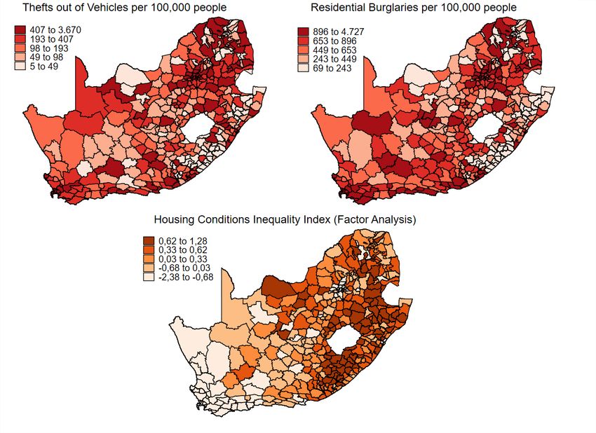
Impressum:

CESifo Working Papers
ISSN 2364-1428 (electronic version)
Publisher and distributor: Munich Society for the Promotion of Economic Research - CESifo
GmbH
The international platform of Ludwigs-Maximilians University’s Center for Economic Studies
and the ifo Institute
Poschingerstr. 5, 81679 Munich, Germany
Telephone +49 (0)89 2180-2740, Telefax +49 (0)89 2180-17845, email office@cesifo.de
Editor: Clemens Fuest
https://www.cesifo.org/en/wp
An electronic version of the paper may be downloaded
· from the SSRN website:       www.SSRN.com
· from the RePEc website:      www.RePEc.org
· from the CESifo website:     https://www.cesifo.org/en/wp
CESifo Working Paper No. 8914

         Crime, Inequality and Subsidized Housing:
                Evidence from South Africa

                                            Abstract

We study the relationship between housing inequality and crime in South Africa. We create a
novel panel dataset combining information on crimes at the police station level with census data.
We find that housing inequality explains a significant share of the variation in both property and
violent crimes, net of spillover effects, time and district fixed effects. An increase of one standard
deviation in housing inequality explains between 9 and 13 percent of crime increases.
Additionally, we show that a prominent post-apartheid housing program for low-income South
Africans led to a reduction in inequality and a decline in violent crimes. Together, these findings
suggest the important role that equality in housing conditions can play in the reduction of crime
in an emerging economy context.
JEL Codes: D630, O100, K140.
Keywords: inequality, crime, economic development.

                Roxana Manea                                        Patrizio Piraino
             The Graduate Institute                            University of Notre Dame
              Geneva / Switzerland                            USA - Notre Dame, IN 46556
       roxana.manea@graduateinstitute.ch                           ppiraino@nd.edu

                                        Martina Viarengo
                                      The Graduate Institute
                                       Geneve / Switzerland
                              martina.viarengo@graduateinstitute.ch

February 2021
We are grateful to the South African Police Service, the Western Cape Department of
Environmental Affairs and Development Planning and Simon Franklin for providing us with data
access. We also thank Tim Swanson for helpful comments and suggestions on an earlier draft. All
remaining errors are our own. Viarengo and Manea gratefully acknowledge the financial support
received from the Swiss National Science Foundation (Research Grant n. 100018-176454 -
Principal Investigator: Dr. Martina Viarengo).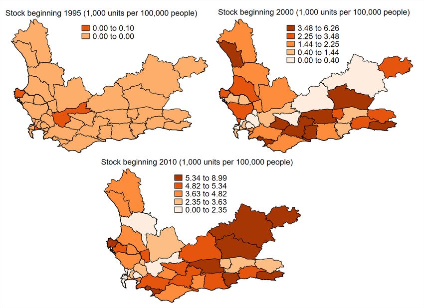
1    Introduction
South Africa is the most unequal country in the world. It has the highest Gini coefficient
in global cross-country comparisons (World Bank, 2020). Besides high inequality, South
Africa also exhibits exceedingly high crime rates. According to the most recent world-
wide homicide ranking, South Africa has a homicide rate which is 6 times larger than
the world average (Global Burden of Disease Collaborative Network, 2018; South African
Police Service, 2020).

Consequently, South Africa provides a unique context to analyze the role of socio-economic
inequalities and their impact on crime. To date, the vast majority of studies on inequality
and crime have focused on income inequality (Kelly, 2000; Enamorado et al., 2016; Kang,
2016; Metz and Burdina, 2018) while a few of them have also looked into consumption-
based or land inequality (Demombynes and Özler, 2005; Buonanno and Vargas, 2019).
Nevertheless, it has become increasingly apparent that economic inequality is just one
dimension of a broader phenomenon. Specifically, housing inequality is particularly im-
portant for countries where a significant percentage of households do not enjoy formal
living arrangements. In post-apartheid South Africa, only 65 percent of households lived
in a formal dwelling (Statistics South Africa, 2012).

In this paper, we aim to provide the first study of the relationship between inequality in
housing conditions and various types of violent and property crimes. We also examine
the role of a major post-apartheid housing program that was introduced by the South
African Government to reduce inequality in living conditions. We evaluate the effect
of this large-scale housing program on inequality and crime in one large province, the
Western Cape. According to our estimates—based on primary data from the Department
of Environmental Affairs and Development Planning (2014) and Franklin (2020)—the
mean stock of housing projects in the Western Cape Province has evolved from 0 to
roughly 2.08 and 4.22 thousand housing units per 100,000 people at the beginning of
1995, 2000 and 2010, respectively. This amounts to approximately 54,250 and 178,500
housing units delivered at the beginning of the years 2000 and 2010, respectively. The scale

                                             2
of this government housing scheme is remarkable—compared to other African countries
and emerging economies in general.1
We draw upon a unique panel dataset. We merge data on crime at the police station level
with socio-economic data from the South African census to form a spatial panel. We collect
information from the universe of police stations in the country on both violent offences
(aggravated assaults, murders and rapes) and property crimes (thefts out of vehicles and
residential burglaries), and we use census data to construct an index describing housing
conditions across South Africa’s former magisterial districts. In addition, we exploit the
spatial nature of the data to identify the magnitude of spillover effects across districts.
Finally, we also merge data on the location of housing projects that were approved by the
Department of Human Settlements in the Western Cape Province. We use this data to
investigate the impact that improved access to adequate housing has had on crime.
We find that housing inequality is positively related to the prevalence of all types of
crime we investigate, except for murders. For most crimes, an increase of one standard
deviation in housing inequality can explain between 9 and 13 percent of increases in
criminal offences. The inequality-crime association is stronger for thefts out of vehicles,
where a standard deviation increase in housing inequality explains 41 percent of the
variation in the number of theft incidents per 100,000 individuals. Spillover effects between
districts are significant and stand at approximately 30 percent of a district’s own crime
levels. Moreover, we show that an increase of 1,000 housing units per 100,000 people
(approximately 0.45 standard deviations) reduces housing inequality by roughly 0.04–
0.16 standard deviations. In terms of impacts on crime, we find that an increase of 1,000
housing units per 100,000 people triggers a 5 to 6 percent reduction in the rate of violent
crimes. To our knowledge, this is the first study that provides evidence of a negative
effect of inequality in housing conditions on crime. This finding is consistent with the
1
According to the Department of Human Settlements, 3 million houses had been delivered by the
end of 2017 in South Africa. On the continent, Algeria comes close, but the context is vastly different
as the State provides most of the Algerian housing (Centre for Affordable Housing Finance in Africa,
2019). Another prominent housing intervention is the Integrated Housing Development Program (IHDP)
in Ethiopia, but its scale pales compared to South Africa (The Economist, 2017). Morocco has also
embarked on a mission to eliminate informal housing arrangements under the Villes Sans Bidonvilles
Program, which started in 2004 and delivered 277,583 housing units—according to the Government of
Morocco (www.mhpv.gov.ma, accessed September 6, 2020). If anything, the provision of government
housing in South Africa is comparable to post-war reconstruction programs in Europe. For instance,
Britain built approx. 3 million units of social housing in 1950–70 (The Economist, 2020).
3predictions of strain theory in criminology. Significant strain can be associated with
inequality in housing conditions because of people’s failure to achieve the fundamental
life goal of decent housing. Agnew (2001) argues that strains that are most likely to cause
an offending behavior are usually high in magnitude, i.e., they are intense or lengthy
and important to the individual, they are perceived as unjust and happen against the
background of low social control.
Our study makes three main contributions to the literature. First, we provide evidence
on the role of a neglected dimension of inequality, housing inequality, and its relationship
with crime. Second, our analysis relies on a panel dataset whereas much of the previous
literature on crime and inequality (particularly in South Africa) has been limited to cross-
sectional analyses. This allows us to account for both the spatial autocorrelation in crime
and for time-invariant unobservables across districts. More generally, we rely on a high-
quality dataset which is very rare in a developing country context. Third, we show that a
large-scale housing program, which reduces housing inequality, also demonstrates promise
in the mitigation of violent crime. Even at the level of high-income economies with higher-
quality data availability, there is insufficient evidence related to housing interventions
(Collinson et al., 2015). For developing countries, the evidence is even scarcer.
The rest of the paper proceeds as follows. Section 2 provides an overview of the literature
while Section 3 presents background information on our context. Section 4 describes
the data and presents descriptive statistics. Sections 5 and 6 present the results of the
empirical analysis. Section 7 provides concluding remarks.
2 Literature
2.1 Inequality, Property and Violent Crimes
Theory
Becker (1968) first introduced the idea of crime as a rational individual choice, whereby
potential offenders compare costs and benefits of criminal acts to decide whether to un-
dertake illegal activities. Consequently, governments can intervene to either reduce the
4attractiveness of criminal participation relative to legitimate living or increase the costs
of crime by making detection easier or punishment harsher.
Building on this insight, some economists have examined the relationship between inequal-
ity and property crimes. For instance, Chiu and Madden (1998) build on Becker (1968)
and suggest that an increase in average income, which happens against the background
of higher inequality, will increase the potential proceeds from illegal activities as well as
the appeal of property-related crimes. This framework also implies that property offences
will disproportionately happen in the relatively richer neighborhoods unless the adoption
of defense technologies becomes widespread. Similar theoretical insights have been put
forward by Freeman (1999), Wu and Wu (2012) and Costantini et al. (2018). Due to its
underlying cost-benefit framework, the economics approach is arguably better suited to
explaining property crimes rather than violent offences (Kelly, 2000; Wu and Wu, 2012;
Draca and Machin, 2015). Property crimes are typically carried out for material gain,
which makes them more amenable to a Becker-type cost-benefit analysis (Kelly, 2000;
Demombynes and Özler, 2005).
The literature in criminology provides additional insights. While inequality is regarded as
a deciding factor in assessing the magnitude of illegal benefits in a cost-benefit framework,
the same phenomenon can also be interpreted as a source of strain leading to anger and
impulsiveness, which in turn makes violent crimes more likely. Strain theory hypothe-
sizes that criminal behavior may be the result of strain that individuals or societies feel.
Such strain is generated by individuals’ failure to achieve positively valued goals (Agnew,
1992,9, 2001). The strains most likely to cause offending behavior are generally high in
magnitude, intense or lengthy and important to individuals, and they are perceived as
unjust (Agnew, 2001). Negative emotions, such as anger, frustration and despair, are the
hypothesized channels that connect strain to crime (Agnew, 1992,9, 2001; Brezina, 2017).
Among these, anger is central to using strain theory to explain violent crimes (Aseltine
et al., 2000; Piquero and Sealock, 2000; Mazerolle et al., 2003).
Empirics
The economic theory of crime is supported by evidence relating to the factors that speak
to the attractiveness (or lack) of legal earning opportunities. Several studies show that
5education is a crime-limiting factor (Lochner and Moretti, 2004; Machin et al., 2011;
Chalfin and Raphael, 2011; Anderson, 2014; Hjalmarsson et al., 2015; Bell et al., 2016).
Other researchers have investigated low wages and unemployment as inducements to a
life of crime (Raphael and Winter-Ebmer, 2001; Gould et al., 2002; Machin and Meghir,
2004; Fougère et al., 2009; Bell et al., 2018; Khanna et al., 2019; Hémet, 2020). A number
of studies also estimate the effects of inequality on crime incidence. In South Africa,
Demombynes and Özler (2005) find a positive and strong correlation between inequality
and property crimes using cross-sectional data. The authors show that the incidence
of property offences is higher in police precincts that are relatively wealthier than their
immediate neighbors. Metz and Burdina (2018) document similar results for a sample
of urban centers in the United States. Bourguignon et al. (2003) further argue that
the leftmost part of the income distribution disproportionately affects property crimes in
Colombia. Thus, a change in income among individuals above a certain threshold would
have no significant effect on mitigating crime. The same type of insight is also posited by
Machin and Meghir (2004).2
The empirical evidence on strain theory comes exclusively from criminology. Using differ-
ent types of data (e.g. macro-level, individual-level, school or neighborhood-level) these
studies find suggestive evidence that strain leads to violence and criminal behavior (Re-
bellon et al., 2009; Mahler et al., 2017; Brezina et al., 2001; Hoffmann and Ireland, 2004;
de Beeck et al., 2012; Warner and Fowler, 2003; Hoffmann, 2003). Although economists
have not explicitly tested strain theory, it has been invoked to explain the relationship
between inequality and violent offences —e.g. Kelly (2000) for metropolitan areas in the
United States; Enamorado et al. (2016) in Mexico, and Buonanno and Vargas (2019)
for Colombia. Kang (2016) further argues that it is a specific type of inequality, i.e.,
segregation and poverty concentration, that drives violent crimes in the United States.
2
Researchers have also sought evidence related to the effectiveness of deterrents such as the size and
intensity of police activities (Levitt, 2002; Di Tella and Schargrodsky, 2004; Evans and Owens, 2007; Lin,
2009; Draca et al., 2011; DeAngelo and Hansen, 2014; Chalfin and McCrary, 2018) or the magnitude
and swiftness of sanctions (Liedka et al., 2006; Drago et al., 2009; Hawken and Kleiman, 2009; Johnson
and Raphael, 2012). Overall, improvements in law enforcement systems are systematically linked to
reductions in crime; however, sanctions appear to be a relatively weak deterrent.
62.2 Crime, Housing Inequality and Related Interventions
The existing literature on the relationship between crime and inequality typically uses
data on consumption, expenditure, land ownership or income. To our knowledge, there
are no studies that investigate the impacts of housing inequality on crime.
A related but distinct stream of literature has evaluated the impacts of programs tar-
geting housing inequality—e.g. giving ownership titles to informal dwellers, providing
infrastructure equitably or introducing housing subsidies. Field (2004; 2005; 2007) find
that an urban titling initiative in Peru significantly increased household labor supply and
household investments and renovations, and reduced fertility. Galiani and Schargrodsky
(2010) document similar evidence for Buenos Aires, Argentina. In contrast, some studies
show no impact or even negative effects of housing subsidies or rent vouchers on individ-
ual outcomes such as labor force participation, earnings and health in the United States
(Susin, 2005; Newman et al., 2009; Jacob and Ludwig, 2012; Jacob et al., 2015) as well
as in India (Barnhardt et al., 2017).
A smaller number of studies (largely on industrialized countries) investigate the effects of
housing programs on crime. For example, Santiago et al. (2003) study public housing in
Denver, Colorado, and argue that the program did not impact neither property or violent
offences. In contrast, Freedman and Owens (2011) and Woo and Joh (2015) find that
the Low-Income Housing Tax Credit program reduced crime in the United States, and in
Austin, Texas, respectively. Freedman and Owens (2011) further argue that the program
has mitigated violent crimes, but it has had no effects on property crimes. Finally, Disney
et al. (2020) show that both violent and property offences have decreased as a result of
the Right to Buy scheme in the United Kingdom, which enabled the tenants of public
housing to buy their dwellings at subsidized prices.
2.3 Crime, Inequality and Housing Policies in South Africa
Although no study has examined the effects of government housing on crime in South
Africa, several papers investigated various determinants of crime. Demombynes and
Özler (2005) study consumption-based inequality and crime using the 1996 census cross-
sectional data. The authors find that inequality is associated with increases in both
7property and violent crimes, although the evidence is stronger for property offences. Sim-
ilarly, Bhorat et al. (2017) study income-based inequality using a cross-sectional dataset
(2011 census) and find a positive link between inequality and property crimes. Other
studies have examined correlates of crime, such as education (Jonck et al., 2015), changes
in ethnic composition around the time of democratization (Amodio and Chiovelli, 2018),
the weather (Bruederle et al., 2017) and social capital in the former apartheid-time reset-
tlement camps (Abel, 2019a).
No study has examined the impact of subsidized housing on crime in South Africa.
Franklin (2020) relies on government housing data for metropolitan Cape Town to show
that low-cost housing developments had a significant and positive effect on household
earnings, particularly those of women. Using data on all metropolitan areas and different
identification strategies, Picarelli (2019) and Lall et al. (2012) find no impact of hous-
ing programs on labor force participation, but document an improvement in children’s
education.
3 Background
3.1 Inequality and Crime
Inequality and crime are pressing issues in South Africa. As an example, the country has
the highest Gini index in the world (World Bank, 2020)3 , and an estimated 65 percent
of the pre-tax national income was captured by the top 10 percent of its earners during
the past decade (World Inequality Database, 2020).4 Moreover, the income share of the
top 1 percent has increased from 10 to 21 percent between 1993 and 2014 (Alvaredo
et al., 2018). In terms of crime, the homicide rate in South Africa is significantly above
the global average and can be regarded as a symptom of wider crime-related problems.
The homicide rate is of 36 reported cases per 100,000 individuals (South African Police
Service, 2018) while the global average is of 6.1 homicides per 100,000 people (United
3
Consumption data from 2014–15 is used to compute the Gini index of South Africa in this cross-
country classification. The data can be retrieved from https://databank.worldbank.org. Accessed De-
cember 20, 2020.
4
Only São Tomé and Prı́ncipe has a higher rate of 68.9 percent, which is a significant increase from
an estimated 60 percent in 2015. The data can be retrieved from https://wid.world/data. Accessed
December 20, 2020.
8Nations Office on Drugs and Crime, 2019).5 Murder rates have remained extremely high,
and this reflects the extraordinary level of violence that exists in South Africa.6
Moreover, property-related crimes are also a serious issue.7 In 2018, 1 in every 24 house-
holds on a suburban block was burgled (Statistics South Africa, 2018). Given the sizeable
magnitude of crime, it is not surprising that this threat is reflected in the way South
Africans go about their daily lives. About 32 percent of individuals reported avoiding
open spaces due to fear of crime, 17 percent were keeping their children from playing
in their neighborhoods and 14 percent were fearful of walking in their own town or us-
ing public transportation (Statistics South Africa, 2018). In addition, about 52 percent
of South African households took significant measures to protect their homes (Statistics
South Africa, 2018). Given the high levels of poverty in the country, this also implies
that a large percentage of households allocate part of their limited resources to home
protection.
South Africa has been suffering from widespread crime and high inequality for a long
time. For instance, the concept of separate and unequal resource allocation was embedded
into South Africa’s apartheid legislation on general facilities, education and employment
(Byrnes, 1996). Although apartheid was formally introduced in 1948, the ideology had
been in place long before (Wilkinson, 1998). This has had long-term consequences for the
socio-economic development of South Africa. In 1991, the legislative pillars of apartheid
were repelled: The Land Act of 1913 and 1936, the Group Areas Act of 1950 and the
Population Registration Act of 1950 (Byrnes, 1996). The new democratic government
came to power in 1994. Several reforms followed.
As a result of concerted development efforts and reforms—including several safety-net
programs, public pension schemes, housing subsidies, school feeding programs, the elim-
ination of school fees for the poor and free healthcare for children, the elderly and other
vulnerable groups—the poverty rate fell from 34 percent in 1996 to 19 percent in 2015
5
2017 statistics are used for comparability. 20,277 murders between April 2017 and March 2018 (South
African Police Service, 2018) for an estimated population of 56,52 million.
6
For the 2019–20 financial year, the rate was still at 36 (South African Police Service, 2020).
7
There are some differences across countries with respect to definitions and propensities to report such
incidents that make it more difficult to compare South Africa with other countries.
9(African National Congress, 1994; World Bank, 2018).8 Moreover, the proportion of the
population with access to basic amenities has continued to increase (World Bank, 2018).
In 1994, 62 percent of individuals had access to electricity. In 2015, the percentage in-
creased to 86. Regarding access to improved water and sanitation facilities, the ratios
went up from 83 to 93 percent and from 53 to 66 percent, respectively (World Bank,
2018). Furthermore, South Africa is close to achieving universal primary and secondary
education, which is key to promoting socio-economic mobility. School attendance among
children aged 6 to 18 has increased from 85 percent in 19969 to 96 percent in 2017 (Statis-
tics South Africa, 2019). Despite these improvements in average wellbeing, crime has
remained high, and South Africa continues to be exceedingly unequal (Alvaredo et al.,
2018; World Bank, 2020; World Inequality Database, 2020).
Using 2015 data, the World Bank (2018) shows that most of the richest decile in South
Africa was connected to the electricity grid and had access to an improved water source:
98 and 97 percent, respectively.10 In contrast, about 78 and 54 percent of the poorest
decile enjoyed these amenities. Similarly, roughly 65 percent of the poor had access to
improved sanitation, while the richest decile was nearing universal access (World Bank,
2018). Lastly, only 2–3 percent of the richest decile were living in overcrowded housing.
The rate among the poorest decile was 68 percentage points higher (World Bank, 2018).11
3.2 Housing Policy
Housing policy in South Africa started off as a racialized scheme around the 1920s. The
1918–20 influenza pandemic likely precipitated the writing of policies and the establish-
ment of institutions intent to segregate South Africans based on race (Wilkinson, 1998).
Between the 1930s and the mid-1970s, housing policy in South Africa served the segrega-
tionist agenda of the apartheid government. This agenda ultimately promoted the concept
8
The World Bank uses international poverty lines in this assessment. Namely, US $1.9 at 2011
purchasing power parity exchange rates. Based on locally measured poverty thresholds, i.e., R758 per
month in terms of 2017 prices, the poverty rate was 40 percent in 2015 (World Bank, 2018).
9
According to the 1996 census. Obtained as the division between full- and part-time students on the
one hand, and the 6-to-18 population less the institutionalized and the “unspecified ” category, on the
other.
10
Calculations of the World Bank based on 2014–15 data.
11
The World Bank uses the number of people per bedroom to measure overcrowding. Two persons per
bedroom is the standard applied to determine whether a household is overcrowded.
10of separate development which implied total apartheid (Wilkinson, 1998). Starting with
the mid-1970s, however, pressure started mounting against the apartheid government.
The urbanization of black South Africans was increasingly regarded as inevitable (Good-
lad, 1996). It was no longer feasible to keep black South Africans away from white urban
centers. In this context, due to a long history of injustices, people in townships started to
revolt (Wilkinson, 1998). Consequently, the government began to slowly relax its vision
of total apartheid, and some measures were taken to increase the housing infrastructure
catering to African households. Nevertheless, these efforts lacked ambition. For instance,
they included the provision of minimally serviced sites on which African households could
build a formal structure at their own expense (Goodlad, 1996; Wilkinson, 1998). Some of
these sites were so poorly located that they remained empty (Goodlad, 1996). They were
referred to as “toilets in the veld ” (Tomlinson, 1998).
With the fall of apartheid in 1994, the provision of adequate housing became a prominent
tool to rebuild South Africa. In fact, housing policies became part of the overarching
Reconstruction and Development Program (RDP). The RDP was the master framework
of that time, an integrated and coherent program of socio-economic transformation that
was designed to enable South Africa to overcome the legacies of apartheid and transition
to a racially inclusive democracy. The Ministry in the Office of the President (1995) has
eloquently summarized the program, which prominently aimed at reducing inequality,
among other objectives.
“The [..] RDP is our response to the serious social and economic problems of
South Africa: mass poverty, gross inequality, a stagnant economy and enor-
mous backlogs.”
In the same document, the RDP is set against a context of inequality, poverty and crime.
“Wealthy suburbs with excellent infrastructure exist side by side with run
down townships, squatter camps and city areas. These are characterized by
overcrowding, poverty and unemployment, poor services, inadequate facilities,
collapsing infrastructure and general decay. Crime and desperation have re-
sulted.”
11During the first year of implementation, 1994–95, the budget allocated to the RDP was
of R2.5 billion out of a R148 billion state budget. For 1995–96, the budget was increased
to 5 billion (Ministry in the Office of the President, 1995). Out of the RDP budget, the
government planned an allocation of R1.4 billion and R1.8 billion to housing in 1994–
95 and 1995–96, respectively (Goodlad, 1996; Tomlinson, 1998). The relative size of
the housing allocation speaks to the importance of this component within the wider RDP
strategy.12 The program was also considered a catalyst for the building, steel and furniture
sectors, an employer for local communities and an engine for the economy (Ministry in the
Office of the President, 1995). At the outset, the goal of the RDP was to provide decent,
well-located and affordable housing to all by 2003 (African National Congress, 1994).
Housing for all was reflective of the vision of the African National Congress. To opera-
tionalize this vision, the RDP’s medium-term ambition was to build 1 million houses in
the first 5 years (African National Congress, 1994; Ministry in the Office of the Presi-
dent, 1995). According to the Department of Human Settlements, only 870,629 houses
had been built by the beginning of the year 2000, which meant that roughly 87 percent
of the target was attained. Although the target was objectively missed and demand far
outstripped the housing units on offer, the achievement was nevertheless significant in the
eyes of South Africans and internationally. On December 24, 1999, the New York Times
ran an article titled “Small Houses a Big Step for South African Pride”.13 It underlined
the fact that these “[. . . ] houses are the most tangible symbol of the post-apartheid gov-
ernment’s commitment to redressing this country’s stark inequalities”. The subsidized
housing infrastructure that was available at the end of 1999 housed 3 million low-income
South Africans in one-room houses at the cost of US $2 billion—the equivalent of approx.
R12.3 billion in 1999 (New York Times, 1999). An additional 3 million people remained
on the waiting list. A South African male interviewed by the New York Times said that
three years of house ownership made him “feel like a man”, although his life and that of
his family still faced a myriad of other problems.
12
Other important destinations were health, education and infrastructure. Regarding health, the RDP
allocated R472.8 and R500 million to the Free Health Care Program in 1994–95 and 1995–96, respectively.
To improve education, R100 million were allocated in 1994–95. With the purpose of improving municipal
services and infrastructure, the RDP further allocated R830 million over a two-year period starting 1994.
Local communities also had access to R250 million for urgent needs in 1994–95. Numbers are sourced
from the report of the (Ministry in the Office of the President, 1995).
13
https:/www.nytimes.com/1999/12/24/world/small-houses-a-big-step-for-south-african-pride.html
12The missed five-year target was due to the construction of housing units starting off
slowly. Out of the 1994–95 budget allocation, only R42 million were used in 1994–95.
Further underspending during the financial year 1995–96 led to a budget of R2.2 billion
for 1996–97 (Goodlad, 1996).14 Progressively, the capacity of the government to deliver
did increase. For instance, between 1994 and 2014, 3.7 million houses and serviced sites
were provided at the cost of R125 billion15 (Department of Human Settlements, 2014).
By the end of 2017, an additional 0.4 million housing opportunities had been delivered.
This was the equivalent of a total of 3 million houses and 1.1 million serviced sites.16
The Reconstruction and Development Program has evolved as it encountered difficulties
and had to adapt. It was followed by the Growth, Employment and Redistribution Strat-
egy in 1996, the Accelerated and Shared Growth Initiative for South Africa in 2005, the
New Growth Path in 2010 and the National Development Plan in 2013 (Adelzadeh, 1996;
Gelb, 2006; Naidoo and Maré, 2015). In parallel, the housing dimension of the original
Reconstruction and Development Program has also evolved throughout the years, along
with the institutions it created and the legislation it inspired. References to RDP have
been relatively more persistent in the context of housing policy. Nevertheless, housing
schemes, too, have often changed name, along with their strategy or implementation
design. Further details on these changes are discussed in Section 6.
In 1994, there were 2.6 million formal housing units in South Africa, 1.7 million shacks
on un-serviced sites and 0.6 million shacks on serviced sites. 1.5 million households were
roofless (Goodlad, 1996). A quarter of the population did not have access to piped
water, and over 40 percent did not have electricity or proper sanitation (Goodlad, 1996).
According to the most recent census data, which were collected in 2011, South Africa had
14.4 million households. Of these, 10.6 million lived in adequate housing (74 percent) and
2.5 million lived in an informal dwelling. The remainder lived in traditional structures. To
put these numbers into context and facilitate comparisons, note that there were 9 million
14
R1 was US $0.22 in January 1997. US $1 in 1997 is worth roughly US $1.6 in 2020.
15
Expressed in 2010 prices. R1 was US $0.15 in December 2010. US $1 in 2010 is worth roughly US
$1.19 in 2020. R1 in 2014 was approx. R0.82 in 2010. As a reference, South Africa’s GDP in 2014
was R3,800 billion (R3,115 billion in 2010 prices). Statistics South Africa. Accessed December 11, 2020.
http://www.statssa.gov.za/?p=4184.
16
Department of Human Settlements. Housing Delivery Statistics. Accessed December 11, 2020.
http://www.dhs.gov.za/sites/default/files/u16/HSDG%20to%20Dec%202017.pdf.
13households in South Africa in 1996. Finally, 2018 estimations have put the proportion of
households living in a formal dwelling at 81 percent (Statistics South Africa, 2019).
Substantial progress has been registered since 1994. Nevertheless, average improvements
hide the fact that some of apartheid’s legacies have not been addressed. The RDP has
been criticized because of its supply-side approach to housing development and the perpet-
uation of spatial segregation, as the dwellers of public housing find themselves physically
distant from economic opportunities (Wilkinson, 1998). In return, socio-economic spatial
segregation breeds crime (Kang, 2016). In a more recent iteration of the housing policy,
the government states its committed to “combating crime, promoting social cohesion and
improving quality of life for the poor ” within its broader vision of achieving “sustainable
human settlements and quality housing” (Department of Human Settlements, 2004).
4 Data and Summary Statistics
4.1 Data
We use three sources of data. First, we rely on census data released by Statistics South
Africa. This includes all the currently existing waves, namely 1996, 2001 and 2011. 2011
is the most recently available wave. Second, we obtained crime data for the financial
years of 1996–97, 2001–02 and 2011–12 from the Crime Statistics and Research Unit of
the South African Police Service (SAPS). The police data includes the universe of crimes
that were either reported by the community or recorded as a result of police action.
The dataset includes detailed information about the type of crime, including numerous
types of violent and property crimes. The SAPS dataset has three dimensions: year,
police station and type of crime. In this study, we use references to police districts and
police stations interchangeably to define the lowest level at which SAPS aggregates crime
indicators. Our third source of data includes the GPS coordinates of government housing
projects in the Western Cape Province, their date of registration and their planned or
approved size. This dataset was obtained from the Department of Environmental Affairs
and Development Planning in the Western Cape, and it was initially published in a
technical report (Department of Environmental Affairs and Development Planning, 2014).
14We have created a unique panel based on the station-level crime statistics, the 2011 census
community profiles and the 10-percent census data for 1996 and 2001. To the best of our
knowledge, this is the first time that the police data is used for this type of research.17
We constructed the dataset as follows. We start with the 2011 census which was compiled
at the lowest possible level of aggregation, roughly 85,000 small area layers that contain
the universe of households and individuals with aggregated characteristics. Since we have
the coordinates of the centroids of these small area layers, we assign them to the polygons
of the administrative units that stand as the common denominator between the 1996 and
2001 waves. South Africa’s 354 former Magisterial Districts (MDs) fulfil this role. MD-
level aggregation thus allows us to append the 1996, 2001 and 2011 census years into a
panel of MD-year observations.18
Then, we merge the census panel with the SAPS panel. SAPS data was provided at the
level of police stations. There are roughly 1,130 police stations, with their number chang-
ing only slightly over time. Some police districts have an irregular shape whose centroid
can easily fall outside district boundaries. This problem can be solved by generating a
random point within the boundaries of police districts instead of using the centroid for
merger. In 35 percent of cases, a police station shares substantial surface with more than
one magisterial district. In order to address this issue, we adopt the following procedure.
We generate multiple random points per police station to better distribute the incidence
of crime between the magisterial districts feeding the crime statistics of the police station
in question. For stations that cross the borders of multiple MDs, we count the points that
fall in each district and assign crimes proportionally to each concerned MD.19 Lastly, we
merge the housing information point-to-polygon with the MD-year spatial panel, where
the points are the project GPS coordinates and the polygons are the MDs.
17
The SAPS data has been used in the literature in cross-sectional analyses, e.g., Demombynes and
Özler (2005) and Bhorat et al. (2017).
18
While the use of weights for the 2011 data was not necessary because the database includes the
universe of households and individuals, we do use weight variables to compute our indicators of interest
at the level of MDs in 1996 and 2001.
19
This assumes that crimes are homogeneously distributed within the boundaries of any police station.
We believe this assumption is unlikely to have significant consequences as the size of police districts is
proportional to the size of their population and cities have several police districts. If cities were part of
larger police districts, crimes would be concentrated in and around the city, while the outside territory
would be less afflicted. Police stations with large territories are usually sparsely populated. See Appendix
A.4 for a presentation of the merger between MDs and stations.
15The result is a panel of 354 MDs observed 3 times, in 1996, 2001 and 2011. This rep-
resents a total of 1,062 observations. Census data is representative at the level of MDs,
and we use this data to compute inequality indices and average socio-economic charac-
teristics. Each MD is populated with crime data, which is sourced from the universe of
crime incidents reported to police stations across the country. Regarding the government
housing data, the sample is limited to the universe of housing projects in the Western
Cape Province. The Western Cape sample has 42 MDs observed 3 times, which amounts
to 126 observations.
This dataset is the first to allow the analysis of South African census and police infor-
mation in a panel setup. It is also the first dataset to include project information on
government housing for the Western Cape Province. Franklin (2020) also uses project-
level data, but his focus is limited to metropolitan Cape Town. Finally, this is a spatial
panel, which allows us to grasp the magnitude of crime spillover effects between adminis-
trative units and model the spatial interdependence of MD-level unobservables.
4.2 Measurement of Crime and Inequality
The data we use consists of crimes reported to the police. As acknowledged in the litera-
ture, objective measures of crime have several advantages with respect to the self-reported
victimization rates. On the other hand, failing to include incidents that are not reported
to the police is considered less consequential (Pudney et al., 2000; Rufrancos et al., 2013).
We measure crime as the natural logarithm of crime incidence per 100,000 people to
normalize the distribution of the variable.
In order to construct the housing inequality index, we rely on six variables that are indica-
tive of the quality of the housing infrastructure: type of dwelling (permanent, traditional
or informal), access to water (tap water inside the building, in the yard, on a commu-
nity stand or no access to piped water), type of toilet facilities (flush/chemical toilet, pit
latrine, bucket latrine or no toilet facilities), type of fuel for cooking and heating (electric-
ity/solar/gas, paraffin/coal or wood/animal dung), and type of fuel for lighting (electric-
ity/solar, paraffin/gas or candles). These are the defining aspects of adequate housing.20
20
Regarding the measurement of housing inequality in the general literature, some researchers rely
on variables such as surface size, number of rooms or selling value to measure housing inequality (Tan
16These are also the housing dimensions that the intervention we evaluate, the subsidized
housing program, has targeted in terms of outcomes—whether directly (dwelling type,
access to water, type of toilet facilities and electricity) or indirectly (type fuel for cooking
and heating via the availability of electricity and the ability to safely store and accumulate
assets). We start by computing inequality in terms of each of these six variables. Then,
based on the standardized values of the inequality measures, we use factor analysis to
reduce the number of variables and summarize their information into one index, i.e., the
latent variable that describes inequality in terms of housing conditions. Appendix A.1
shows the factor analysis. There is only one factor with an eigenvalue greater than 1, and
the Kaiser-Meyer-Olkin measure of sampling adequacy stands at 0.83. To demonstrate
the robustness of our results, we show in the appendix that our findings hold for other
combinations of the variables that serve the computation of the inequality index.
K
X i
X
Inequality = − pi × ln pj (1)
i=1 j=1
To accommodate the fact that the variables describing housing conditions are sets of
ordered categories, we rely on Cowell and Flachaire (2017) to compute inequality. See
Equation 1, where K stands for the number of categories, which are ordered starting from
the best one and moving down to the worst. That is, j = 1 corresponds to houses made
from permanent materials, the availability of tap water inside the household’s dwelling,
the availability of flush or chemical toilets, and the use of electricity or solar energy for
lighting, cooking and heating purposes. The larger the number of people who move into
the top category, the greater will be the decline in inequality. pi is the probability of an
individual belonging to category j = i.
et al., 2016; Tunstall, 2015). Others take a multidimensional approach to quantifying access to adequate
housing, which is sometimes confounded with an asset index. These studies use variables that describe
the quality of wall, floor or roof materials, the presence of basic amenities, asset ownership, access to
roads, schools, hospitals, etc. (Filmer and Pritchett, 2001; McKenzie, 2005; Van Phan and O’Brien,
2019).
174.3 Summary Statistics
Table 1 reports the summary statistics that describe the 1,062 MD-year observations in
the analytical sample.21 Table 1 shows that crime incidence has increased slightly between
1996 and 2001, and it has thereafter decreased sharply. Murders have been the exception.
They have decreased across all waves. The inequality index points to a gentle decrease
between 1996 and 2001, and a sharp decrease between 2001 and 2011. The percentage
of unemployed and discouraged individuals has followed the same pattern. Moreover,
average education has improved significantly between 1996 and 2011, and so have most
variables proxying for household socio-economic status. Lastly, there is also an indication
of post-apartheid rearrangements of the population, as the percentage of people on the
move was particularly large in 1996 and 2001.
[Table 1: Descriptive Statistics. Insert here.]
Figures 1a and 1b present the raw crime categories that are reported by the South African
Police Service for violent and property crimes, respectively.22 These figures include the
analytical sample, 1996, 2001 and 2011, and the out-of-sample year of 2019 to give an
indication of the current situation. Figures 1a and 1b confirm the insights of Table
1, i.e., crime incidence has first increased between 1996 and 2001 and then decreased.
Exceptions do exist. For instance, the incidence of rapes and thefts out of vehicles has
generally decreased between 1996 and 2019, although the decrease between 1996 and 2001
was less pronounced. Moreover, murders have decreased between 1996 and 2011, but then
exhibited an uptick in 2019.
[Figure 1a: Violent Crimes. Insert here.]
[Figure 1b: Property Crimes. Insert here.]
Figures 1a and 1b also motivate our choice of dependent variables. First, we see that
aggravated assaults are the most commonly reported type of violent crime. Moreover, as
21
In computing these summary statistics, MDs are assigned the same weight regardless of their popu-
lation or surface.
22
Figure 1a would have been the universe of violent crimes; however, due to the imperfect overlap
between crime categories across the years, we had to drop some sexual offences. As far as reporting to
the police is regarded, the magnitude of these sexual offences is small. Therefore, their omission does not
impact the message of Figure 1a. Figure 1b presents the universe of property crimes.
18the literature shows that murders are less likely to suffer from misreporting, we decided
to include them in our analysis. Furthermore, we also explore the evolution of rapes
because crimes against women have been at the forefront of debates in South Africa.
Additionally, we also focus on the two most reported types of property offences, which
consist of burglaries at residential places and thefts out of vehicles. These are also the
crime categories that are most often analyzed in the literature (Kelly, 2000; Lochner and
Moretti, 2004; Demombynes and Özler, 2005; Kang, 2016).
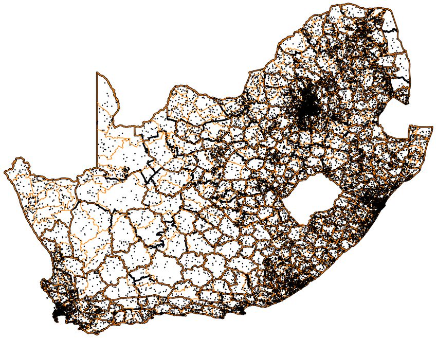
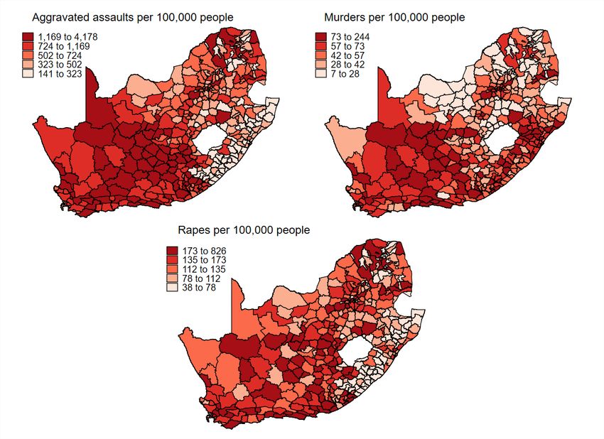
[Figure 2: Spatial Distribution of Variables. Insert here.]
Finally, Figure 2 shows the spatial distribution of crime and housing inequality across
South Africa’s MDs and averaged over the three waves of data. We see that violent crimes
cluster in the Western, Northern and Eastern Cape Provinces, while property crimes
are predominant in and around metropolitan areas. Finally, inequality shows a spatial
pattern whereby higher values cluster in the Eastern half of the country, particularly in
and around the areas which were designated by the apartheid regime for occupation by
black populations to serve segregationist agendas.
The summary statistics presented in this section suggest a positive relationship between
crime and housing inequality. Inequality has only slightly improved between 1996 and
2001, while it has registered a substantial decrease between 2001 and 2011. In parallel,
crime has followed a similar path. Between 1996 and 2001, progress was minimal. Some
types of crime have even registered an increase in their incidence. Starting from 2001,
however, crime incidence has declined. These trends are supportive of our hypothesis, per
which improvements in inequality may help reduce the incidence of crime. We explore
this link in the following sections by conducting a spatial fixed effects analysis. Moreover,
we evaluate the impact of a large-scale housing program on inequality and crime.
5 Empirical Analysis
5.1 Housing Inequality and Crime
In order to estimate the relationship between housing inequality and crime, we take ad-
vantage of variation over time and across space by using a balanced panel of magisterial
19districts. We begin our estimations with a fixed effects model as presented in Equation 2:
Cnt = αn + λt ιn + βHnt + Xnt γ + nt (2)
Cnt = (C1t , C2t , . . . , CN t )T is the natural log of crime incidence per 100,000 people, where
n represents the magisterial district and t represents the time period. As discussed above,
we have N = 354 magisterial districts and T = 3 waves of data, 1996, 2001 and 2011.
Hnt is the housing inequality index. Equation 2 includes both the district fixed effects α
and the time fixed effect λ.23 Xnt includes covariates such as time-varying individual and
household characteristics (averaged at the magisterial district level) as well as population
density, as presented in Table 1.
[Table 2: Fixed Effects Estimates. Insert here.]
Table 2 shows the coefficient estimates deriving from the fixed effects model. We estimate
the model separately for different types of violent and property crimes. The results show
a positive association between housing inequality and crime rates. This is true for all
types of crimes, with the exception of murders and residential burglaries, where we do
not find a statistically significant coefficient. Controlling for a large set of confounding
factors, Table 2 shows that a standard deviation increase in the housing inequality index
is associated with an approximate increase of 0.108 and 0.085 log points, i.e., 11 and 9
percent, in overall violent and property crimes, respectively. When looking at specific
types of crimes, we notice that thefts out of vehicles appear to be particularly sensitive
to housing inequality, as the coefficient reaches 0.449 log points. Table 2 also reports the
coefficient estimates for some of the control variables included in the model. In particular,
we note a generally negative correlation between average education and crime.
As a robustness check, we also use a non-linear specification to account for the fact that
the distribution of the untransformed crime variables resembles a Poisson. The estimated
coefficients are reported in Appendix A.3. The coefficients on housing inequality are very
similar in the two specifications.
23
τ is a vector of 1s.
205.2 Accounting for Spillover Effects
The estimation above does not take into account the potential spillover effects across
magisterial districts. In order to measure spillover effects, we can use a spatial model.
This amounts to including a spatial lag on the dependent variable as follows:
Cnt = αn + λt ιn + ρWn Cnt + βHnt + Xnt γ + ηnt (3)
where ηnt = φMn ηnt + εnt , and W and M are square matrices that describe the spatial
dependency between magisterial districts. W applies the same positive weight for con-
tiguous spatial units and a zero weight for all other units, while M is the inverse distance
weighting matrix. ρ and φ are scalars.24
The specification above implies that any change to an explanatory variable in a given
magisterial district can affect the dependent variable in that district’s neighbors via in-
creases in own crime, which spills into other districts provided that ρ is different from
zero. This allows us to estimate a spatial autoregressive combined (SAC) model with
individual and time fixed effects, as presented in Equation 4 (LeSage and Pace, 2009; Lee
and Yu, 2010).
Cnt = (In − ρWn )−1 (αn + λt ιn + βHnt + Xnt γ) + (In − ρWn )−1 (In − φMn )−1 εnt (4)
The defining characteristics of a SAC model are the inclusion of a spatial lag on the
dependent variable and the spatial interdependence of the disturbance terms. The SAC
specification controls not only for time-invariant omitted variables, but also controls (at
least partially) for time-varying omitted variables or unobserved latent influences that
explain the spatial clustering of the dependent variable (LeSage and Pace, 2009). It is
well established that crime incidence exhibits spatial dependency, e.g., crime hotspots
24
We maintain that individuals are unlikely to travel across multiple districts to perpetrate crimes.
Thus, the W matrix is appropriate. However, we are less restrictive about the spatially correlated
unobservables, which we assume can be similar beyond first-order neighbor, hence the M matrix. If
the scalars are not statistically different from zero, then the use of spatial lags is not necessary for the
dependent variable or the error term, respectively.
21(Chainey et al., 2008; Ratcliffe, 2010). The use of spatial models is in fact relatively
common in studies of crime as they help mitigate the omitted variables bias.
It is important to note that the spatial dependency of the district observations makes
the estimated coefficients of interest not as easily interpretable, as the derivative of the
dependent variable with respect to the explanatory variables is no longer simply β or γ.25
Instead, average direct and total effects can be computed (LeSage and Pace, 2009).
For a given magisterial district n, the average direct impact measures the effect of a change
in Xn on crime in district n inclusive of feedback loops, whereby observation n affects
its neighbor, and these neighbor will, in return, loop back and affect n.26 The average
total impact for district n includes the own derivative (direct impact) and all of the cross
derivatives (the indirect impact or spillover effects) (LeSage and Pace, 2009).
While spillover effects motivate the inclusion of spatial lags in the dependent variable, the
spatial lags on the error term are motivated by the assumption of spatial heterogeneity
(LeSage and Pace, 2009). Thus, in addition to the individual heterogeneity modelled by
the fixed effects framework, we are now allowing some of the unobserved characteristics
of any given district to be similar to those of its neighbors. The intensity of this similarity
is decreasing the further away districts are from each other. Importantly, we assume that
these unobserved characteristics are unrelated to the observed covariates.27
[Table 3: Spatial Autoregressive Combined, Fixed Effects Estimates. Insert here.]
Table 3 shows the results from estimating Equation 4. Spillover effects, as estimated by ρ,
appear to be present in all cases. In most cases, spillover effects from neighboring districts
are roughly one third of a district’s own crime incidence. φ is also generally significant,
which points to the existence of spatial heterogeneity in the error terms. If the SAC model
identifies the data generating process correctly, then the estimates in Table 3 will suffer
less from omitted variables compared to the simple fixed effects model. This allows us to
25 k
This is because the derivative of Cnt with respect to Xmt , where m can be different from n, is
potentially non-zero. k denotes the kth variable in the X matrix.
26
District n will thus suffer from the crime it fuels in neighbouring districts due to an increase in own
crime incidence.
27
We also assume that spillover effects at the borders between South Africa and its neighbouring
countries are negligible. Since these are national borders, with strict controls, it seems a plausible
assumption.
22get as close as possible (given the available data) to a causal interpretation of the effects
of housing inequality on crime rates.
For violent crimes, the estimated direct effect of housing inequality is 0.085 log points
(8.9 percent), while the total effect, which accounts for spillover effects from neighboring
districts, is about 0.109 log points. The direct impact of housing inequality on aggravated
assaults and rape is 0.094 and 0.124 log points, respectively. In the same order, the total
impacts are 0.124 and 0.135 log points. Lastly, the coefficient on education is negative
across the board—districts that are more educated have less crime. The direct impact of
a one-year increase in average education varies between a reduction of 0.130 log points in
the case of rapes and 0.204 for murders.
Moving to property crimes, we note that spillover effects are slightly smaller than those for
violent crimes, although there is one notable exception: thefts out of vehicles. Moreover,
compared to the fixed effects estimates, the spatial estimates display a more consistent
pattern across types of property crime. The impact of housing inequality on residential
burglaries is positive and significant. The direct and total effects are 0.086 and 0.105 log
points, respectively. Similarly, the direct impact of an increase of one standard deviation
in housing inequality triggers a 0.099 log points increase in all property crimes—the
equivalent of 10.4 percent. In the case of thefts out of vehicles, the direct impact is 0.345
log points, i.e., 41 percent. The total impacts are 0.124 and 0.522 log points, respectively.28
Education is also negatively related to property crimes across the board. Appendix A.3
shows that the results in Table 3 are robust to the choice of variables that are used to
build the housing inequality index as well as to the use of a principal component analysis
instead of factor analysis.29
In summary, the empirical results in this section show that higher inequality in terms of
housing conditions is associated with higher crime, whether violent or property related.
While these are not estimations of the causal impact of housing inequality on crime, they
do account for spillover effects across space as well as time and magisterial district fixed
28
The relatively higher responsiveness of thefts out of vehicles to inequality may be explained by this
crime’s more opportunistic nature and ease of perpetration.
29
In the order in which the indices are presented in Appendix A.3, the Kaiser-Meyer-Olkin measures of
sampling adequacy are 0.83, 0.83, 0.76 and 0.68. Each analysis recommends only one factor or principal
component. All factor loadings are positive.
23You can also read