Defining priority areas for blue whale conservation and investigating overlap with vessel traffic in Chilean Patagonia, using a fast fitting ...
←
→
Page content transcription
If your browser does not render page correctly, please read the page content below
www.nature.com/scientificreports
OPEN Defining priority areas
for blue whale conservation
and investigating overlap
with vessel traffic in Chilean
Patagonia, using a fast‑fitting
movement model
Luis Bedriñana‑Romano1,2*, Rodrigo Hucke‑Gaete1,2*, Francisco A. Viddi1,2, Devin Johnson3,
Alexandre N. Zerbini3,4,5,6, Juan Morales7, Bruce Mate8 & Daniel M. Palacios8
Defining priority areas and risk evaluation is of utmost relevance for endangered species`
conservation. For the blue whale (Balaenoptera musculus), we aim to assess environmental habitat
selection drivers, priority areas for conservation and overlap with vessel traffic off northern Chilean
Patagonia (NCP). For this, we implemented a single-step continuous-time correlated-random-walk
model which accommodates observational error and movement parameters variation in relation to
oceanographic variables. Spatially explicit predictions of whales’ behavioral responses were combined
with density predictions from previous species distribution models (SDM) and vessel tracking data
to estimate the relative probability of vessels encountering whales and identifying areas where
interaction is likely to occur. These estimations were conducted independently for the aquaculture,
transport, artisanal fishery, and industrial fishery fleets operating in NCP. Blue whale movement
patterns strongly agreed with SDM results, reinforcing our knowledge regarding oceanographic
habitat selection drivers. By combining movement and density modeling approaches we provide a
stronger support for purported priority areas for blue whale conservation and how they overlap with
the main vessel traffic corridor in the NCP. The aquaculture fleet was one order of magnitude larger
than any other fleet, indicating it could play a decisive role in modulating potential negative vessel-
whale interactions within NCP.
Animal movement integrates several scales of ecological phenomena, including individual physiological state,
locomotive, and navigational capabilities, and how these interact with external (environmental) factors affecting
prey distribution. This has been explicitly acknowledged by theoretical approaches that place movement into a
wider ecological and evolutionary framework1–3. Coupled with this growth in movement ecological theory, the
rapid increase in animal tracking technology has allowed researchers to expand the frontiers of the questions
that can be answered4,5. It is not surprising then, that movement approaches are being increasingly used as an
ecological tool for informing conservation and management a ctions6–8. In fulfilling this goal, telemetry data have
become particularly useful for oceanic species with wide-ranging life histories, for which other more traditional
monitoring approaches are logistically challenging9.
1
Instituto de Ciencias Marinas y Limnológicas, Facultad de Ciencias, Universidad Austral de Chile, Casilla 567,
Valdivia, Chile. 2NGO Centro Ballena Azul, Valdivia, Chile. 3Marine Mammal Laboratory, Alaska Fisheries Science
Center/NOAA, 7600 Sand Point Way NE, Seattle, WA, USA. 4Marine Ecology and Telemetry Research, 2468 Camp
McKenzie Tr NW, Seabeck, WA 98380, USA. 5Cascadia Research Collective, 218 ½ 4th Ave, Olympia, WA 98502,
USA. 6Instituto Aqualie, Av. Dr. Paulo Japiassú Coelho, 714, Sala 206, Juiz de Fora, MG 36033‑310, Brazil. 7Grupo
de Ecología Cuantitativa, INIBIOMA‑CONICET, Universidad Nacional del Comahue, Bariloche, Argentina. 8Marine
Mammal Institute and Department of Fisheries and Wildlife, Hatfield Marine Science Center, Oregon State
University, Newport, OR, USA. *email: luis.bedrinana.romano@gmail.com; rhucke@uach.cl
Scientific Reports | (2021) 11:2709 | https://doi.org/10.1038/s41598-021-82220-5 1
Vol.:(0123456789)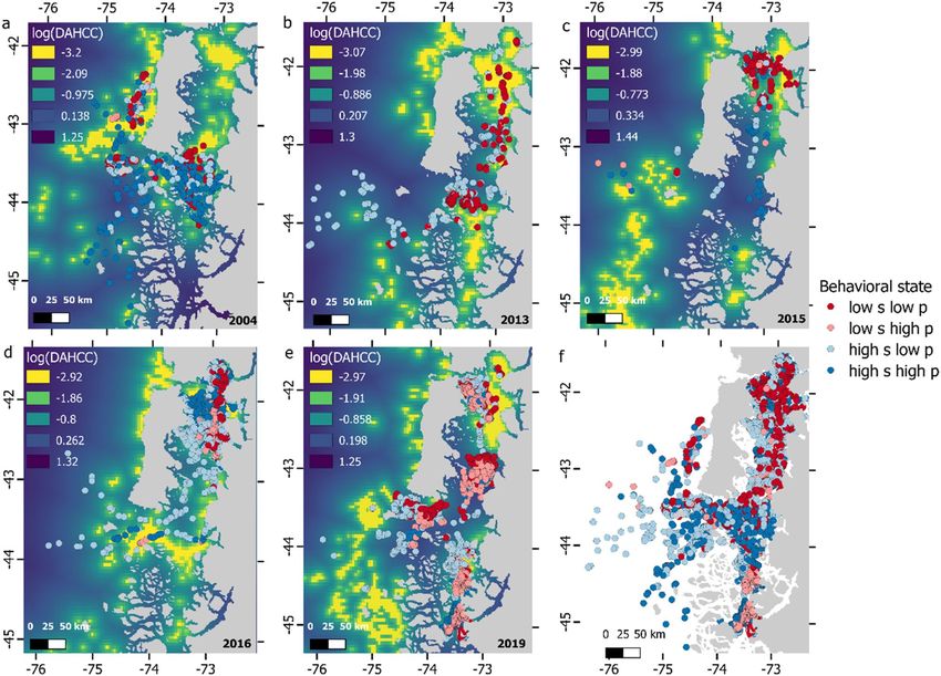
www.nature.com/scientificreports/
For the endangered Eastern South Pacific (ESP) blue whale (Balaenoptera musculus) population, northern
Chilean Patagonia (NCP) is regarded as its most important summer foraging and nursing g round10–12. Previous
studies on blue whale occurrence and movement patterns indicated that until the onset of austral autumn/winter
migration, blue whales focus most of their activities within these productive coastal w aters12–15. However, vari-
ations in how this population utilizes this region and other areas within the ESP appear to result from changes
in prevailing oceanographic c onditions16.
Species distribution models (SDM) have shown that austral spring chlorophyll-a concentration, prior to
the whales’ arrival, and thermal fronts are important oceanographic proxies for describing the abundance and
distribution patterns of blue whales within the N CP16. Krill, the primary prey of blue w hales17, can take advan-
tage of seasonally enhanced productivity for biomass production, with some time lag linking early life-history
stages (e.g. larval recruitment) with adult densities17–21. Adult krill biomass is subsequently concentrated by
thermal fronts into high-density patches which blue whales prey u pon22–25. This prey aggregation effect driven
by thermal fronts could be critical for blue whales, and other large baleen whales, given their energetically costly
feeding behavior26–29. We hypothesize that both time-lagged distribution of primary productivity and thermal
front aggregating effect generates foraging conditions for blue whales within NCP. To further test predictions
from this hypothesis, here we propose that individual blue whales modify their behavior within areas of high
spring chlorophyll-a concentrations and/or thermal front occurrence. As foraging behavior cannot be directly
assessed solely by inspecting tracking data, we consider area-restricted search behavior (ARS, lower velocity and
ehavior30,31.
less directional persistence) as a proxy for this type of b
Potential local threats affecting blue whales in NCP include collisions with vessels due to intense maritime
traffic16,32, negative interactions with aquaculture and fisheries activities33–35, direct and indirect effects from
poorly regulated whale-watching operations36, and general disturbance from noise and acoustic pollution37. As
such, identifying priority areas for focusing conservation actions is of utmost relevance considering a population
numbering the low hundreds with a very low potential biological removal from anthropogenic origin estimated
at 1 individual every 1.8 years16 for continued growth.
Vessel collisions with cetaceans have become recognized worldwide as a significant source of anthropogenic
mortality and serious injuries38–41. Empirical work on this issue has been conducted in a few areas and popula-
tions, mostly in the northern Hemisphere32,39,42,43, with little effort conducted in South America32,44. In most
countries, unreported cases, limited monitoring and insufficiently documented incidents have precluded any
accurate assessment of the true collision prevalence and trend analyses32.
Given the earlier results from SDMs, we considered using telemetry data as a complementary tool for improv-
ing our understanding of blue whale habitat selection process16,17,45 and investigating overlap with vessel traffic
in NCP. In fulfilling these goals, here we provide: i) a novel fast-fitting model application for data gathered from
satellite-monitored Argos tags (hereafter Argos tags), ii) model-derived spatial predictions of how whales use
the area based on prevailing oceanographic conditions during the tracking period, iii) spatial estimates on the
relative probability of encountering blue whales, based on the integration of movement model predictions with
those of a previous SDM, and iv) spatial estimates on the relative probability of whales encountering vessels as
a measure of risk for four different vessel fleets operating in NCP.
Methods
Study area. The NCP (41–47°S) is characterized by an intricate array of inner passages, archipelagos, chan-
nels, and fjords enclosing roughly 12,000 km of convoluted and protected shoreline (Fig. 1). Primary biological
productivity here is modulated by the mixing of sub-Antarctic waters, rich in macro-nutrients, and the abundant
input of freshwater (derived from river discharges, heavy precipitation and glacier/snow melt), rich in micro-
nutrients, particularly silica46–48. Within the NCP, several micro-basins have been described, some of them hav-
ing particularly high seasonal primary and secondary production46–50, providing resources that upper-trophic
level species rely on12,17,50–54. The area also hosts one of the largest salmon aquaculture industries in the world,
among other anthropogenic activities that negatively affects local biodiversity33,34,55.
Tagging and telemetry data. Argos tags were deployed on 15 blue whales during the austral summer
and early autumn at their summering grounds off the NCP (Fig. 1), following procedures described e lsewhere14.
Briefly, whales were tagged in waters of Corcovado Gulf during February 2004 (n = 4), and the Chiloe Inner Sea
during late March and early April 2013 (n = 2), 2015 (n = 3), 2016 (n = 2) and 2019 (n = 4). Tags were deployed
using a custom-modified compressed-air line-thrower (ARTS/RN, Restech N orway56) set at pressures ranging
between 10 and 14 bar. Several models of custom-designed fully implantable satellite tags were used, including:
ST-15 [n = 4], manufactured by Telonics (Mesa, Arizona, USA), SPOT5 [n = 3], SPOT6 [n = 4], and MK10 [n = 4],
manufactured by Wildlife Computers (Redmond, Washington, USA).
Raw Argos data included locations within NCP and outside the area after the onset of migratory movement.
Because we were concerned with understanding movement patterns within the NCP, we applied a cut-off point
of 24 h prior to a clear sign of migration was observed. This subset of the data was filtered using the R package
“argosfilter”57 removing relocations that comprised velocities exceeding 3 m s−1, this upper limit was defined
based on previous maximum speed assessments for this p opulation14.
Oceanographic covariates. Chlorophyll-a and sea surface temperature (SST) data were extracted using R
package “rerddapXtracto”58, which accesses the ERDDAP server at the NOAA/SWFSC Environmental Research
Division. Chlorophyll-a data corresponded to satellite level-3 images from the Moderate Resolution Imaging
Spectroradiometer (MODIS) sensor onboard the Aqua satellite (Dataset ID: erdMH1chlamday), corresponding
to monthly averages in a grid size of 4.64 × 4.64 km. Distance to areas of high chlorophyll-a concentration during
Scientific Reports | (2021) 11:2709 | https://doi.org/10.1038/s41598-021-82220-5 2
Vol:.(1234567890)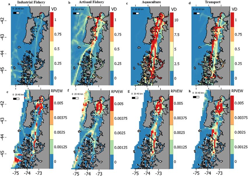
www.nature.com/scientificreports/
Figure 1. Map of the Chilean Northern Patagonia depicting relevant geographical landmarks, tagging locations
and the year of each deployment. Maps were created in R ver. 4.0.2 (https://www.r-project.org) and ensembled
in QGIS ver. 3.8.0 (https://www.qgis.org) for final rendering. Maps were created using data on bedrock
topography from the National Centers for Environmental Information (https://maps.ngdc.noaa.gov/viewers/
grid-extract/index.html). Values above 0 were considered land coverage.
spring (DAHCC), defined as the distance to polygons enclosing areas with an average chlorophyll-a concentra-
tion equal or higher than 5 mg/m3 during austral spring months (September, October, November), was the best
explanatory variable in a SDM applied to line-transect survey data for blue whales in N CP16. Here we used the
same procedure to construct this covariate but used the 95th percentile of each year´s concentrations distribu-
tion within the study area as the cut-off point for defining areas of high chlorophyll-a concentration. This was
preferred because whales might select areas with the highest productivity regardless of their absolute values.
Maps for DAHCC were created for each year where telemetry data were available, and their values were log
transformed to reduce data overdispersion before their use in the models.
For SST, data corresponded to daily averages of level-4 satellite images derived from the Multi-Scale Ultra-
High Resolution (MUR) SST Analysis database (Dataset ID: jplMURSST41). MUR-SST maps merge data from
different satellites, combined with in-situ measurements, using the Multi-Resolution Variational Analysis sta-
tistical interpolation59, in a grid size of 0.01 × 0.01 degrees (ca. 1 km2). From MUR-SST maps, thermal gradients
maps were generated for each day that whale locations were available using the R package “grec” v. 1.3.060 with the
Contextual Median Filter a lgorithm61 as the method for calculating gradients. MUR-SST and thermal gradients
maps were used to extract the associated covariate values for each whale location.
Vessel traffic data. To characterize vessel traffic patterns in the area, daily vessel tracking information
(time-stamped GPS locations for individualized vessels) was obtained from the Chilean National Fisheries and
Aquaculture Service (SERNAPESCA), available at www.sernapesca.cl. This database was released by the Chilean
government during 2020 and comprises data involving the industrial and artisanal fisheries, aquaculture, and
transport fleets, from March 2019 to present (updated daily). According to Chilean legislation it is mandatory for
these fleets to provide tracking information to SERNAPESCA, except for artisanal fishing vessels smaller than
15 m and also for those smaller than 12 m in the case of artisanal purse seiners (www.bcn.cl). Artisanal fishing
fleet comprises vessels up to 18 m in length and less than 80 cubic meters of storage capacity; above these metrics
fishing vessels are considered part of the industrial fishing fleet. The transport fleet comprises vessels with no size
limitations, engaged solely in the transportation of fishery resources. The aquaculture fleet is the most diverse
Scientific Reports | (2021) 11:2709 | https://doi.org/10.1038/s41598-021-82220-5 3
Vol.:(0123456789)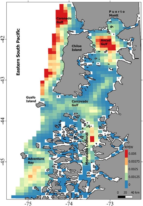
www.nature.com/scientificreports/
one, considering its different operations (e.g. staff commuting, live and processed resource transportation, and
supplies and infrastructure movement) with vessel sizes ranging from 5 to 100 m.
All procedures described next were conducted independently for each fleet during data analyses. We used an
8 × 8 km grid to calculate vessel density (VDi) for each grid-cell i. Vessel data are provided daily, with data gaps
occurring for some days. Therefore, VDi was calculated by summing the daily number of unique vessels cross-
ing each grid-cell i in a month divided by the total number of days with available data (range: 25–31 days). This
procedure was conducted for austral summer and austral autumn months (March-June of 2019 and January-June
of 2020) and then averaged into a single layer. Potential large differences in traffic patterns between these months
were visually inspected through plots, which can be found as Supplementary Figures S1–S4 online. Data from
austral winter and austral spring months were not used as most of the blue whale population is absent from the
study area during these m onths13,14.
Modeling approach. Telemetry data analysis has motivated the development and increasing use of various
state-space modeling (SSM) approaches, which deal with path reconstruction and complex latent behavioral
states30,31,62,63. Most practical applications of SSM, however, are computationally intensive and therefore require a
long time for fitting them. Recently, SSM has been implemented via Template Model Builder (TMB), a R package
that relies on the Laplace approximation combined with automatic differentiation to fast-fit models with latent
variables64–66. Based on “TMB” tools, we fitted a continuous-time correlated-random-walk model (CTCRW)
which estimates two state variables, velocity and true locations from error-prone observed locations, and two
parameters, β controlling autocorrelation in directionality and velocity and σ controlling the overall variability
in velocity62. Variances for modelling error in locations were derived from the Argos error e llipse67. As the error
ellipses data were not available for tags deployed in 2004, we calculated the mean error ellipse for all location
classes in the newer tags (2013–2019) and assigned these values to the corresponding location classes for tags
deployed in 2004.
The original version of this model (with no behavioral variation) was fitted to obtain estimates of the true
locations in whale’s paths and used these to extract the corresponding covariate values from DAHCC, SST and
thermal gradients rasters. The mean of the covariate values within a 3 km radius from each estimated location
was used to partially account for uncertainty in covariate data arising from observation error. This error radius
corresponded to twice the known error for Argos location classes 3, 2 and 167. Covariate data were standard-
ized, and missing values were filled with zeros, which correspond to the mean in standardized variables. This
only affected 6 whales (ID#s 1,6,7,10,11 and 12), it was restricted to SST and thermal gradient data, and except
for one whale never exceeded more than 2.7% of the data (with ID#7 at 10.4% of the data). We modified the
original version of the CTCRW by allowing βtand σtto be random variables that vary in time as a function of
environmental covariates.
log(σ t ) ∼ Normal(µ1,t , ε1 )
µ1,t = A0 + AXt
log(βt ) ∼ Normal(µ2,t , ε2 )
µ2,t = B0 + BXt
where B0 and A0 are intercepts, A and B are vectors of slopes, Xt is the corresponding design matrix holding the
standardized covariates, and ε1 and ε2 correspond to standard deviations. In every case, the estimated standard
deviation ε2 for βt was extremely small and presented exceptionally large standard errors; therefore, instead of
trying to estimate this parameter, we fixed it at 0.01. In cases where no covariate presented a significant effect
on βt this variable was reduced to a single parameter β, which was estimated. Estimated values of β larger than 4
produce persistence values lower than 0.05 h, indicating that at very short time differences velocity and location
are poorly correlated with previous values. Therefore, in cases where model estimates for β were higher than 4
(ID#s 5 and 10) β was fixed at 4 indicating overall poorly autocorrelated movement patterns.
Our modelling approach allowed us to quantify the influence of environmental covariates on βt and σt , with
higher values of σt indicating higher velocities and higher values of βt indicating lower directional persistence,
which might be expressed as pt = 3/βt in units of t ime62. As no discrete behavioral states were explicitly included
in our model, we defined behavioral states as post hoc categories based on pt and σtvalues and their medians.
The expected ARS state (slower and less persistent movement) was defined for locations jointly holding values
of pt and σtbelow their medians and the opposite was defined as transit state. The other two logical combinations
(high pt with low σt and low
√ pt with high σt) were also provided and their interpretation is further discussed below.
We also calculated νt = √πβ ∗σ t
, which corresponds to long-term velocity68. This variable is a function of both
t ∗2
σtand βt(or pt), and hence higher νt can be obtained by either increasing σtor reducing βt. As νt is a function of
both σt and βt, we considered it as a proxy for the ARS-transit continuum, with higher values of νtrepresenting
more transit-like behavior. Expected responses of νtto covariate variation were inspected through prediction
curves.
Finally, model results were used to generate spatial predictions for νifor each grid-cell i using a 1 × 1 km grid.
These predictions indicate the expected behavioral responses for whales traversing areas not necessarily visited
during the tracking period. Predictive layers were generated for individual whales and averaged across individu-
als for depicting an overall pattern.
Scientific Reports | (2021) 11:2709 | https://doi.org/10.1038/s41598-021-82220-5 4
Vol:.(1234567890)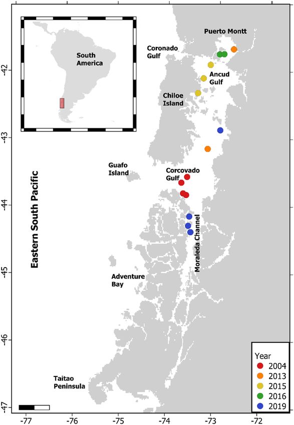
www.nature.com/scientificreports/
Integrating movement and species distribution models. Results from a previous SDM were used
for assessing spatial overlap between blue whale distribution and marine traffic. Briefly, this model consisted
of a Bayesian binomial N-mixture model used to model blue whale groups counts in line-transect data (2009,
2012 and 2014), using distance sampling techniques and oceanographic covariate d ata16. Using an 8 × 8 km grid
spatial predictions of blue whale density at each grid-cell i (Ni) were generated for eight years (2009–2016) and
averaged into a single layer. To integrate outputs from movement models and SDM the relative probability of
encountering a whale (RPEW) was calculated as follows
Ni ν1i
RPEW i = n 1
.
i=1 (Ni νi )
RPEWi assumes that the probability of encountering whales increases with predicted d ensity39,69. Here we
consider behavior might also be part of this function as slow and less persistent movement (ARS) will result in
more time spent (1/νi) allocated to each grid-cell i relative to all other grid cells n. As Ni, had a spatial resolution
of 8 × 8 km, we resampled the νi grid to match the coarser grid resolution prior to any calculation, using the
mean of aggregated grid-cells.
Defining spatial overlap with marine traffic. A quantitative measure of risk associated to vessel traf-
fic can be considered as a monotonic function of the number of vessels and the probability of encountering a
whale39,70. As described above, the relative amount of time allocated to each grid-cell can be obtained from 1/νi.
Therefore, as a measure of risk we calculated the relative probability of vessel encountering whale (RPVEW)39,69
by combining N i, νi and V
Di as follows.
Pw i Pt i Pv i
RPVEW i = n
i=1 (Pw i Pt i Pv i )
where Pw i = n Ni corresponds to the probability of observing a whale within each grid-cell i relative to all
i=1 (Ni ) 1
other grid cells n, Pt i = n
νi
1 corresponds to the time allocated to each grid-cell i relative to all other grid
i=1 ( νi )
cells n, and Pv i = n VDi corresponds to the observed number of vessels within grid-cell i relative to all other
i=1 (VDi )
grid cells n. fleets. Finally, to generate quantitative estimates on the degree of overlap between blue whale distri-
bution and vessel traffic we used the Shoener’s D and Warren’s I similarity s tatistics71. These statistics range from
0, indicating no overlap, to 1, indicating distributions are identical. To use these statistics, the variables Ni times
1/νi and VDi were rescaled to range between 0 and 1 and inputted to the nicheOverlap function from the R
package dismo72,73. A schematic representation of our workflow can be found as a Supplementary Figure S5
online.
Statement of approval. The tagging methods employed in this study were approved by the Institutional
Animal Care and Use Committee of the National Marine Mammal Laboratory of the Alaska Fisheries Science
Center, National Marine Fisheries Service, U.S. National Oceanic and Atmospheric Administration. All methods
employed in this study were carried out in accordance with guidelines from Subsecretaría de Pesca y Acuicultura
(SUBPESCA), which provided full authorization to undertake this research through resolution #2267 of the
Chilean Ministry of Economy and Tourism.
Results
Tracking duration for instrumented whales while within the study area ranged from 8.1 to 105 days (mean = 52.03,
sd = 29.3, median = 48.7), yielding tracks that ranged from 49 to 1,728 locations (mean = 460.27, sd = 582.36,
median = 140) used for modelling (after filtering, Table 1). In general, whales tended to remain in very localized
coastal areas, where high productivity occurs during each austral spring (Fig. 2). No instrumented individuals
departed from NCP until the onset of austral autumn–winter months (April-July)14. Pearson correlation analyses
showed that none of the used covariates were strongly correlated (r < 0.5, p < 0.01). Except for one instrumented
whale (ID#12), all animals showed a significant positive correlation between σt and DAHCC, six animals showed
a significant negative correlation between σt and thermal gradients (Table 1). These results imply a clear pattern
of whales reducing their velocities near areas that were highly productive during spring each year and/or where
higher thermal gradients occur. The relationship with SST was less clear as three individuals showed a significant
negative correlation and five a significant positive one (Table 1).
Regarding correlations between βt and environmental covariates, it was expected that whenever significant,
they would present the opposite sign of those that were significant regarding σt, rendering a continuum between
ARS and transit behavior. This was the case for three individuals with respect to DAHCC (ID#s1, 4 and 8), four
individuals with respect to SST (ID#s 1, 4, 8 and 11) and one individual with respect to thermal gradients (ID#8,
Table 1). Interestingly, two individuals showed the same signal in their correlation between DAHCC and βt, as
well as, between DAHCC and σt (ID# 11 and 15). The same occurred for one individual regarding SST (ID#9)
and one individual regarding thermal gradients (ID#13, Table 1).
Post hoc definition of behavioral states showed the expected occurrence of both transit and ARS behavior.
However, it also showed the occurrence of intermediate behavioral states at locations associated with low speed
and high persistence and vice versa (Fig. 2). These types of intermediate behaviors were more predominant in
individuals tagged in 2016 and 2019.
Scientific Reports | (2021) 11:2709 | https://doi.org/10.1038/s41598-021-82220-5 5
Vol.:(0123456789)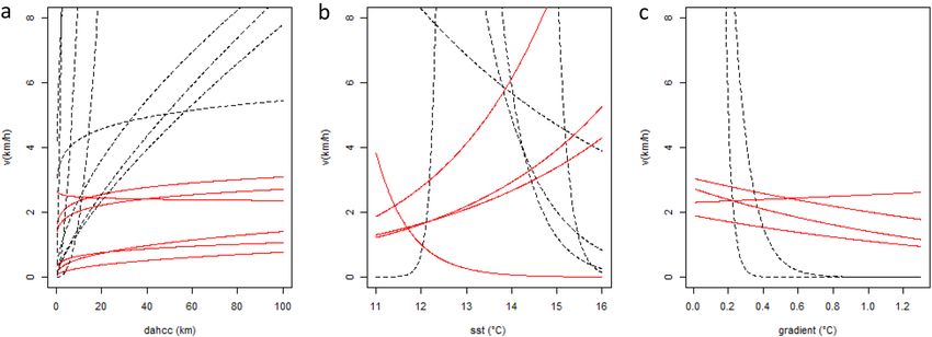
Vol:.(1234567890)
Scientific Reports |
log(σ)
Intercept DAHCC SST Thermal gradient log(sd)
ID Date locs Tracking days Estimate SE Estimate SE p value Estimate SE p value Estimate SE p value Estimate SE
1 2004-02-13 128 75 12.64 0.16 1.76 0.11 < 0.001 − 1.42 0.3 < 0.001 0.12 0.14 0.39 − 9.51 1010
2 2004-02-19 119 62.7 9.6 0.24 0.79 0.17 < 0.001 − 0.09 0.15 0.5 − 0.08 0.12 0.5 − 1.24 0.07
3 2004-02-12 110 36 9.09 0.16 0.43 0.13 < 0.001 − 0.22 0.08 < 0.01 − 0.05 0.11 0.6 − 1.45 0.11
(2021) 11:2709 |
4 2004-02-18 140 47.6 8.74 0.17 0.38 0.1 < 0.001 − 0.27 0.09 < 0.01 − 0.01 0.08 0.95 − 1.12 0.05
5 2013-04-01 304 45.1 8.86 0.08 0.29 0.06 < 0.001 0.1 0.06 0.08 0.08 0.06 0.23 − 0.93 0.02
6 2013-04-23 68 8.1 12.9 0.43 2.2 0.3 < 0.001 0.45 0.24 0.06 0.53 0.42 0.2 − 1.8 0.34
www.nature.com/scientificreports/
7 2015-04-17 314 48.7 8.7 0.12 0.61 0.08 < 0.001 − 0.04 0.06 0.46 − 0.8 0.06 0.19 − 1.17 0.03
8 2015-04-13 130 21.6 12.35 0.3 2.97 0.18 < 0.001 1.69 0.18 < 0.001 − 0.44 0.13 < 0.001 − 1.6 0.12
9 2015-04-09 49 17.1 9.5 0.28 0.56 0.21 < 0.01 0.3 0.13 < 0.05 − 1.28 0.41 < 0.01 − 8.5 173
10 2016-04-04 129 20.1 10.61 0.23 1.16 0.10 < 0.001 − 0.16 0.1 0.11 0.01 0.1 0.9 − 1.15 0.06
11 2016-04-05 1710 105.2 8.85 0.07 0.21 0.03 < 0.001 0.09 0.03 < 0.01 − 0.09 0.03 < 0.05 − 1.62 0.02
12 2019-02-03 649 100 8.19 0.05 0.05 0.11 0.6 0.26 0.04 < 0.001 − 0.11 0.05 < 0.05 − 1.8 0.06
13 2019-02-06 1122 71.4 8.3 0.07 0.19 0.04 < 0.001 0.31 0.03 < 0.001 − 0.08 0.03 < 0.05 − 10.1 291
14 2019-04-27 204 49.1 8.04 0.07 0.71 0.30 < 0.05 − 0.02 0.07 0.72 0.06 0.07 0.4 − 1.02 0.04
15 2019-02-09 1728 72.7 9.04 0.08 0.38 0.03 < 0.001 − 0.02 0.03 0.50 − 0.08 0.03 < 0.01 − 1.76 0.03
log(β)
Intercept DAHCC SST Thermal gradient
ID Date locs Tracking days Estimate SE Estimate SE p value Estimate SE p value Estimate SE p value
1 2004-02-13 128 75 − 1.23 0.6 − 0.53 0.19 < 0.01 6.79 0.43 < 0.001 0.79 0.3 < 0.01
2 2004-02-19 119 62.7 1.86 2.28 − 0.79 1.13 0.49 3.22 1.25 < 0.01 0.08 0.58 0.9
3 2004-02-12 110 36 0.82 0.98 0.22 0.46 0.64 − 0.11 0.49 0.83 1.005 0.63 0.09
https://doi.org/10.1038/s41598-021-82220-5
4 2004-02-18 140 47.6 0.64 0.99 − 1.29 0.42 < 0.01 1.31 0.56 < 0.05 − 0.09 0.3 0.76
5 2013-04-01 304 45.1 4 – – – – – – – – – –
6 2013-04-23 68 8.1 3.5 1.12 – – – – – – – – –
7 2015-04-17 314 48.7 3.34 0.74 0.08 0.32 0.8 1.46 0.33 < 0.001 − 0.25 0.24 0.31
8 2015-04-13 130 21.6 3.36 1.12 − 1.00 0.31 < 0.001 − 3.33 0.39 < 0.001 4.86 0.48 < 0.001
9 2015-04-09 49 17.1 − 1.39 0.37 0.36 0.35 0.3 0.93 0.17 < 0.001 − 0.36 0.38 0.35
10 2016-04-04 129 20.1 4 – – – – – – – – – –
11 2016-04-05 1710 105.2 1.88 0.17 0.49 0.07 < 0.001 − 0.37 0.13 < 0.01 − 0.15 0.12 0.21
12 2019-02-03 649 100 1.31 0.25 − 1.54 1.37 0.26 0.51 0.33 0.13 − 0.09 0.36 0.8
13 2019-02-06 1122 71.4 0.84 0.29 0.22 0.13 0.10 − 0.17 0.11 0.10 − 0.20 0.09 < 0.05
14 2019-04-27 204 49.1 3.57 0.9 − 5.7 3.58 0.11 0.54 0.65 0.41 0.85 0.68 0.21
15 2019-02-09 1728 72.7 2.04 0.2 0.4 0.08 < 0.001 0.05 0.15 0.74 − 0.15 0.1 0.13
Table 1. Parameters estimations for each individual whale (log scale). Individual ID, tag deploying date, number of available locations (locs) and tracking days are provided for each whale.
Missing values for parameters estimating variation in log(β) represent the cases where this was considered as a single parameter instead of a random variable. For each covariate estimates,
6
standard errors (SE), and p values are provided for each parameter. Bold value indicates statistically significance p < 0.05www.nature.com/scientificreports/
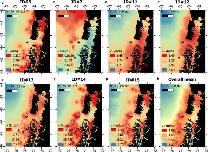
Prediction curves for νt based on covariate variation provided unrealistic predictions for individuals for
which a relatively small number of locations were available (< 200 locations, Fig. 3). For this reason, we only
generated spatial predictions of νt (Fig. 4) for individuals having tracks with more than 200 locations (ID#s 5,
7, 11, 12, 13, 14 and 15). Interindividual variation was observed regarding absolute values for νt, indicating that
some whales moved, in general, faster and in a more persistent manner (Fig. 4 b,c,e) than others, and also in
terms of where their lowest values (ARS behavior) were expected. Despite this individual variation, some areas
were consistently depicted as having the lowest values for νt, which are highlighted when the spatial predictions
for these seven whales were averaged into an overall mean (Fig. 4h). Spatial predictions on RPEW highlighted
areas of aggregation for blue whales in NCP, mainly located in the western part of Chiloe Island, Ancud Gulf,
Adventure Bay and northern Moraleda Channel (Fig. 5).
VD absolute values were highest for the aquaculture fleet (range:0–78.4) followed by artisanal fishery (0–13.9),
transport (range: 0–8) and industrial fishery (range: 0–1.9) fleets. The number of active vessels per day was high-
est for the aquaculture fleet (range: 602–729), followed by the artisanal fishery (range: 37–76), transport (range:
6–57) and industrial fishery (range: 1–13) fleets. Although the four fleets studied here showed spatial variation
on RPVEW, all of them coincided in a high probability of whales interacting with vessels throughout the Chiloe
inner sea (Fig. 6). Among the four fleets studied the artisanal fishing fleet showed the highest overlap with blue
whale distribution patterns (D = 0.34; I = 0.64). The industrial fishery (D = 0.28; I = 0.48), aquaculture (D = 0.24;
I = 0.46) and transport (D = 0.23; I = 0.45) fleets showed similar lower overlap (Fig. 6).
Discussion
Blue whale habitat selection and priority areas for conservation. Understanding the environmen-
tal drivers of blue whale habitat s election16,17 is paramount for defining priority areas for its conservation and
developing recommendations for marine spatial p lanning11,74. In pursuing this goal, our setting combined pre-
vious SDM fit to line-transect data with a movement model fit to telemetry data in a complementary manner.
Telemetry data supports the spatial pertinence of previously defined areas for assessing blue whale abundance
and distribution patterns through ship-borne surveys. Although, some whales performed brief excursions to
adjacent offshore waters, they tended to remain within the NCP coastal areas during most of the tracking time,
which in two cases extended for up to 3 months (Table 1). Potential caveats to this approach include tagging
location bias (i.e. only performed in coastal waters, Fig. 1) and sampling size, which should be overcome through
the ongoing tagging program.
Previous SDM16 showed that spring productivity and, secondarily, thermal fronts were important covariates
for predicting blue whale densities. Results here show that the same covariates selected by SDM are important for
understanding blue whale’s movement patterns. As with the aforementioned SDM, DAHCC was the most preva-
lent covariate retained in our models, which combined with thermal gradients, displayed an unequivocal pattern
in their correlation with σt. This is, whales tended to reduce their velocity near areas of high primary productivity
that had occurred during austral spring and where strong thermal gradients take place (Table 1, Fig. 3a). As with
many other large whale species, worldwide abundance and distribution patterns of blue whales have been linked
to predictable highly and seasonally productive waters associated to high chlorophyll-a, among other proxies
for enhanced p roductivity19,20,24,75–78. Nevertheless, as blue whales feed almost exclusively on krill, temporal lags
are expected to occur between seasonally high primary productivity, euphausiids early life-history stage pro-
cesses (e.g. larval recruitment), the peak in adult euphausiid densities and the peak in whale a bundance17,20,78.
Refining our understanding of how temporal lags relate chlorophyll-a to euphausiid spatial patterns and then
to blue whale distribution remains a pending t ask79,80, especially considering that euphausiid spatial ecology in
the NCP is poorly understood49,81.
Although spring chlorophyll-a appears to be a suitable general proxy for blue whale prey availability in the
NCP, whales are expected to respond in a much more complex manner to environmental heterogeneity. Previ-
ously, blue whale density in the NCP was found to be higher near areas of thermal front r ecurrence16. By using
telemetry data, we were able to refine the assessment scale and test whether blue whales responded to daily
changes in thermal gradients. Despite the relatively coarse resolution of Argos data, we were able to find evidence
for behavioral response in six whales while traversing thermal gradients of less than 1 °C (Fig. 3c). This may
even represent an underestimation given the reported response of blue whales to gradients as low as 0.03 °C82.
Thus, our results provide additional support on the relevance of coarse to meso-scale thermal gradients when
shaping marine predator distribution16,23,82,83. The underlying mechanism for this pattern, however, is not clear,
as thermal fronts might be responsible for increasing prey availability by boosting local productivity and/or by
aggregating prey p atches22–25,83,84. Within the NCP, both processes are likely to be tightly coupled. The influence
of fresh waters rich in silicic acid, among other nutrients, from high river discharges due to glacier melt and
heavy rain, fertilize the photic zone by mixing with macronutrient-loaded oceanic deep w ater46,49,81,85,86. This
large fresh water input in conjunction with higher irradiance reaching the surface during spring and summer,
wind stress, tide and complex bottom topography promotes alternating processes of vertical and horizontal
stratification/mixing of the water column, enhancing primary production as well as plankton a ggregation87–89.
In this context, areas selected by blue whales in the NCP might not just be of high biological productivity, but
where frontal dynamics lead to highly concentrated prey patches.
SST presented an equivocal pattern regarding blue whale movement patterns, suggesting a preference for
colder waters in four individuals and the opposite in four other individuals (Table 1, Fig. 3b). This might be a
temporal issue if whales in some years/seasons found their prey in colder/warmer waters. For instance, Ancud
Gulf tends to present higher temperatures during spring and summer than the Corcovado Gulf as the latter rep-
resents the main entrance path for sub-superficial oceanic colder waters into the Chiloe inner sea. Alternatively,
Scientific Reports | (2021) 11:2709 | https://doi.org/10.1038/s41598-021-82220-5 7
Vol.:(0123456789)www.nature.com/scientificreports/
Figure 2. Behavioral variation for tagged whales. Panels (a–e) summarize results for 2004, 2013, 2015, 2016 and
2019, respectively and panel f combines all tracks. Red to blue four-color ramp indicates the percentile to which
each location belongs regarding variation in σt and 3/βt (persistence). By using the medians, the four possible
combinations are presented as a posteriori behavioral state identification. Locations jointly holding values of
σt and 3/βt below their medians across all whales (low s and low p) can be considered ARS behavior, while the
opposite (high s and high p) can be considered transit. Blue (far) to yellow (close) color ramp in the background
indicates variation in standardized distance to areas of high chlorophyll concentration (DAHCC) in log scale,
which was the most consistent covariate shaping blue whale movement patterns in this study. Data layers
(including maps) were created in R ver. 4.0.2 (www.r-project.org) and ensembled in QGIS ver. 3.8.0 (www.qgis.
org) for final rendering. Maps were created using data on bedrock topography from the National Centers for
Environmental Information (https://maps.ngdc.noaa.gov/viewers/grid-extract/index.html). Values above 0 were
considered land coverage.
the lack of a clear trend in observed blue whale movement patterns regarding SST might be the result of a prefer-
etect76.
ence for intermediate temperatures that linear predictors failed to d
Blue whales appear to respond to dynamic water-column processes by performing continuous behavioral
changes without necessarily departing from relatively discrete areas (e.g. Ancud Gulf and Moraleda Channel,
Fig. 2). For instance, whales ID#11, ID#13 and ID#15 presented a higher probability of reducing their velocity
nearby areas of high productivity and strong thermal gradients, a higher probability of increasing persistence
nearby areas of high productivity (for whales ID#11 and ID#15, Table 1), and all three spent from one to 3 months
within specific micro-basins (Ancud Gulf and Moraleda Channel). This suggests that both transit-like and ARS
behaviors co-occur spatially, temporarily oscillating with the suitability of foraging conditions.
Higher blue whale densities observed in the same areas where tagged individuals presented ARS behavior in
a previous study16 could have been attributed to multiple individuals entering and leaving these areas. However,
the results presented here show that instrumented blue whales concentrate in relatively discrete areas for extended
periods of time (up to 3 months) searching for and exploiting available resources. The limited movement elicited
by blue whales might be regarded as an indicator of low interspecific competition, considering that their popu-
lation abundance is still estimated to be considerably below pre-whaling levels16,90,91. Other mechanisms like
dominance92 and predator a voidance93, have been purported to explain limited animal movement. Thus, other
factors should be considered in the future for understanding other dimensions of blue whales’ habitat selection
process, as well as temporal variations on it.
Scientific Reports | (2021) 11:2709 | https://doi.org/10.1038/s41598-021-82220-5 8
Vol:.(1234567890)www.nature.com/scientificreports/
Figure 3. Prediction curves indicate expected variation in long-term velocity (νt) in relation to environmental
covariates, (a) distance to areas of high chlorophyll concentration (DAHCC) in log scale, (b) sea surface
temperature (SST) and c) thermal gradients. Red lines indicate predictions for whales exhibiting more than 200
locations (ID#s 5, 7, 11, 12, 13, 14 and 15) and black lines correspond to those with less locations available.
Figure 4. Spatial predictions of expected long-term velocity (νt) responses in the entire study area, for every
instrumented whale with more than 200 locations (panels a–g). The bottom right panel (h) shows the overall
mean for all seven individuals. Data layers (including maps) were created in R ver. 4.0.2 (www.r-project.org)
and ensembled in QGIS ver. 3.8.0 (www.qgis.org) for final rendering. Maps were created using data on bedrock
topography from the National Centers for Environmental Information (https://maps.ngdc.noaa.gov/viewers/
grid-extract/index.html). Values above 0 were considered land coverage.
Scientific Reports | (2021) 11:2709 | https://doi.org/10.1038/s41598-021-82220-5 9
Vol.:(0123456789)www.nature.com/scientificreports/
Figure 5. Relative probability of encountering a blue whale (RPEW). This integrates the output of the
movements and species distribution models for areas within 25 km from shore. Data layers (including the map)
were created in R ver. 4.0.2 (www.r-project.org) and ensembled in QGIS ver. 3.8.0 (www.qgis.org) for final
rendering. Map was created using data on bedrock topography from the National Centers for Environmental
Information (https://maps.ngdc.noaa.gov/viewers/grid-extract/index.html). Values above 0 were considered
land coverage.
Independently, both SDM and movement models predictions, highlighted similar areas of aggregation for
blue whales in NCP based on observed oceanographic conditions (see Supplementary Fig. S5 online). These are
clearly delimited by our RPEW map and considered Ancud Gulf, the Western coast of Chiloe Island, Corcovado
Gulf / Moraleda Channel (CGMC), and Adventure Bay (Figs. 1 and 5). As previous SDMs were restricted to
areas within 25 km from shore, some offshore areas visited by blue whales were not considered during RPEW
computation. However, as the overall tendency to remain in coastal waters by instrumented whales was clear
(Fig. 2f), we consider RPEW to be adequate.
Quantifying overlap with vessel traffic. For Chile, detailed and freely available vessel traffic data as
those used here are limited to recent years (2019–2020), precluding long term assessments on vessel traffic
spatiotemporal variation95. Although limited to 10 months of data, results showed little intra-fleet variation for
the transport and aquaculture vessel activities, as well as, for those occurring in the inner sea for both fishing
fleets (see Supplementary Figs. S1–S4 online). This was expected as transport and logistic support operations
from aquaculture operations are less variable than the shifting resource-tracking operations of fishing vessels. In
addition, the inner waters concentrate obligated marine corridors for entering/leaving the area which are used
similarly regardless of vessel type. Henceforth, our estimates are expected to adequately reflect general vessel
traffic patterns for each fleet but inspecting possible temporal variation in these patterns should be pursued in
the future.
The four different vessel fleets considered here elicited differences in VD values and their spatial use of the
study area (Fig. 6). While artisanal and industrial fishing fleets utilize inner waters to the east and open waters
to the west of the study area, aquaculture and transport fleets are mainly constrained to inner waters (Fig. 6).
According to Chilean legislation, the artisanal fishing fleet is restricted to operate within 5 nm (9.3 km) from the
coast in open and inner waters while the industrial fishing operations are to be performed beyond this area to the
West. This might explain the artisanal fishing fleet´s high score on the similarity statistics, indicating the largest
degree of overlap with blue whale coastal distribution. In other words, this fleet distributes the RPVEW more
Scientific Reports | (2021) 11:2709 | https://doi.org/10.1038/s41598-021-82220-5 10
Vol:.(1234567890)www.nature.com/scientificreports/
Figure 6. Top panels show vessel density (VD) as the mean number of vessels visiting each 8 × 8 km grid-cell
per day, for the industrial fishery (a), artisanal fishery (b), aquaculture (c) and transport (d) fleets. Note the
large difference in color bar increments for the aquaculture fleet. Bottom panels show the relative probability
of vessel encountering whale (RPVEW) for the industrial fishery (e), artisanal fishery (f), aquaculture (g) and
transport (h) fleets. The data of the different fleets are provided by the Chilean national services of fisheries and
aquaculture, (SERNAPESCA) and are freely available at www.sernapesca.cl. Data layers (including maps) were
created in R ver. 4.0.2 (www.r-project.org) and ensembled in QGIS ver. 3.8.0 (www.qgis.org) for final rendering.
Maps were created using data on bedrock topography from the National Centers for Environmental Information
(https://maps.ngdc.noaa.gov/viewers/grid-extract/index.html). Values above 0 were considered land coverage.
homogeneously matching blue whale distribution, while other fleets concentrate only at specific areas (lower
degree of overlap). In comparison with results presented here, a study using the same overlap statistics, showed
a higher degree of overlap between vessels and three species of cetaceans in the Mediterranean S ea73. This was
expected as the Mediterranean Sea is a high intensity vessel traffic a rea96. However, most of the marine traffic
recorded in that study (73.3%) corresponded to small sailing boats, suggesting low probabilities of lethal ship-
strikes in general but pinpointing that shipping routes (where larger vessels navigate) might pose higher risk. This
brings forward the fact that spatial overlap is just one of the factors affecting collision risk and its outcome, with
vessel density, speed and size also contributing to i t39,40,97. Although the industrial fishing fleet presents a lower
degree of spatial overlap with blue whales and the lowest number of operating vessels, industrial vessels might
yield a higher probability of lethal interactions if they occur, due to larger vessel size. This fleet also presented a
particular pattern of high RPVEW values off Adventure Bay (Fig. 6).
With up to 729 active vessels operating per day (83% of the total) and up to 78 vessels per day crossing a
single grid-cell (VD), aquaculture fleet corresponds to the largest and most densely distributed fleet in the NCP.
Hence, while RPVEW predictions highlights the specific areas where interactions are more likely to occur for
each vessel fleet, in absolute terms, it is possible that the aquaculture fleet represents the major driver of negative
vessel-whale interactions in NCP.
When considering results from all fleets together it is clear that the inner waters largely concentrate higher
VD and high RPVEW values for all fleets (Fig. 6). This area holds the largest number of human settlements
in the NCP and the main port pertaining to the regional capital, Puerto Montt, raising concerns for potential
collisions, behavioral disturbance and/or heavy noise e xposure38,94,98–101 for blue whales there. Although, no
systematic monitoring or registering protocol exists in this region, local authorities’ statements and the local
press have documented at least three large whale mortality events linked to vessel collisions in the NCP (two
Scientific Reports | (2021) 11:2709 | https://doi.org/10.1038/s41598-021-82220-5 11
Vol.:(0123456789)www.nature.com/scientificreports/
blue whales and one sei whale), with two occurring nearby Puerto Montt and the other one at CGMC (Fig. 5).
The ability of blue whales to avoid approaching vessels appears to be limited to relatively slow descents/ascents,
with no horizontal movements away from a vessel102,103, therefore, collision events might pose significant threats
to survival and r ecovery97 for this endangered population. As inner waters of NCP might be considered, at the
time, the spot of higher relative and absolute probabilities of negative interactions between blue whales and
vessels, management actions are urgently needed to be implemented. For now, the most effective way to reduce
collision risk is to keep whales and vessels apart, either in space or time, and where/when this is not possible,
other measures (such as speed regulation) can be sought and applied singularly or in combination, considering
variations in vessel activity and whale´s d istribution40,102,104, as data become available. In addition, it is important
to acknowledge that all analyses performed here were restricted to vessels carrying transponders and legally
mandated to submit position data. Therefore, several vessels types operating in the area that could contribute
to collision risk (e.g. international cargo and tankers, cruiseliners, as well as artisanal, recreational and military
vessels) are currently unaccounted for.
Because widely migratory species, such as the blue whale, do not recognize political boundaries, it is of great
importance to identify the location of corridors and critical areas where they perform their vital activities (i.e.,
feed, migrate, breed, calve) to provide baseline information for their conservation. Efforts must be implemented
at the local, national and international scales if success is to be reached, as ESP blue whale population recovery
might be jeopardized by the loss of even a few individuals a year16 after being severely depleted by the whaling
industry during the 20th Century.
Modelling approach. One of the main differences between our modelling approach and previously pub-
lished SSMs is in that behavioral variation that arises from the dependence on time-varying parameters (σt and
βt) rather than switches in discrete pre-determined behavioral states30,31,65,107. While the latter approach allows
formal prediction, testing on the spatio-temporal occurrence of known behavioral modes (e.g. areas where ARS
is likely to occur), time-varying approaches permit investigating variation in movement patterns that cannot, or
are not desired to be, categorized a priori65,107,108. This poses a significant advantage in cases where animal move-
ment fails to conform to the usual transit/ARS binary view. For instance, a previous w ork14 fitted a switching
SSM to most of the data we analyzed here and found that transit states were very rare within the NCP. In agree-
ment with this, our results show that ca. 75% of all whale estimated locations presented persistence values lower
than 1.6 h, which is consistent with the biological expectation of whales primarily engaged in foraging related
CP12. In this scenario, attempting to explore the effect of environmental variables on switching
activities within N
probability between ARS and transit s tates76 would have been difficult, as very few locations and their associated
covariates would have been available for the transit state. By exploring changes in movement parameters, we can
assess how animals’ velocity and/or persistence respond to environmental covariates without the need of further
assumptions. Following the transit/ARS rationale of conventional switching SSMs, one would expect that if a
covariate is correlated with σt it also would be with βt, but with an opposite sign. That is, at certain covariate
values an animal’s velocity and persistence are likely to decrease indicating ARS behavior, as was the case for
several individuals and variables (Table 1). However, this does not need to always be the case, as shown by whales
ID#11 and ID#15, which reduced their velocity near areas of high productivity in conjunction with increased
persistence (Table 1). In general, this might occur because both transit and ARS behavior co-occur in similar
areas with respect to DAHCC but differ in other variables (SST and thermal gradients). Nonetheless, alternative
explanations for other behaviors, apart from transit/ARS, might arise. For instance, short-lived chasing bursts
(escorting-like behavior) has been described for the NCP109 , which are expected to present high velocities but
not necessarily high persistence. On the other hand, slow persistent behavior, mostly present in whales tagged
in years with the highest data transmission throughput (2016–2019, Fig. 2d–e, Table 1), might be explained by
the ratio of the location error relative to the scale of movement. Thus, if short time periods separate two or more
locations with limited movement, high persistence might arise from negligible variation in both speed and loca-
tion, as observation error increases disproportionately relative to the scale of the movement process.
Overall, our modelling approach accounted for observational error and allowed for the incorporation of
environmental covariates to inform movement parameters without the need for regularization of location data
into fixed time intervals30,65, all in one single step. By fitting the model through the R package “TMB” analysis
took an average of 60.5 s to run (range: 2.6–310.6, processor: Intel Core i7-7700HQ at 2.8 GHz, RAM: 32 GB)
which is a significant advantage when processing large amounts of data.
Conclusions
Blue whale movement patterns agree with previous studies on their distribution, highlighting the importance
of coastal waters and reinforcing our knowledge about primary production and thermal fronts as important
environmental drivers for this species´ habitat selection process in the NCP. Considering defined priority areas
for blue whale conservation in the area, those located at inner waters concentrated the highest probabilities of
whales interacting with vessels. Among the studied vessel fleets, the unparalleled size of the aquaculture fleet
indicates this could play a decisive role in modulating potential negative vessel-whale interactions within NCP.
The results of this study clearly pinpoint specific areas where management actions are urgently needed, especially
considering the undetermined number of vessels strikes and levels of noise exposure in the region. This infor-
mation should be considered by Governmental and International organizations to inform, design, and rapidly
implement mitigation action using existing national and international conservation instruments.
Scientific Reports | (2021) 11:2709 | https://doi.org/10.1038/s41598-021-82220-5 12
Vol:.(1234567890)www.nature.com/scientificreports/
Data availability
C + + /TMB code for fitting the model (CTCRW_matrix_cov.cpp), raw telemetry data and accompanying covari-
ate data are available as Supplementary Information.
Received: 26 August 2020; Accepted: 18 December 2020
References
1. Hays, G. C. et al. Key questions in marine megafauna movement ecology. Trends in Ecol. Evol. 0 (2016).
2. Nathan, R. et al. A movement ecology paradigm for unifying organismal movement research. PNAS 105, 19052–19059 (2008).
3. Spiegel, O., Leu, S. T., Bull, C. M. & Sih, A. What’s your move? Movement as a link between personality and spatial dynamics in
animal populations. Ecol. Lett. 20, 3–18 (2017).
4. Hussey, N. E. et al. Aquatic animal telemetry: a panoramic window into the underwater world. Science 348, 1255642 (2015).
5. Kays, R., Crofoot, M. C., Jetz, W. & Wikelski, M. Terrestrial animal tracking as an eye on life and planet. Science 348, aaa2478
(2015).
6. Cooke, S. J. Biotelemetry and biologging in endangered species research and animal conservation: relevance to regional, national,
and IUCN Red List threat assessments. Endanger. Species Res. 4, 165–185 (2008).
7. Costa, D. P., Breed, G. A. & Robinson, P. W. New insights into pelagic migrations: implications for ecology and conservation.
Annu. Rev. Ecol. Evol. Syst. 43, 73–96 (2012).
8. Žydelis, R. et al. Dynamic habitat models: using telemetry data to project fisheries bycatch. Proc. R. Soc. Lond. B: Biol. Sci. 278,
3191–3200 (2011).
9. Hays, G. C. et al. Translating marine animal tracking data into conservation policy and management. Trends Ecol. Evol. 34,
459–473 (2019).
10. Cooke, J. IUCN Red List of Threatened Species: Blue Whale. IUCN Red List of Threatened Species. https://www.iucnredlist.org/
en (2018).
11. Hucke-Gaete, R., Moro, P. L. & Ruiz, J. Conservando el mar de Chiloé, Palena y las Guaitecas. Síntesis del estudio Investigación
para el desarrollo de Área Marina Costera Protegida Chiloé, Palena y Guaitecas. Valdivia, Chile: Universidad Austral de Chile
and Lucas Varga para The Natural Studio. Accessed June 30, 2014 (2010).
12. Hucke-Gaete, R., Osman, L. P., Moreno, C. A., Findlay, K. P. & Ljungblad, D. K. Discovery of a blue whale feeding and nursing
ground in southern Chile. Proc. R. Soc. Lond. B 271, S170–S173 (2004).
13. Buchan, S. J., Stafford, K. M. & Hucke-Gaete, R. Seasonal occurrence of southeast Pacific blue whale songs in southern Chile
and the eastern tropical Pacific. Mar. Mamm. Sci 31, 440–458 (2015).
14. Hucke-Gaete, R. et al. From Chilean Patagonia to Galapagos, Ecuador: novel insights on blue whale migratory pathways along
the Eastern South Pacific. PeerJ 6, e4695 (2018).
15. Torres-Florez, J. P. et al. First documented migratory destination for eastern South Pacific blue whales. Mar. Mam. Sci. https://
doi.org/10.1111/mms.12239(2015).
16. Bedriñana-Romano, L. et al. Integrating multiple data sources for assessing blue whale abundance and distribution in Chilean
Northern Patagonia. Divers. Distrib. https://doi.org/10.1111/ddi.12739 (2018).
17. Buchan, S. J. & Quiones, R. A. First insights into the oceanographic characteristics of a blue whale feeding ground in northern
Patagonia, Chile. Mar. Ecol. Prog. Ser. 554, 183–199 (2016).
18. Atkinson, A., Siegel, V., Pakhomov, E. & Rothery, P. Long-term decline in krill stock and increase in salps within the Southern
Ocean. Nature 432, 100–103 (2004).
19. Branch, T. A. et al. Past and present distribution, densities and movements of blue whales Balaenoptera musculus in the Southern
Hemisphere and northern Indian Ocean. Mam. Rev. 37, 116–175 (2007).
20. Croll, D. A. et al. From wind to whales: trophic links in a coastal upwelling system. Mar. Ecol. Prog. Ser. 289, 117–130 (2005).
21. Zerbini, A. N. et al. Baleen whale abundance and distribution in relation to environmental variables and prey density in the
Eastern Bering Sea. Deep Sea Res. Part II 134, 312–330 (2016).
22. Acha, E. M., Mianzan, H. W., Guerrero, R. A., Favero, M. & Bava, J. Marine fronts at the continental shelves of austral South
America: Physical and ecological processes. J. Mar. Syst. 44, 83–105 (2004).
23. DoniolValcroze, T., Berteaux, D., Larouche, P. & Sears, R. Influence of thermal fronts on habitat selection by four rorqual whale
species in the Gulf of St, Lawrence. Mar. Ecol. Prog. Ser. 335, 207–216 (2007).
24. Littaye, A., Gannier, A., Laran, S. & Wilson, J. P. F. The relationship between summer aggregation of fin whales and satellite-
derived environmental conditions in the northwestern Mediterranean Sea. Remote Sens. Environ. 90, 44–52 (2004).
25. Lutjeharms, J. R. E., Walters, N. M. & Allanson, B. R. Oceanic frontal systems and biological enhancement. In Antarctic Nutrient
Cycles and Food Webs 11–21 (Springer, Berlin, Heidelberg, 1985). doi:https://doi.org/10.1007/978-3-642-82275-9_3.
26. Acevedo-Gutiérrez, A., Croll, D. A. & Tershy, B. R. High feeding costs limit dive time in the largest whales. J. Exp. Biol. 205,
1747–1753 (2002).
27. Goldbogen, J. A. et al. Prey density and distribution drive the three-dimensional foraging strategies of the largest filter feeder.
Funct. Ecol. 29, 951–961 (2015).
28. Goldbogen, J. A. et al. Mechanics, hydrodynamics and energetics of blue whale lunge feeding: efficiency dependence on krill
density. J. Exp. Biol. 214, 131–146 (2011).
29. Potvin, J., Goldbogen, J. A. & Shadwick, R. E. Passive versus active engulfment: verdict from trajectory simulations of lunge-
feeding fin whales Balaenoptera physalus. J. R. Soc. Interface 6, 1005–1025 (2009).
30. Jonsen, I. D., Flemming, J. M. & Myers, R. A. Robust state–space modeling of animal movement data. Ecology 86, 2874–2880
(2005).
31. Morales, J. M., Haydon, D. T., Frair, J., Holsinger, K. E. & Fryxell, J. M. Extracting more out of relocation data: building move-
ment models as mixtures of random walks. Ecology 85, 2436–2445 (2004).
32. Waerebeek, K. V. et al. Vessel collisions with small cetaceans worldwide and with large whales in the Southern Hemisphere, an
initial assessment. Latin Am. J. Aquat. Mamm. 6, 43–69 (2007).
33. Buschmann, A. H. et al. A review of the impacts of salmonid farming on marine coastal ecosystems in the southeast Pacific.
ICES J. Mar. Sci. 63, 1338–1345 (2006).
34. Niklitschek, E. J., Soto, D., Lafon, A., Molinet, C. & Toledo, P. Southward expansion of the Chilean salmon industry in the
Patagonian Fjords: main environmental challenges. Rev. Aquac. 5, 172–195 (2013).
35. Viddi, F. A., Harcourt, R. G. & Hucke-Gaete, R. Identifying key habitats for the conservation of Chilean dolphins in the fjords
of southern Chile. Aquat. Conserv: Mar. Freshw. Ecosyst. https://doi.org/10.1002/aqc.2553 (2015).
36. Hoyt, E. & Iñiguez, M. Estado del avistamiento de cetáceos en América Latina. WDCS, Chippenham, UK 60 (2008).
37. Colpaert, W., Briones, R. L., Chiang, G. & Sayigh, L. Blue whales of the Chiloé-Corcovado region, Chile: potential for anthro-
pogenic noise impacts. Proc. Mtgs. Acoust. 27, 040009 (2016).
Scientific Reports | (2021) 11:2709 | https://doi.org/10.1038/s41598-021-82220-5 13
Vol.:(0123456789)You can also read