Detection and Mitigation of Transient Instabilities in Multi-Agent Systems and Swarms
←
→
Page content transcription
If your browser does not render page correctly, please read the page content below
i-SAIRAS2020-Papers (2020) 5091.pdf
Detection and Mitigation of Transient Instabilities
in Multi-Agent Systems and Swarms
Saptarshi Bandyopadhyay1 , Vinod Gehlot2 , Mark Balas2 , David S. Bayard1 , Marco B. Quadrelli1
Abstract—We first introduce the novel concept of transient
instabilities in multi-agent systems and swarms, i.e., a small
disturbance leads to increasing-amplitude oscillations throughout
the swarm, which results in a large number of inter-agent
collisions. This instability is dominant in the transient phase of
the system and it does not appear in the steady-state behavior of
the system, as each agent uses Lyapunov-stable feedback control
laws. We present a rigorous definition of transient instability
in swarms, and discuss its key properties. We also present a
sufficient condition to check if a swarm will be transient stable.
We study the behaviour of different control laws under this
condition. We also show how transient instability phenomenon
could impact the dynamics of deployable structures.
Next, we present a novel control architecture that augments the
baseline formation maintenance controller to mitigate transient
instabilities. At its heart, the proposed architecture consists of
a projection operator based estimator disguised as a reference
model that generates collision-free trajectories for the agents to
follow. We present numerical simulation results to demonstrate
the effectiveness of our proposed approaches.
I. I NTRODUCTION
Multi-agent systems and swarms, consisting of formations
or constellations of small satellites or teams of aerial and
ground robots, can be used for a variety of applications in
space, in air, and on ground. It is commonly assumed in the
control theory literature that proving the Lyapunov-stability of
a swarm’s dynamics is sufficient to ascertain the stability of the Figure 1: Motion of a 2D swarm of agents, where each
swarm. In this paper we show that this assumption is incorrect, agent tries to maintain a constant distance with its preceding
i.e., there exist formation geometries/shapes and Lyapunov- agents along both dimensions. A small disturbance in either
stable feedback control laws that can lead to multiple inter- dimension leads to increasing-amplitude oscillations through-
agent collisions within the swarm. out the swarm, which results in a large number of inter-agent
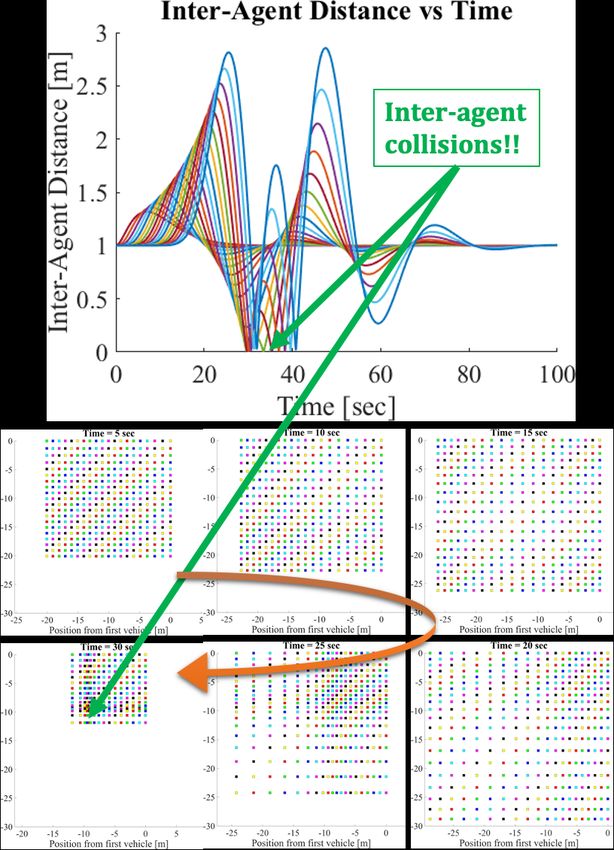
We use the following toy problem to describe the concepts collisions. We define this phenomenon as transient instability.
in this paper. The evolution of a 2-dimensional (2D) swarm
of agents is shown in Fig. 1, where each agent tries to
leads to inter-agent collisions as transient instability. This
maintain a constant distance with its preceding agents along
instability is dominant in the transient phase of the system and
both dimensions. A small disturbance in either dimension leads
it does not appear in the steady-state behavior of the system.
to increasing-amplitude oscillations throughout the swarm,
which results in a large number of inter-agent collisions. Since each agent’s motion is asymptotically stable, all sta-
These oscillations die out with time and the steady-state bility techniques in traditional control theory (like gain/phase
behavior is asymptotically stable. We define this phenomenon margin and root locus for linear systems and Lyapunov theory
of increasing-amplitude oscillations within the swarm that or contraction theory for nonlinear systems) cannot detect
these transient instabilities because each agent’s motion is
1 S. Bandyopadhyay, M. Quadrelli, and D. Bayard are with technically stable according to the standard stability definition
the Jet Propulsion Laboratory, California Institute of Technology, used in traditional control theory.
4800 Oak Grove Dr., MS 198-219, Pasadena, CA, USA
91109, saptarshi.bandyopadhyay@jpl.nasa.gov,
marco.b.quadrelli@jpl.nasa.gov, A. Literature Survey
david.s.bayard@jpl.nasa.gov Transient instabilities were first discovered in one-
2 V. Gehlot and M. Balas are with the Mechanical Engineering De-
partment, Texas A&M University, College Station, Texas, USA 77843, dimensional (1D) vehicle convoys in the 1970s [1], where it is
vinodgehlot@tamu.edu, mbalas@tamu.edu often denoted as string instability. Many mitigation strategies
1i-SAIRAS2020-Papers (2020) 5091.pdf
have been proposed for 1D vehicle convoys in [2]–[4]. A • We first rigorously define transient instabilities in swarms,
recent review paper [5] lists the state-of-the-art results in string and discuss its various features in Section II.
stability of vehicle platoons. • We present a mathematical framework or “theoretical
To our knowledge, this is the first paper to show that such tool” to detect transient instabilities in swarms in Sec-
transient instabilities can also arise in 2D or 3D swarm for- tion II-A. For a special case, we also prove that this tool
mations. The main difficulties in applying the vehicle convoys is a sufficient condition for avoiding transient instabilities
solutions to swarms are as follows: in swarms.
• Swarms are usually deployed in higher dimensions (2D • In Section II-B, we show that the standard Proportional-
and 3D), and the coupling between the dimensions in- Integral-Derivative (PID) control law does not satisfy this
troduces new complexities not discussed in the previous condition for linear systems. In Section II-C, a robust
literature on 1D vehicle convoys. control law [10], previously introduced for non-swarm
• The dynamics of vehicle convoys is usually represented applications, satisfies this condition and always avoids
by linear time-varying equations, hence tools from linear transient instabilities for linear systems.
systems control theory are usually used in the solution ap- • In Section III, we present a transient-stable mitiga-
proach. The dynamics of swarm agents are often nonlin- tion/control approach, which consists of the relative er-
ear (e.g. spacecraft, quadrotor) hence solutions techniques ror feedback controller and the combined projection-
from linear systems control theory cannot be directly based collision-free trajectory generator and the tracking
applied. controller. We present numerical simulation results in
In [6], the authors develop a novel control approach to Section III-A to demonstrate collision-free asymptotic
formation construction and reconfiguration and show that it is stability of the inter-agent relative error dynamics.
possible to satisfy collision-free exponential stability in two- Finally, Section IV concludes the paper.
agent systems. Recently, in [7], the authors develop a unique
control approach to satisfying transient stability using Control II. D ETECTION OF T RANSIENT I NSTABILITY IN S WARMS
Barrier Functions (CBF). Here, the simultaneous problems
of exponential stability and collision-avoidance are posed as In order to understand transient instability in swarms, let us
a Quadratic Program (QP) and solved continuously; it is a first discuss the example in Fig. 1. The indices used in this
centralized control approach. In the comprehensive survey example are described in Fig. 2. Here is a 2D swarm of N × M
of multi-agent algorithms [8], the coordination and control agents, where N, M ∈ N. Each (i, j)th follower agent (shown
algorithms fall into two distinct categories: predictive and in blue) is trying to maintain a constant separation distance
reactive. D ∈ R from the right (i − 1, j)th agent and up (i, j − 1)th agent.
The leader (1, 1)th agent (shown in red) decides the desired
B. Transient Instability in Deployable Structures trajectory of the swarm, that all the follower agents will follow.
A deployable structures can change significantly change The leader+follower agents at the start of each axis (shown
their shape or size, like umbrellas, tensegrity structures, in green) also ensure that the swarm maintains the desired
Origami shapes, scissor-like structures. Advanced deployable trajectory selected by the leader agent.
structures are a high TRL technology and have been used
for a wide variety of applications in space, including solar
panels, booms, large antennae, solar sails, sun shield, etc. and
in missions like NuSTAR, SMAP, MarCO, RainCube and on-
going efforts in missions like Starshade [9], SWOT, NISAR.
We believe that the analogue of the above transient insta-
bilities in swarms can also be found in deployable structures,
which is currently not known. In finite element analysis (for
example, modeled with the Galerkin method), a structure is
modeled with partial differential equations, and discretized as
a mesh of point-masses connected to their neighboring point-
masses by linear or nonlinear springs that approximate the
physical connections. This is analogous to a swarm of agents
that interact with their neighboring agents using control laws.
Hence we need a rigorous theoretical framework to detect and
mitigate these transient instabilities in deployable structures,
which will be the focus of future work. Figure 2: Indices used in the 2D swarm of agents example.
C. Main Contributions Let xi, j (t) = [pi, j,x (t) pi, j,y (t) vi, j,x (t) vi, j,y (t)] denote the state
The main contributions and organization of this paper are of the (i, j)th agent in the swarm at time t, where pi, j,x , pi, j,y
as follows: and vi, j,x , vi, j,y are the positions and velocities of the agent in
2i-SAIRAS2020-Papers (2020) 5091.pdf
the X-axis and Y-axis respectively. The dynamics of the (i, j)th because each agent’s motion is technically stable accord-
follower agent (∀i ∈ {1, . . . , N}, ∀ j ∈ {1, . . . , M}) is given by: ing to the standard stability definition used in traditional
control theory. In other words, if each agent’s motion is
ṗi, j,x (t) = vi, j,x (t), (1)
individually analyzed, then it passes the stability checks
ṗi, j,y (t) = vi, j,y (t), (2) in traditional control theory and we cannot even detect
v̇i, j,x (t) = −µ vi, j,x (t) + ui, j,x (t), (3) this transient instability within the swarm.
v̇i, j,y (t) = −µ vi, j,y (t) + ui, j,y (t). (4) Obviously, the problem of transient instabilities has to be
addressed before swarms can be deployed in the real world.
Here ui, j,x (t), ui, j,y (t) are the control forces per unit mass In order to detect these transient instabilities, we need to
along X-axis and Y-axis, and µ is the linearized drag force analyze the swarm as a whole and pay special attention to
coefficient per unit mass. Note that there are no disturbance the interaction between agents and the emergent behaviors of
terms in the system dynamics equations. the swarm.
Let the desired state of the (i, j)th agent in the swarm We now present a new definition of transient instabilities
be denoted by x̄i, j (t) = [ p̄i, j,x (t) p̄i, j,y (t) v̄i, j,x (t) v̄i, j,y (t)], where in swarms. We know xi, j (t) = [pi, j,x (t) pi, j,y (t) vi, j,x (t) vi, j,y (t)]
p̄i, j,x , p̄i, j,y and v̄i, j,x , v̄i, j,y are the positions and velocities in the represents the state vector of the (i, j)th follower agent in the
X-axis and Y-axis respectively. Since the (i, j)th follower agent swarm at time t. Similarly, let xi−1, j (t), xi+1, j (t), xi, j−1 (t),
is aiming to maintain the distance D from the right (i − 1, j)th xi, j+1 (t) be the states of the (i − 1, j)th , (i + 1, j)th , (i, j − 1)th ,
agent and the up (i, j − 1)th agent, the desired state x̄i, j (t) is (i, j + 1)th neighboring agents in the swarm respectively.
given by: Definition 1 (Transient Instability in Swarm): Transient in-
p̄i, j,x (t) = pi−1, j,x (t) − D , (5) stability is defined as the phenomenon of increasing-amplitude
oscillations of inter-agent distances within the swarm that
p̄i, j,y (t) = pi, j−1,y (t) − D , (6)
leads to inter-agent collisions, such that either or both of the
v̄i, j,x (t) = vi−1, j,x (t) , (7) following inequalities hold:
v̄i, j,y (t) = vi, j−1,y (t) . (8)
sup kpi, j,x (t)kL2 (τ) − kpi−1, j,x (t)(t)kL2 (τ)
τ
Note that the desired states of agents are represented in multi-
ple local reference frames, and not pegged to a single reference < sup kpi+1, j,x (t)kL2 (τ) − kpi, j,x (t)kL2 (τ) ,
τ
frame. It might be possible to remove transient instabilities
∀i ∈ {2, . . . , N − 1} , ∀ j ∈ {1, . . . , M}. (11)
by stating all desired trajectories in a single reference frame
only [11], but this is not possible in all situations. sup kpi, j,y (t)kL2 (τ) − kpi, j−1,y (t)kL2 (τ)
τ
The Proportional-Integral-Derivative (PID) control scheme < sup kpi, j+1,y (t)kL2 (τ) − kpi, j,y (t)kL2 (τ) ,
of the (i, j)th follower agent is given by: τ
ui, j,x (t) = − h1 (pi, j,x (t) − p̄i, j,x (t)) − h2 (vi, j,x (t) − v̄i, j,x (t)) ∀i ∈ {1, . . . , N} , ∀ j ∈ {2, . . . , M − 1}. (12)
Z t qR
τ 2
− h3 (pi, j,x (τ) − p̄i, j,x (τ)) dτ (9) Here k · kL2 is the norm defined by k · kL2 (τ) := 0 k · k dt
0 for a large but finite τ [12], on the space
ui, j,y (t) = − h1 (pi, j,y (t) − p̄i, j,y (t)) − h2 (vi, j,y (t) − v̄i, j,y (t)) ( Z 1/2
)
Z t
− h3 (pi, j,y (τ) − p̄i, j,y (τ)) dτ (10) L 2 (τ) = f : f is measurable and k f k2 dµi-SAIRAS2020-Papers (2020) 5091.pdf
h1 h2 h3 µ Ap ω p [Hz] ωco [Hz] Inter-agent collision
Trial 1 0.25 0.8 0.025 0.1 1.2010 0.2840 0.5870 Yes
Trial 2 0.31 2.1 0.01 0.1 1.0180 0.1000 0.4472 No
Trial 3 0.7 1.0 0 0.1 1.2444 0.6204 1.0909 Yes
Trial 4 0.3 2.9 0 0.1 1 0 0.1000 No
Trial 5 0.3 3.0 0.01 0.1 1.0110 0.0577 0.2000 No
Trial 6 0.3 3.0 0.03 0.1 1.0339 0.0999 0.2695 No
Trial 7 0.2 1.7 0.02 0.1 1.0608 0.1088 0.3050 No
Trial 8 0.2 1.7 0.02 0.1 1.1850 1.2079 2.3306 No
Trial 9 100 11 1.0 0.1 1.3930 8.2048 14.0638 No
Trial 10 0 3.0 0.9 0.1 1.0200 0.3495 0.4664 Yes
Trial 11 2.0 23.0 0.9 0.1 1.0199 0.1978 0.4664 No
Trial 12 500 20 0.9 0.1 1.5471 19.3427 31.5593 No
Table I: Table with A p (29), ω p (30), and ωco (31) for different trial values.
Definition 2 (Transient Stability in Swarm): The mathemat- for the follower agents (∀i ∈ {2, . . . , N}, ∀ j ∈ {2, . . . , M}) are:
ical framework or “theoretical tool” to check if a swarm will
exhibit transient stability is given by: ṗi, j,x (t) = vi, j,x (t) , (19)
kpi, j,x (t)kL2 (τ) ṗi, j,y (t) = vi, j,y (t) , (20)
sup ≤ 1 , ∀i ∈ {1, . . . , N} , ∀ j ∈ {1, . . . , M} , v̇i, j,x (t) = −µvi, j,x (t) + h1 ( p̄i, j,x (t) − pi, j,x (t))
τ k p̄i, j,x (t)kL2 (τ) Z t
(14) + h2 ( p̄˙i, j,x (t) − vi, j,x (t)) + h3 ( p̄i, j,x (t) − pi, j,x (τ)) dτ ,
kpi, j,y (t)kL2 (τ) 0
sup ≤ 1 , ∀i ∈ {1, . . . , N} , ∀ j ∈ {1, . . . , M} , (21)
τ k p̄i, j,y (t)kL2 (τ)
v̇i, j,y (t) = −µvi, j,y (t) + h1 ( p̄i, j,y (t) − pi, j,y (t))
(15) Z t
+ h2 ( p̄˙i, j,y (t) − vi, j,y (t)) + h3 ( p̄i, j,y (t) − pi, j,y (τ)) dτ .
where L2 -norm is defined in Eq. (13). 0
(22)
In the linear case, the left-hand side of Eq. (14) is equivalent
to [12], [13]:
Since the closed loop system is linear, we can directly
kpi, j,x (t)kL2 (τ) Pi, j,x (s) Pi, j,x (ιω) use the transient stability tool shown in Eq. (17,18). Taking
sup = = max , Laplace transform of Eq. (19)–(22):
τ k p̄i, j,x (t)kL2 (τ) P̄i, j,x (s) H∞
ω P̄i, j,x (ιω)
∀i ∈ {1, . . . , N} , ∀ j ∈ {1, . . . , M} , (16)
sPi, j,x (s) = Vi, j,x (s) , (23)
where ι represents the imaginary unit vector and Pi, j,x (s) is sPi, j,y (s) = Vi, j,y (s) , (24)
the Laplace transform of pi, j,x (t). Therefore, alternatively, in sVi, j,x (s) = −µVi, j,x (s) + h1 P̄i, j,x (s) − Pi, j,x (s)
the linear case, transient stability in swarms can be checked h3
using: + h2 sP̄i, j,x (s) − Vi, j,x (s) + P̄i, j,x (s) − Pi, j,x (s) , (25)
s
sVi, j,y (s) = −µVi, j,y (s) + h1 P̄i, j,y (s) − Pi, j,y (s)
Pi, j,x (ιω) h3
max ≤ 1 , ∀i ∈ {1, . . . , N} , ∀ j ∈ {1, . . . , M} , (17)
ω P̄i, j,x (ιω) + h2 sP̄i, j,y (s) − Vi, j,y (s) + P̄i, j,y (s) − Pi, j,y (s) . (26)
s
Pi, j,y (ιω)
max ≤ 1 , ∀i ∈ {1, . . . , N} , ∀ j ∈ {1, . . . , M} , (18)
ω P̄i, j,y (ιω) In order to apply Eq. (17,18), we evaluate the ratios:
Pi, j,x (s) h2 s2 + h1 s + h3
We theoretically prove in [14] that the above mathematical = 3 , (27)
P̄i, j,x (s) s + (µ + h2 )s2 + h1 s + h3
framework to detect transient stability in swarms Def. 2
Pi, j,y (s) h2 s2 + h1 s + h3
ensures that the swarm will avoid the instability defined in = 3 . (28)
Def. 1 for some special cases. In the next section, we study P̄i, j,y (s) s + (µ + h2 )s2 + h1 s + h3
the effect of different kinds of control laws on swarm transient
stability. In order to understand the transient behavior of the swarm,
we evaluate a number of trial cases, shown in Table I and
the evolution of their inter-agent distances, shown in Fig. (3).
B. Behavior of PID Control Laws Let us define peak magnitude A p (29), frequency at peak
We first focus on the behavior of the PID control law magnitude ω p (30), and maximum crossover frequency ωco
P (ιω)
introduced in Eq. (9,10). The closed loop equations of motion (31), after which the magnitude of the ratio P̄i, j,x (ιω) is always
i, j,x
4i-SAIRAS2020-Papers (2020) 5091.pdf
(a) Trial 1 (b) Trial 2 (c) Trial 3 (d) Trial 4
(e) Trial 5 (f) Trial 6 (g) Trial 7 (h) Trial 8
(i) Trial 9 (j) Trial 10 (k) Trial 11 (l) Trial 12
Figure 3: Evolution of inter-agent distance with time for all trials in Table I using the PID control law. Note the inter-agent
collisions in Trials 1, 3, and 10.
smaller than 1. see a clear band of good gains, where the minimum inter-
Pi, j,x (ιω) agent distance is lower-bounded and does not lead to collisions
A p = max , (Same as Eq. (17)) (29) (see red, yellow, green, blue, and magenta dots) and bad gains
ω P̄i, j,x (ιω)
where the agents collide (see black dots). This shows that
Pi, j,x (ιω)
ω p = arg max , (30) A p ≤ 1 in Eq. (17) is a sufficient condition for transient stability
ω P̄i, j,x (ιω) in swarms, but not a necessary condition.
Pi, j,x (ιω) Now we want to understand the effect of different pa-
ωco = max such that =1 . (31)
ω P̄i, j,x (ιω) rameters in these simulations. We vary only the following
parameters (number of agents in the N × N swarm, damping
µ, inter-agent distance D) in the following simulations:
• Fig. 5a shows that increasing the number of agents in the
swarm pushes the lines downwards towards A p = 1 line,
i.e. the blue line in Fig. 4 converges to the A p = 1 line.
• Fig. 5b shows that increasing the damping pushes the
lines downwards towards the A p = 1 line.
• Fig. 5c shows that reducing the desired distance between
agents D pushes the lines downwards towards the A p = 1
line.
This shows that the transient stability tool A p ≤ 1 in
Eq. (17,18) is also a necessary condition when the number
of agents in the swarm N, M is very large, or the damping µ
is large, or the inter-agent distance D is quite small. Moreover,
Figure 4: Minimum inter-agent distance for different PID since it is almost impossible to get peak magnitude A p ≤ 1 for
gains, for a swarm with 20 × 20 agents and µ = 0.1, D = 1. any positive PID gains in Eq. (9,10), we can claim that it is
The lines indicate an approximate fit of those colored points. impossible to have transient stability in a swarm with a simple
All examples shown here have steady-state inter-agent distance PID control law.
∈ [0.99D, 1.01D], i.e., the swarm is asymptotically stable.
C. Behavior of Robust Control Laws
In Fig. 4, we plot the A p and ωco for many different positive We now use the the robust control scheme derived for the
PID gains (i.e., h1 > 0, h2 > 0, and h3 > 0 in Eq. (9,10)). We attitude control of spacecraft [10], which is a modified version
5i-SAIRAS2020-Papers (2020) 5091.pdf
(a) Number of agents in an N × N swarm. (b) Damping µ in agent’s dynamics (c) Desired inter-agent distance D
Figure 5: These plots show the effect of changing different parameters on the transient stability of the swarm. The lines indicate
an approximate fit of those color points, with minimum inter-agent distance ∈ [0.7D, 0.9D] and steady-state inter-agent distance
∈ [0.99D, 1.01D]. That is, all of these lines represent the blue line in Fig. 4.
(a) Trial 1 (b) Trial 2 (c) Trial 3 (d) Trial 4
(e) Trial 5 (f) Trial 6 (g) Trial 7 (h) Trial 8
(i) Trial 9 (j) Trial 10 (k) Trial 11 (l) Trial 12
Figure 6: Evolution of inter-agent distance with time for all trials in Table I using the robust control law. Note that all trajectories
are transient stable.
of the control law for Euler-Lagrangian systems [15]. The v̇i, j,x (t) = − µvi, j,x (t) + p̄¨i, j,x (t) + h1 ( p̄˙i, j,x (t) − ṗi, j,x (t))
control law for the (i, j)th follower agent, using separation + µ p̄˙i, j,x (t) + µh1 ( p̄i, j,x (t) − pi, j,x (t))
measurements and aiming to maintain distance D from right
+ h2 ( p̄˙i, j,x (t) + h1 ( p̄i, j,x (t) − pi, j,x (t)) − vi, j,x (t))
(i − 1, j)th agent and up (i, j − 1)th agent, is given by:
(38)
ui, j,x (t) = Ω̇i, j,x (t) + µΩi, j,x (t) + h2 (Ωi, j,x (t) − vi, j,x (t)) (32) Simplifying Eq. (38) gives:
where v̇i, j,x (t) = p̄¨i, j,x (t) + (h2 − µ + h1 ) ( p̄˙i, j,x (t) − vi, j,x (t))
Ωi, j,x (t) = p̄˙i, j,x (t) + h1 ( p̄i, j,x (t) − pi, j,x (t)) , (33) + (µh1 + h2 h1 ) ( p̄i, j,x (t) − pi, j,x (t)) (39)
p̄i, j,x (t) = pi−1, j,x (t) − D , (34) Taking the Laplace transform:
p̄˙i, j,x (t) = ṗi−1, j,x (t) = vi−1, j,x (t) , (35)
s Pi, j,x (s) =s2 P̄i, j,x (s) + (h2 − µ + h1 )(sP̄i, j,x (s) − sPi, j,x (s))
2
p̄¨i, j,x (t) = p̈i−1, j,x (t) = v̇i−1, j,x (t) , (36)
+ (µh1 + h2 h1 )(P̄i, j,x (s) − Pi, j,x (s)) , (40)
Only equations for X-axis are shown here, as the Y-axis is Pi, j,x (s) s2 + (h2 − µ + h1 )s + (µh1 + h2 h1 )
= = 1. (41)
exactly similar. The closed loop equations of motion are: P̄i, j,x (s) s2 + (h2 − µ + h1 )s + (µh1 + h2 h1 )
Eq. (41) shows that robust control law always satisfies A p ≤
ṗi, j,x (t) =vi, j,x (t) , (37) 1 in Eq. (17). This means that the swarm will be transient
6i-SAIRAS2020-Papers (2020) 5091.pdf
stable for all values of h1 and h2 . Using the gain values in to the estimated state vector and thwarting any inter-agent
Table I, we see in Fig. 6 that the swarm agents avoid inter- collisions occurring during transients.
agent collisions for all trials.
A. Simulation Result / Illustrative Example
III. M ITIGATION OF T RANSIENT I NSTABILITY IN S WARMS The purpose of this illustrative example is to verify that
the numerical simulations are consistent with the theoretical
Agent + Baseline Formation Controller
predictions discussed in Sections II-IV. The formation under
consideration is two dimensional and consists of nine linear
Agent agents with the dynamic model
ẍ = ux (42a)
ÿ = uy . (42b)
+
+
+
All the agents in the formation, except the leader (agent 1),
have identical control policy, as shown in (36). The dynamic
model for all the inter-agent spacing, dij , is a (see (4)) step
generator with the matrix F = 0. We choose the following
output and the baseline controller gain matrices:
1 0 0.125 0 −0.9 0
C= and Gi = ,
0 1 0 0.125 0 −0.9
which results in a stable closed-loop matrix A + BGiC for the
baseline formation controller. Since the dynamic model for dij
is a step generator, the gain matrix Gd reduces to zero. The
stable tracking controller gains are
2.8 0.0 3.7 0.0
Ge = and G f = .
0.0 2.8 0.0 3.7
Collision Free Trajectory Estimator and Tracker
Fig. 1 shows the agents’ geometric arrangement. As men-
Figure 7: An individual agent’s control structure for mitigating tioned in [6], the node augmentation approach was used to
transient instabilities; all the agents in the formation, except generate a structurally stable interaction topology. The tran-
the leader, are equipped with the same control architecture. sient instability mitigation was assessed using two simulation
runs: In the first simulation run, the formation used only
We now present with a qualitative discussion of the control the baseline controller for spatial distance maintenance. In
architecture in Fig. 7 and claim that it provides transient sta- the second simulation run, the formation used the baseline
bility in arbitrary formations. A deeper theoretical discussion controller and the projection estimator reference model and
is presented in [16]. We assume that every agent’s dynamics the corresponding tracking controller. In both the simulation
in the formation are identical and linear, and available to runs, an initial command of a 90 degrees of rotation followed
every agent, through some output matrix, is the average of by 25% size reduction command was issued at time events t=1s
the relative error measurement of all its neighbors. Also, we and t=7s, respectively. Also, for both the simulation runs, the
assume that the control information from the neighboring RK45 explicit solver from Python’s SciPy library was used
agents are made available to every agent in the formation. to propagate all the agent and controller states. Fig. 8 and
The agents use the output relative error measurements and Fig. 9 show the simulation’s outcome of the first and second
communicated control information to accomplish formation simulation runs respectively. Clearly, from Fig. 9, it is evident
maintenance via an output feedback control law; this forms that the controller, as shown in Fig. 1, effectively avoids inter-
the agent + baseline formation controller in Fig. 7. Although agent collision while simulataneously satisfying asymptotic
the formation maintenance controller will drive the agents stability, and thereby mitigating transient instability.
to their respective positions in space asymptotically, it alone
cannot provide transient stability. A collision free trajectory IV. C ONCLUSIONS
estimator + tracking controller, in Fig. 7, augments the closed- We first introduced the concept of transient instabilities
loop agent dynamics and mitigates any transient behavior that in multi-agent systems and swarms, which is new concept
might cause inter-agent collisions. Unmodified, the relative in the swarm and control theory literature. We presented a
state estimator with stable error dynamics will precisely track mathematical framework or “theoretical tool” to detect if a
the actual relative error. The projection operator modifies the swarm is going to be transient stable. We proved that tool is
estimated relative error dynamics so that the estimated relative a sufficient condition for transient stability in swarms, but it
trajectory will never exceed the safe transient bounds. Finally, tends to become a necessary condition when the swarm size
the tracking controller drives the actual relative state vector is very large or other parameters are changed. We showed
7i-SAIRAS2020-Papers (2020) 5091.pdf
Future work will also focus on applying these techniques to
nonlinear swarm systems and more complex geometries. We
envisage that these techniques will be widely used to check
the stability of swarms, before they are deployed in the field.
ACKNOWLEDGEMENT
Part of this research was carried out at the Jet Propulsion
Laboratory, California Institute of Technology, under a con-
tract with the National Aeronautics and Space Administration.
©2020 All rights reserved.
R EFERENCES
[1] L. Peppard, “String stability of relative-motion pid vehicle control
systems,” IEEE Transactions on Automatic Control, vol. 19, no. 5, pp.
579–581, 1974.
[2] D. Swaroop and J. K. Hedrick, “String stability of interconnected
Figure 8: Simulation formation topology. systems,” IEEE Transactions on Automatic Control, vol. 41, no. 3, pp.
349–357, 1996.
Agent Relative Error Vectors vs Time [3] R. H. Middleton and J. H. Braslavsky, “String instability in classes
20 of linear time invariant formation control with limited communication
range,” IEEE Transactions on Automatic Control, vol. 55, no. 7, pp.
Region of Safety 1519–1530, 2010.
Relative Error Vector Norm [m.]
15 Zone Violation [4] P. Seiler, A. Pant, and K. Hedrick, “Disturbance propagation in vehicle
strings,” IEEE Transactions on automatic control, vol. 49, no. 10, pp.
1835–1842, 2004.
10 [5] S. Feng, Y. Zhang, S. E. Li, Z. Cao, H. X. Liu, and L. Li, “String stability
for vehicular platoon control: Definitions and analysis methods,” Annual
Reviews in Control, vol. 47, pp. 81–97, 2019.
5 [6] R. Olfati-Saber and R. M. Murray, “Distributed structural stabilization
and tracking for formations of dynamic multi-agents,” in Proceedings
of the 41st IEEE Conference on Decision and Control, 2002., vol. 1,
0 2002, pp. 209–215 vol.1.
0 5 10 15 20 25 30 [7] A. D. Ames, J. W. Grizzle, and P. Tabuada, “Control barrier function
Time [s] based quadratic programs with application to adaptive cruise control,”
Figure 9: Simulation 1: all agents have only the baseline in 53rd IEEE Conference on Decision and Control, 12 2014, pp. 6271–
6278.
controller enabled; formation reconfiguration events leads to [8] F. Rossi, S. Bandyopadhyay, M. Wolf, and M. Pavone, “Review of multi-
safety-zone violations, and therefore, inter-agent collisions. agent algorithms for collective behavior: a structural taxonomy,” IFAC-
PapersOnLine, vol. 51, no. 12, pp. 112 – 117, 2018, iFAC Workshop
Agent Relative Error Vectors vs Time on Networked & Autonomous Air & Space Systems NAASS 2018.
20 [9] D. Webb, B. Hirsch, C. Bradford, J. Steeves, D. Lisman, S. Shaklan,
V. Bach, and M. Thomson, “Advances in starshade technology readiness
Region of Safety for an exoplanet characterizing science mission in the 2020’s,” in
Relative Error Vector Norm [m.]
15 Zone Violation Advances in Optical and Mechanical Technologies for Telescopes and
Instrumentation II, vol. 9912. International Society for Optics and
Photonics, 2016, p. 99126H.
10 [10] S. Bandyopadhyay, S.-J. Chung, and F. Y. Hadaegh, “Nonlinear attitude
control of spacecraft with a large captured object,” J. Guid. Control
Dyn., vol. 39, no. 4, pp. 754–769, 2016.
5 [11] S.-J. Chung, S. Bandyopadhyay, I. Chang, and F. Y. Hadaegh, “Phase
synchronization control of complex networks of Lagrangian systems on
adaptive digraphs,” Automatica, vol. 49, no. 5, pp. 1148–1161, May
0 2013.
0 5 10 15 20 25 30 [12] H. K. Khalil, Nonlinear Systems. New York: Macmillan Pub. Co., 1992.
Time [s] [13] H. Hao and P. Barooah, “Stability and robustness of large platoons of
Figure 10: Simulation 2: the baseline controller, the projection- vehicles with double-integrator models and nearest neighbor interaction,”
International Journal of Robust and Nonlinear Control, vol. 23, no. 18,
based collision estimator, and tracking controller are enabled pp. 2097–2122, 2013.
for all the agents; none of the agents violate the prescribed [14] S. Bandyopadhyay, V. Gehlot, M. Balas, D. S. Bayard, and M. B.
safety zone; no inter-agent collisions occur. Quadrelli, “Detection of transient instabilities in multi-agent systems
and swarms,” in IEEE American Control Conference, New Orleans, LA,
May 2021.
[15] J.-J. E. Slotine and W. Li, Applied Nonlinear Control. NJ: Prentice-Hall
how a simple PID control law, irrespective of choice of gains, Englewood Cliffs, 1991, vol. 199, no. 1.
[16] V. Gehlot, M. Balas, S. Bandyopadhyay, D. S. Bayard, and M. B.
is not appropriate for transient stability in swarms. On the Quadrelli, “Mitigation of transient instability in formations of dynamics
other hand, a robust control law for Euler-Lagrangian system agents using projection based estimators,” in IEEE American Control
guarantees transient stability in swarms. We also presented a Conference, New Orleans, LA, May 2021.
mitigation strategy that can guarantee swarm stability under
general conditions.
8You can also read