A Recursive Multi-step Machine Learning Approach for Airport Configuration Prediction

A Recursive Multi-step Machine Learning Approach for
 Airport Configuration Prediction

 Shaymaa Khater∗ , Juan Rebollo†
 Mosaic ATM, Inc., Leesburg, VA, U.S.A.

 William J. Coupe‡
 NASA Ames Research Center, Moffett Field, CA, 94035, U.S.A.

 Airport configuration selection is a complex decision-making process that involves several
 operational and human factors. In this paper we propose a novel recursive multi-step machine
 learning (ML) approach to predict airport configuration. The multi-step approach guaran-
 tees stability of the predicted configuration by taking as input the configuration predicted
 at the previous time step. The features of the proposed model include weather data, future
 arrival and departure counts and current configuration. Due to the importance of arrival
 and departure counts in predicting the airport configuration, arrival counts are calculated
 using landing time predictions selected from physics-based landing time predictions available
 in FAA System Wide Information Management data feeds for each flight. The selection rules
 were developed and refined to select the most accurate time for different phases of flight. The
 proposed model predicts the airport configurations up to 6 hours ahead. In this paper we show
 the predictive performance of the proposed model for six major US airports, including Char-
 lotte Douglas International Airport (CLT), Dallas/Fort Worth International Airport (DFW),
 John F. Kennedy International Airport (JFK), Newark Liberty International Airport (EWR),
 LaGuardia Airport (LGA) and Dallas Love Field Airport (DAL). We trained and evaluated
 models on 2019 and 2020 data in order to study the effect of the pandemic and how changes in
 traffic patterns affected the performance of the proposed model. Results are compared with
 a baseline assuming no airport configuration changes. In our results for DFW, we obtained a
 prediction accuracy of 89.3% for 3 hours ahead prediction, and 82.8% for 6 hours ahead when
 applied on 2019 data.

 I. Introduction
 Airport configurations have a large impact on many components of the air traffic management system. A specific
airport configuration determines which arrival and departure runways are active at a given time, under certain operating
conditions, and the available airport capacity. Accurate predictions of future airport configuration reduce airport
capacity uncertainty, which enable traffic flow management to better match demand to capacity. Both surface and
airspace operations can benefit from better understanding future airport configurations. For example, taxi times are
highly dependent on the active runways. Better knowledge of which runways will be active ahead of time enables more
accurate predictions of taxi times and better utilization of resources on the airport surface.
 Recent research approaches have developed two main classes of models for airport configuration selection,
prescriptive and predictive models. The prescriptive models aim at recommending the optimal configuration, taking
into account the operational constraints [1, 2]. Authors in [1] formulated two optimization models for the runway
configuration management problem that take into account the uncertainties in weather conditions and the loss of capacity
during the configuration switch. On the other side, predictive models use and analyze the historical data to provide a
better prediction for the airport configurations. H. Hesselink et al. developed a model for determining the most probable
runway combination that will be used for the following 24 hours using probabilistic weather forecast information [3].
 S. Houston et al. used a binomial logistic regression approach to develop a predictive model of runway configuration
selection. They used a limited number of variables including weather conditions, time of the year, and time of the day to
compute probabilities for each runway configuration and then select the configuration with the highest probability of
 ∗ SeniorData Scientist, Mosaic Data Science, skhater@mosaicatm.com
 † Principal
 Data Scientist Mosaic Data Science, jrebollo@mosaicatm.com
 ‡ Aerospace Engineer, NASA Ames Research Center, Mail Stop 210-6, Moffett Field, CA 94035, william.j.coupe@nasa.gov, AIAA Member

 1

occurring in a specific time period [4]. J. Avery et al. extended the discrete choice modeling approach and developed a
data-driven model that provides a probabilistic forecast of the runway configurations in 15-minute intervals extended
out to 3 hours. Their approach uses the air traffic controller’s utility functions that would best describe the observed
decisions[5]. However, most of these modeling approaches were probabilistic approaches that used a limited number of
variables and were applied to a limited number of airports.
 In addition to these probabilistic approaches, other ML approaches were used for runway configuration prediction.
Md Shohel Ahmed et al. proposed an approach that uses traffic and weather data to train and test different classes of
Artificial Neural Networks (ANN) (i.e., feed-forward back-propagation, recurrent back-propagation) to predict runway
configurations [6]. The major part of their proposed approach was in the prepossessing of the traffic and weather data,
in addition to the feature scaling. In research related to airport configuration prediction, J. Jones et al. [7] proposed an
approach for estimating the airport arrival rate (AAR) based on the environmental conditions within the terminal. For
this, they developed a time-lagged prediction model that uses the weather forecast, flight schedules, and conditions its
predictions on the estimates of the previous airport states. In our research, we leveraged the idea of using the time-lagged
model to predict the airport configuration. This is done by taking the configuration predicted at the previous time step as
an input to our model, combined with other input features.
 A main difference between previous research and our proposed approach is the usage of real time data in our
framework. Additionally, we placed special emphasis on building a framework that facilitates training and deployment
of models across many airports by leveraging state of art machine learning practices. Therefore, our framework allows
for easy deployment of new airports and integration into a real time system.
 The rest of the paper is structured as follows: Section II describes the ML approach used to predict the airport
configuration. Section III includes a description of the data that is used to develop and evaluate the approach. The
features input to the ML model are described in Section IV. The experimental design and the results are presented in
Section V. Finally, conclusions and future work are summarized in Section VI.

 II. Proposed Approach
 Recursive multi-step forecasting is a known time series forecasting technique [8]. It involves running a one-step
model multiple times, where the prediction from the prior time step is used as input to generate the prediction for the
following time step. When predicting airport configuration, the airport configuration predicted at the prior time step is
used as input in the following time step, and in the first step the value is set to the current configuration. The approach is
depicted in Fig. 1.
 Three parameters need to be defined in this approach: the step size, the overall prediction look ahead time, and the
look ahead time of the prediction model running in each iteration/step. In the work presented in this paper we evaluated
different values of the parameters and selected: 30 minutes as the step size, 6 hours as overall prediction look ahead
time and 3 hours as model look ahead. The selected parameters lead to 12 prediction steps, and 6 steps in the model
look ahead running in each step.
 One of the key advantages of the proposed approach in the context of airport configuration prediction is the stability

Fig. 1 Recursive Multi-step Forecasting. Here is the number of steps in the model look ahead, is the
number of steps in the prediction look ahead, is the target variable, and , is the feature vector with feature
data from time step to time step .

 2

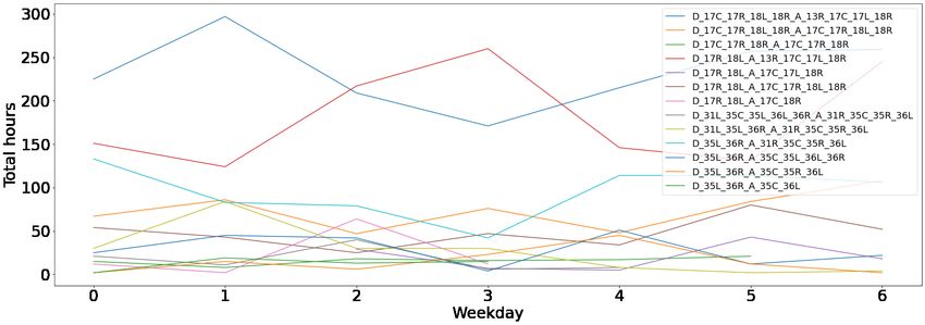
of the predictions. Configuration changes are not frequent, typically a few times a day. Having the prior configuration
value as input helps the model to learn to propagate the current configuration unless there is clear evidence in the input
features of the need of a different configuration.
 Within the multi-step forecasting approach, a variety of ML models can be used to predict the airport configuration
at each step. In this work we evaluated a Random Forest classifier, and a XGBoost classifier. The Random Forest
classifier builds multiple independent decision trees based on the features and merges them together to get a more
accurate and stable prediction [9]. Whereas the XGBoost classifier also combines decision trees, it starts the combining
process at the beginning, instead of at the end [10].

 III. Data
 Our goal was not only to develop a state of art airport configuration prediction model, but also to build a framework
to facilitate training models across many airports and deploying them in a real time system. For that reason, real time
availability was required for all input data sources, as described in this section.

A. Weather Forecast
 Weather is one of the key drivers of airport configuration. Tail winds or crosswinds can have a significant impact on
runway operations and active configuration. Inclement weather can also affect configuration and capacity, e.g. closing
of an arrival fix. In the work presented in this paper weather data is obtained from Localized Aviation MOS Program
(LAMP). The products in the LAMP system are updated hourly and are valid over a 25-hour period, and are provided
for major US airports. In this work we evaluated the following products:
 • Wind Speed, Wind Direction and Wind Gust: Wind speed and direction are important factors in determining
 airport configuration. The operational status of the runways is affected by the presence of strong crosswinds and
 tailwinds [11]. Also, wind gust, if present, can significantly affect the terminal airspace capacity.
 • Cloud Ceiling and Visibility: The cloud ceiling and the visibility at the airport influence the choice of runway
 configuration. Both runway operations, as well as capacity, are affected by low visibility conditions.
 • Temperature, Lightning probability and Precipitation: Temperature, inclement weather, presence of wet or icy
 conditions also affects the runways capacity (e.g., affecting the taxi time duration), and hence affects configuration
 utilization [12].

B. Future Arrival/Departure Counts
 The active airport configuration needs to provide enough capacity to accommodate departure and arrival flights.
Consequently, we need to estimate future traffic to predict the airport configuration. In this effort, we leverage landing
time predictions selected from physics-based landing time predictions available in FAA System Wide Information
Management (SWIM) data feeds for each flight. Following a data-driven approach, we analyzed Traffic Flow Management
(TFM) estimated time of arrivals (ETAs), Time-Based Flow Management (TBFM) ETAs and TBFM scheduled time of
arrivals (STAs) and defined a set of rules to select the most accurate ETA at the different phases of flight. For example,
TBFM ETA accuracy is poor prior to departure, being outperformed by TFM ETA. The obtained physics-based ETAs
are used to calculate future arrival counts input to our model. A detailed description of the logic can be found in
[13]. Departure counts are obtained using Traffic Flow Management System (TFMS) departure times estimate. As an
example, Fig 2 shows two weeks of arrival counts for Dallas/Fort Worth International Airport (DFW).

C. Airport Configuration
 Historical airport configuration values were obtained from Data-link Automatic Terminal Information Service
(D-ATIS) messages. The messages specify the active arrival and departure configurations over time. The airport
configuration defines our target variable and the current configuration feature.
 Due to the large number of airport configurations identified in the D-ATIS data for some airports (e.g over 90
different runway sets for DFW ), we kept only major airport configurations by removing those configurations that were
active for less than 1 % of the time. We also removed time periods with stale configurations, defined as those with no
D-ATIS updates for at least 2 hours. This typically happens at overnight hours. Accordingly, we dropped the data rows
related to the removed configurations throughout the whole time period. Fig 3 shows the DFW configurations’ total
hours per day of the week for 5 months, after applying filtering of the configurations. Out of a 90 configurations set,
only 13 configurations with their associated data were used after applying the filtering rules.

 3

Fig. 2 Arrival counts for two weeks for DFW

 Fig. 3 Configurations usage by the day of the week for filtered DFW configurations

 IV. Features
 Table 1 summarizes the features input to our ML model at each step. It includes the data described in the previous
section and the additional features defined below.

A. Time of Day
 The airport traffic changes with time of day. During the night time, the traffic will be lower than the day time. This
can lead to some configurations being more likely to be active at a certain time of day. Environmental effects, e.g. noise,
can also dictate the airport configuration at a specific time of the day. For these reasons, we included the time of day as
a feature in our model.

B. Look ahead time
 In our recursive multi-step model, we need to feed the lookahead time for the current step as a feature. This feature
helps the model to understand how the uncertainty evolves for different lookahead times and provides a more accurate
prediction.

 4

C. Airport configuration encoder
 As described in section II, the current configuration feature is only fed to the first step model as a categorical
feature and also encoded as a numerical vector. Airport runways are numbered according to compass bearings
[14]. This allow us to easily encode the current runway configuration as the average departure runway bearing,
average arrival runway bearing and total number of departure and arrival runways. For example, for the configuration
D_17R_18L_A_17C_17R_18L_18R (indicating departure runways 17R and 18L and arrival runways 17C, 17R, 18L,
and 18R), the encoder will consist of 4 fields (17.5, 2, 17.5, 4), being 17.5 the average departure runway bearing, 2
the number of active departure runways, 17.5 the average arrival runway bearing, and 4 the number of active arrival
runways respectively. The advantage of encoding the current configuration as a numeric vector is that it helps the model
to understand which configurations are similar in the encoded space and establish a notion of distance in the ML model.

 Feature Data type Description
 Time of the day Datetime Hour of the day
 Surface temperature forecast value for each step in
 Temperature Numeric
 the model look ahead window
 Wind direction forecast value in degrees for each
 Wind direction Numeric
 step in the model look ahead window
 Wind direction forecast value in degrees for each
 Wind speed Numeric
 step in the model look ahead window
 10-meter wind gust forecast value in knots for each
 Wind gust Numeric
 step in the model look ahead window
 Ceiling height categorical value in knots for each
 Cloud ceiling Numeric
 step in the model look ahead window
 Total sky cover value in knots for each step in the
 Cloud Categorical
 model look ahead window
 Visibility value for each step in the model look
 Visibility Numeric
 ahead window
 Probability of lightning value for each step in the
 Lightening Categorical
 model look ahead window
 Probability of precipitation value for each step in
 Precipitation Boolean
 the model look ahead window
 An airport configuration encoder that captures the
 Current airport Categorical,
 average runway number, along with the number of
 configuration Numeric
 active runways in each configuration
 Number of future airport arrivals for each step in
 Arrival count Numeric
 the model look ahead window
 Number of future airport departures for each step
 Departure count Numeric
 in the model look ahead window
 Look ahead time Numeric Look ahead time for current step
 Table 1 ML Model input features and Description

 V. Experimental Design and Results

A. Model Performance on 2019 data
 In this section we review the performance of the airport configuration prediction model for six selected airports:
Charlotte Douglas International Airport (CLT), DFW, John F. Kennedy International Airport(JFK), Newark Liberty
International Airport(EWR), Dallas Love Field Airport (DAL) and LaGuardia Airport (LGA) . The results in this section
were obtained for 5 months of data, August to December 2019. We selected 80% of the data for training and 20% for

 5

testing. To avoid correlation and data leakage between training and test data points, we split the data on a weekly basis,
such that the testing data contains 4 full weeks (20% of the dataset). We tested two different ML algorithms for the ML
model component in Fig. 1, Random Forest and XGBoost. The results in Fig. 4 are for XGBoost, which led to better
model performance as shown in Fig 6.
 The models for CLT and DFW were obtained for the configurations shown in Table A.1, extracted from D-ATIS
data. As previously mentioned, the configuration data was cleaned by removing rare configurations with very few data
points; i.e. we kept only configurations that were active at least 1% of the time.
 The model performance is compared with a baseline which assumes no changes in the configuration. Consequently,
the baseline propagates the current configuration up to 6 hours ahead.The model accuracy is measured as the percentage
of prediction time steps (i.e 30-minute intervals), in which the predicted configuration matches the actual configuration.
Fig. 5a shows the accuracy for the CLT model vs the baseline as a function of the planning horizon. We can see that the
baseline and model perform similarly for a short planning horizon, but for a longer planning horizon the ML model
outperforms the baseline. At 3 hours ahead, the difference between baseline and the ML model is 9%, for 6 hours ahead
the difference increases to 17%.
 A similar analysis was performed for DFW, JFK, EWR, LGA and DAL. Figs. 5b to 5f show the prediction accuracy
of the ML models vs the baseline on the testing set for these additional airports.. For DFW, the model and baseline
started performing similarly for 1 hour ahead, and then the model started to outperform the baseline by 9% 2 hours
ahead, 13% 3 hours ahead, and 31% 6 hours ahead. For JFK, EWR and DAL airports, the model performance is closer
to the baseline and the model outperforms the baseline after a longer planning horizon. For DAL airport, the model
didn’t perform better than the baseline at any point of time.
 A summary of the prediction model accuracy results for the 6 airports for 3 and 6 hours lookahead time can be found
in Figs 4a and 4b respectively. Overall, the results show that our model outperforms the baseline for most airports, but
different operating conditions at different airports affect how much performance lift the proposed model provides.
 To gain additional insights and better understand the difference in model performance across the selected airports,
we identified the most important features for each of the models. Through the evaluations done over the six airports, for
most of the airports it was noticed that the traffic (i.e, arrival and departure counts), along with the time of the day and
wind are the most important features deriving the predictions. However, for DAL airport, it was noticed that traffic
features are not within the most important features, meaning that traffic is not driving the predicted configurations, as it
is the case with the other airports. The time of the day as well as the wind features (wind direction, wind speed) are the
key features for DAL. We believe that the reason why our model was unable to perform better than the baseline for
DAL is the lack of predictive power of the traffic features, and the existence of other external factors driving the active
configuration in DAL and not included in our model. Fig A.2a, A.2b , show the most important features for DFW and
DAL airports. Given the poor performance of the model for DAL airport, we conducted some initial analysis to study
the interactions between DAL and DFW. We found that the flow in the two airports are in sync, but the configurations
within the flow seemed to be independent. Further study is needed to better understand initial findings.

 (a) 3 hours lookahead time for 2019 data (b) 6 hours lookahead time for 2019 data

 Fig. 4 Baseline vs Prediction Accuracy

 6

(a) CLT Model accuracy Vs Baseline (b) DFW Model accuracy Vs Baseline

 (c) JFK Model accuracy Vs Baseline (d) EWR Model accuracy Vs Baseline

 (e) DAL Model accuracy Vs Baseline (f) LGA Model accuracy Vs Baseline

 Fig. 5 Model Testing Prediction Accuracy vs Baseline for 6 airports -2019 data

B. Model Performance on 2020 data
 We also evaluated the performance of the airport configuration prediction model for five selected airports using
August to December 2020 data. We studied the effect of the pandemic, i.e. how the change in traffic levels can affect the
performance of the prediction model. The following subsections review the performance of the model for DFW, DAL
and North East Corridor (NEC) airports (JFK, EWR and LGA).

1. Model Performance on DFW and DAL airports
 Figs.7a,7b and Figs. A.3a, A.3b show the model prediction accuracy along with the feature importance for DFW
and DAL airports respectively. The feature importance values are calculated based on the information gain provided by
each feature when training the XGBoost trees [15]. A significant change in the feature importance for DFW for 2020

 7

Fig. 6 Random Forest Vs XGBoost model prediction accuracy for DFW airport

compared to 2019 is the large gap between the importance of the time of the day feature and the other features. This gap
shows that the best predictor is the time of day, and other relevant features, like traffic, are not playing such an important
role in 2020. DFW traffic was low in 2020 due to the pandemic, which made it harder for the model to capture the
correlation between the traffic counts and the configuration changes. For DAL, there was no significant change between
the model’s performance on 2019 vs 2020 data. The traffic counts were not relevant in either year. The time of the day
and the wind direction were the most influential features for the configuration changes in DAL. We expect the overall
model performance to improve as traffic increases in 2021.

 (a) DFW airport (b) DAL airport

 Fig. 7 Model accuracy Vs Baseline for 2020 Data

2. Model Performance NEC airports
 Similarly, we evaluated the performance of the prediction model for NEC airports. Figs. 8a to 8c, and Figs. A.4a
to A.4c show the model prediction accuracy along with the feature importance for JFK, EWR and LGA airports
respectively. As with DFW airport, it was clear that JFK and EWR traffic was also affected by the pandemic, which
lead to the decrease in the performance of the model. For LGA airport, the traffic features were not within the most
important features in either 2019 and 2020 data, meaning that traffic is not driving the predicted configuration. Thus,
the performance of the model for LGA for both years was nearly the same.
 We also performed an analysis in order to study how changes in the configuration in one of the airports can
affect others, and the main factors influencing the chosen airport configuration. The goal was to better understand
interactions among the NEC airports, and how the insights could be used to improve the developed prediction models
for these and other airports in the New York area. Figs.9a, 9b show the correlation matrices for JFK, EWR and LGA

 8

(a) JFK airport (b) EWR airport

 (c) LGA airport

 Fig. 8 NEC Model accuracy Vs Baseline for 2020 Data

configurations. The dependency matrices show the configuration usage percentages for each airport and how the
configurations for different airports overlap with each other. The configuration information shown in the figures do not
contain all active runways, but the unique values of the compass bearing of the active runways, e.g. JFK configuration
D_22R_A_22L shown as 22. This representation provides a more clear notion of flow, and aggregates some of the
underlying configurations. As expected, the results show that wind direction is an important factor driving airport
configuration. It was found that LGA was mostly using runways 13 and 22 when JFK was using runway 22. In addition,
the use of runway 22 at EWR is frequently corresponding to the use of 22 at JFK. These configurations are used for
southern wind conditions. Similarly, the use of the runway 4 at EWR corresponds to the use of runways 31 and 4 for JFK,
which would be used for northern winds. We also reviewed the sequence of configuration changes to better understand
if any of the airports is driving configuration changes at others airports. However, the results were inconclusive, we did
not find any strong relationships for our current data set. These are preliminary results, more study will be conducted to
better understand interactions in future steps.

 VI. Conclusion
 In this paper, a multi-step machine learning approach is proposed for predicting airport configuration. The approach
guarantees stability of the predicted configuration by taking as input the configuration predicted at the previous time
step.The performance of the proposed model was tested and validated on six major US airports, spanning data from
both 2019 and 2020. We compared the model’s performance for both years to evaluate how the change in traffic levels
in 2020 due to the pandemic affects the performance of the prediction model. It was clear that traffic counts, time
of the day, and wind speed and direction features were the most important features affecting airport configurations
changes. The proposed model performed better on 2019 data than on 2020, due to the decrease in the effect of traffic
features because of the pandemic. The results presented in this paper demonstrate the value of the proposed approach.
The proposed baseline was consistently outperformed as the prediction horizon increases. An important aspect of the
proposed framework is the real time nature of the data, and the implementation using state of art machine learning

 9

(a) JFK-LGA configurations correlation matrix (b) JFK-EWR configurations correlation matrix

 Fig. 9 NY airports configuration correlation matrix

practices and tools to facilitate experimentation and deployment. Consequently, the proposed model can be integrated in
a real time system and deployed for many airports with a low level of effort
 As next steps, we plan on testing our model on 2021 data to evaluate and compare its performance against 2019 and
2020 data. For NEC airports, we plan to study in detail the NEC area airports by designing a combined model that uses
the input features from the NY airports and predicts a combined airport configuration.

 10

A. Appendix

Airport Configurations
 D_18C_18L_A_18C_18L
 D_18C_18L_A_18C_18L_18R
 D_18C_A_18C
 D_18C_A_18C_18R
CLT
 D_36C_36R_A_36C_36L_36R
 D_36C_36R_A_36C_36R
 D_36C_A_36C
 D_36C_A_36C_36L
 D_17C_17R_18L_18R_A_13R_17C_17L_18R
 D_17C_17R_18L_18R_A_17C_17R_18L_18R
 D_17C_17R_18R_A_17C_17R_18R
 D_17R_18L_A_13R_17C_17L_18R
 D_17R_18L_A_17C_17L_18R
 D_17R_18L_A_17C_17R_18L_18R
DFW
 D_31L_35C_35L_36L_36R_A_31R_35C_35R_36L
 D_31L_35L_36R_A_31R_35C_35R_36L
 D_35L_36R_A_31R_35C_35R_36L
 D_35L_36R_A_35C_35L_36L_36R
 D_35L_36R_A_35C_35R_36L
 D_35L_36R_A_35C_36L
 D_13R_A_13R
 D_13L_13R_A_13L_13R
 D_31L_31R_A_31L_31R
DAL
 D_13L_A_13L
 D_31L_A_31L
 D_31R_A_31R
 D_22R_A_22L
 D_22R_A_22L_22R
 D_4L_A_4L_4R
JFK D_13R_A_13L
 D_31L_A_31L_31R
 D_4L_A_4L
 D_4L_A_4R
 D_13_A_13
 D_13_A_22
 D_31_A_22
LGA D_13_A_4
 D_4_A_31
 D_31_A_4
 D_4_A_4
 D_22R_A_22L
 D_22R_A_22R
 D_4L_A_4R
EWR
 D_22L_A_22L
 D_4L_A_4L
 D_4R_A_4R
 Table A.1 D-ATIS Filtered Airport configurations

 11

(a) DFW Features Importance (b) DAL Model Features importance

 Fig. A.2 DFW and DAL feature importance for 2019 Data

 (b) DAL airport
 (a) DFW airport

 Fig. A.3 Feature Importance for 2020 Data

 12

(a) JFK airport (b) EWR airport

 (c) LGA airport

 Fig. A.4 NEC airports Feature Importance for 2020 Data

 Acknowledgments
 The authors gratefully acknowledge funding for this work from the National Aeronautics and Space Administration
(NASA) as part of the Airspace Technology Demonstration 2 (ATD-2) project.

 References
 [1] Provan, C. A., and Atkins, S. C., Optimization models for strategic runway configuration management under weather uncertainty,
 2010. https://doi.org/10.2514/6.2010-9149, URL https://arc.aiaa.org/doi/abs/10.2514/6.2010-9149.
 [2] Bertsimas, D., Frankovich, M., and Odoni, A., “Optimal Selection of Airport Runway Configurations,” Oper. Res., Vol. 59,
 No. 6, 2011, p. 1407–1419. https://doi.org/10.1287/opre.1110.0956, URL https://doi.org/10.1287/opre.1110.0956.
 [3] Hesselink, H. H., and Nibourg, J., “Probabilistic 2-Day Forecast of Runway Use,” Proceedings of Ninth USA/Europe Air Traffic
 Management Research and Development Seminar (ATM2011), 2011.
 [4] Houston, S., and Murphy, D., “Predicting runway configurations at airports,” Transportation Research Board (TRB) Annual
 Meeting, 2012, pp. 12–3682.
 [5] Avery, J., and Balakrishnan, H., “Data-Driven Modeling and Prediction of the Process for Selecting Runway Configurations,”
 Transportation Research Record, Vol. 2600, No. 1, 2016, pp. 1–11. https://doi.org/10.3141/2600-01, URL https://doi.org/10.
 3141/2600-01.
 [6] Ahmed, M. S., Alam, S., and Barlow, M., “A Multi-Layer Artificial Neural Network Approach for Runway Configuration
 Prediction,” Proceedings of the 8th International Conference on Research in Air Transportation (ICRAT 2018), Castelldefels,
 Spain, 2018.

 13

[7] Jones, J. C., DeLaura, R., Pawlak, M. L., Troxel, S., and Underhill, N., “Predicting & Quantifying Risk in Airport Capacity
 Profile Selection for Air Traffic Management,” Proceedings of 14th USA/Europe Air Traffic Management Research and
 Development Seminar (ATM2017), Seattle, USA, 2017.

 [8] Cheng, H., Tan, P.-N., Gao, J., and Scripps, J., “Multistep-Ahead Time Series Prediction,” Advances in Knowledge Discovery
 and Data Mining, edited by W.-K. Ng, M. Kitsuregawa, J. Li, and K. Chang, Springer Berlin Heidelberg, Berlin, Heidelberg,
 2006, pp. 765–774.

 [9] Breiman, L., “Random Forests,” Machine Learning, Vol. 45, 2001, pp. 5–32. https://doi.org/10.1023/A:1010933404324, URL
 https://doi.org/10.1023/A:1010933404324.

[10] Chen, T., and Guestrin, C., “XGBoost,” Proceedings of the 22nd ACM SIGKDD International Conference on Knowledge
 Discovery and Data Mining, 2016. https://doi.org/10.1145/2939672.2939785, URL http://dx.doi.org/10.1145/2939672.2939785.

[11] Kicinger, R., Chen, J.-T., Steiner, M., and Pinto, J., “Airport Capacity Prediction with Explicit Consideration of Weather
 Forecast Uncertainty,” Journal of Air Transportation, Vol. 24, 2016, pp. 18–28. https://doi.org/10.2514/1.D0017.

[12] Hunter, G., “Probabilistic forecasting of airport capacity,” 2010, pp. 2.A.3–1. https://doi.org/10.1109/DASC.2010.5655497.

[13] Wesely, D., Churchill, A., Slough, J., and Coupe, W. J., “A Machine Learning Approach to Predict Aircraft Landing Times
 using Mediated Predictions from Existing Systems,” Submitted to AIAA AVIATION Forum, Washington, DC, USA, 2021.

[14] “Airport Runway Names Shift with Magnetic Field,” 2017. URL https://www.ncei.noaa.gov/news/airport-runway-names-shift-
 magnetic-field.

[15] “XGBoost: A Scalable Tree Boosting System,” Proceedings of the 22nd ACM SIGKDD International Conference on
 Knowledge Discovery and Data Mining, Association for Computing Machinery, New York, NY, USA, 2016, p. 785–794.
 https://doi.org/10.1145/2939672.2939785, URL https://doi.org/10.1145/2939672.2939785.

 14