Torchvision And Random Tensors - Purdue Engineering
←
→
Page content transcription
If your browser does not render page correctly, please read the page content below
Torchvision And Random Tensors

                    Lecture Notes on Deep Learning

                    Avi Kak and Charles Bouman

                             Purdue University

                    Sunday 3rd January, 2021     22:54

Purdue University                                        1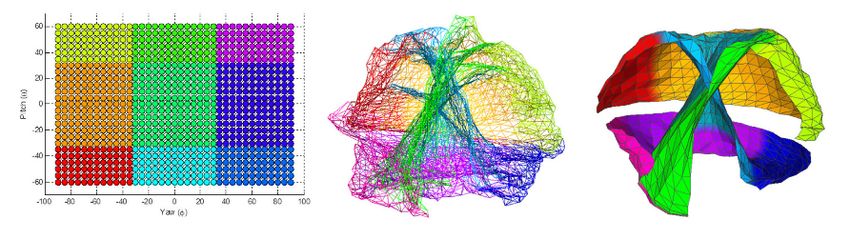
Preamble

Deep learning owes its success (as measured by performance evaluation over
datasets consisting of millions of images) only partly to the architectures of the
networks.

The other reason for that success is data augmentation.

Consider an autonomous vehicle of the future that must learn to recognize the
stop signs with almost no error. As explained in this presentation, the learning
required for this is not as simple as it may sound. As the vehicle approaches a
stop sign, how it shows up in the camera image will undergo significant
transformations.

So how can the neural network used by the vehicle be trained so that it would
work well despite these transformations? The answer: Through data
augmentation of the sort that is presented here.

 Purdue University                                                                   2
Preamble

Given a set of training images, you can use the functionality of
torchvision.transforms to augment your training data in order to address the
challenge described above.

Given its importance, the primary goal of this lecture is to develop a working level
familiarity with the different classes of Torchvision.

In addition to serving as an introduction to Torchvision, a second goal of this
lecture is to make you familiar with PyTorch’s functionality for generating random
data. In particular, I’ll focus on how to create tensors with random data drawn
from different distributions.

The syntax examples I’ll use with random tensors are also meant to make you
familiar with the tensor shapes that are expected by neural networks at their
inputs, and with the estimation of different types of histograms for those tensors.
 Purdue University                                                                3
Outline

1    Transformations for Data Augmentation               5

2    Illumination Angle Dependence of the Camera Image   16

3    Greyscale and Color Transformations                 18

4    The Compose Class                                   28

5    Torchvision for Image Processing                    32

6    Constructing Random Tensors with PyTorch            36

7    Working with Image-Like Random Tensors              45

    Purdue University                                    4
Transformations for Data Augmentation
Outline
1 Transformations for Data Augmentation 5
2 Illumination Angle Dependence of the Camera Image 16
3 Greyscale and Color Transformations 18
4 The Compose Class 28
5 Torchvision for Image Processing 32
6 Constructing Random Tensors with PyTorch 36
7 Working with Image-Like Random Tensors 45
Purdue University 5Transformations for Data Augmentation
Making the Case for Transformations for
Augmenting the Training Data
Let’s say you want to create a neural-network (NN) based stop sign
detector for an autonomous vehicle of the future. Here are the challenges
for your neural network:
The scale issue: A vehicle approaching an intersection would see the stop sign at different scales;
Illumination issues: The NN will have to work despite large variations in the image caused by illumination effects that would
depend on the weather conditions and the time of the day and, when the sun is up, on the sun angle;
Viewpoint effects: As the vehicle gets closer to the intersection, its view of the stop sign will be increasingly non-orthogonal.
The off-perpendicular views of the stop sign will first suffer from affine distortion and then from
projective distortion. The wider a road, the larger these distortions. [Isn’t it interesting that human
drivers do not even notice such distortions — because of our expectation driven perception of the reality.]
While creating this slide, I was reminded of our own work on
neural-network based indoor mobile robot navigation. This work is now
25-years old. Did you know that Purdue-RVL is considered to be a pioneer
in indoor mobile robot navigation research? Here is a link to that old work:
https://engineering.purdue.edu/RVL/Publications/Meng93Mobile.pdf
Purdue University 6Transformations for Data Augmentation
Augmenting the Training Data
Deep Learning based frameworks commonly use data augmentation to
cope with the sort of challenges listed on the previous slide.
Data augmentation means that in addition to using the images that
you have actually collected, you also create transformed versions of
the images, with the transformations corresponding to the various
effects mentioned on the previous slide.
In the next several slides, I’ll talk about what these transformations
look like and what functions in torchvision.transforms can be
invoked for the transformations.
Purdue University 7Transformations for Data Augmentation
Homographies for Image Transformations
Image transformations in general are nonlinear. If you point a camera on a
picture mounted on a wall, because of lens optics in the camera, the
relationship between the coordinates of the points in the picture and the
coordinates of the corresponding pixels in the camera image is nonlinear.
Nonlinear transformations are computationally expensive.
Fortunately, through the magic of homogeneous coordinates, these
transformations can be expressed as linear relationships in the form of
matrix-vector products.
[NOTE: Did you know that much of the power that modern engineering derives from the use of homogeneous coordinates
is based on the work of Shreeram Abhyankar, a great mathematician from Purdue? He passed away in 2012 but his work on
algebraic geometry continues to power all kinds of modern applications ranging from Google maps to robotics. ]
Purdue University 8Transformations for Data Augmentation
Homogeneous Coordinates
Consider a camera taking a photo of a wall mounted picture. What happens
to the relationship between the point coordinates on the wall and the pixel
coordinates as you view the picture from different angles?
Let (x, y ) represent the coordinates of a point in a wall mounted picture.
Let (x 0 , y 0 ) represent the coordinates of the pixel in the camera image that
corresponds to the point (x, y ) on the wall.
In general, the pixel coordinates (x 0 , y 0 ) depend nonlinearly on the point
coordinates (x, y ). Even when the imaging plane in the camera is parallel to
the wall, this relationship involves a division by the distance between the two
planes. And when the camera optic axis is at an angle with respect to the
wall normal, you have a more complex relationship between the two planes.
Purdue University 9Transformations for Data Augmentation
Homogeneous Coordinates (contd.)
We use homogeneous coordinates (HC) to simplify the relationship
between the two planes.
In HC, we bring into play one more dimension and represent the same
point with three coordinates (x1 , x2 , x3 ) where
x1
x= x3
x2
y= x3
A 3 × 3 homography is a mapping from the wall plane represented by
the coordinates (x, y ) to the imaging plane represented by the
coordinates (x 0 , y 0 ). It is given by the matrix shown below:
" x0 # " h h12 h13 #" x1 #
1 11
0
x2 = h21 h22 h23 x2
x30 h31 h32 h33 x3
The above relationship is expressed more compactly as x0 = Hx
where H is the homography.
Purdue University 10Transformations for Data Augmentation
Homography and the Distance Between the
Camera and the Object
The homography matrix H acquires a simpler form when our
autonomous vehicle of the future is at some distance from the stop
sign. This simpler form is known as the Affine Homography.
However, as the vehicle gets closer and closer to the stop sign, the
relationship between the plane of the stop sign and camera imaging
plane will change from Affine to Projective.
The homography shown on the previous slide is the Projective
homography. The next slide talks about the Affine Homography.
A Projective Homography always maps straight lines into straight
lines.
Purdue University 11Transformations for Data Augmentation
Affine Homography — A Special Cases of the 3 × 3
Homography
As mentioned on the previous slide, when the vehicle is at some
distance from a stop sign, the relationship between the plane of the
stop sign and the camera image plane is likely to be what is known as
the affine homography:
" x0 # " a a12 t1 #" x1 #
1 11
0
x2 = a21 a22 t2 x2
x30 0 0 1 x3
An affine homography always maps straight lines in a scene into
straight lines in the image. Additionally, the parallel lines remain
parallel.
Purdue University 12Transformations for Data Augmentation
Affine vs. Projective Distortions
Affine
Projective
Figure: Affine: Straight lines remain straight and parallel lines remain parallel.
Projective: Straight lines remain straight.
Purdue University 13Transformations for Data Augmentation
Affine Transformation Functionality in
torchvision.transforms
class
torchvision.transforms.RandomAffine(degrees, translate=None, scale=None, shear=None, resample=False, fillcolor=
Random affine transformation of the image keeping center invariant
Parameters
degrees (sequence or python:float or python:int) { Range of degrees to select from.
If degrees is a number instead of sequence like (min, max), the range of
degrees will be (-degrees, +degrees). Set to 0 to deactivate rotations.
translate (tuple, optional) { tuple of maximum absolute fraction for horizontal and vertical translations.
For example translate=(a, b), then horizontal shift is randomly sampled in the range
-img_width * a < dx < img_width * a and vertical shift is randomly sampled in the range
-img_height * b < dy < img_height * b. Will not translate by default.
scale (tuple, optional) { scaling factor interval, e.g (a, b), then scale is randomly sampled
from the range aTransformations for Data Augmentation
Projective Transformation Functionality in
torchvision.transforms
torchvision.transforms.functional.perspective(img, startpoints, endpoints, interpolation=3)
Perform perspective transform of the given PIL Image.
Parameters
img (PIL Image) { Image to be transformed.
startpoints { List containing [top-left, top-right, bottom-right, bottom-left] of the orignal image
endpoints { List containing [top-left, top-right, bottom-right, bottom-left] of the transformed image
interpolation { Default- Image.BICUBIC
Purdue University 15Illumination Angle Dependence of the Camera Image
Outline
1 Transformations for Data Augmentation 5
2 Illumination Angle Dependence of the Camera Image 16
3 Greyscale and Color Transformations 18
4 The Compose Class 28
5 Torchvision for Image Processing 32
6 Constructing Random Tensors with PyTorch 36
7 Working with Image-Like Random Tensors 45
Purdue University 16Illumination Angle Dependence of the Camera Image
Illumination Angle Effects
While we understand quite well how a camera of a planar object is likely to
change as the camera moves closer to the plane of the object or farther
away from it, the dependence of the image on different kinds of illumination
properties is much more complex and data augmentation with respect to
these effects still not a part of DL frameworks.
Figure: The face image data for three different human subjects resides on the manifolds shown. The depiction is
based on the first three eigenvectors of the data.
This figure shown above is from our publication:
https://engineering.purdue.edu/RVL/Publications/FaceRecognitionUnconstrainedPurdueRVL.pdf
An application may also require data augmentation with respect to the
spectrum of illumination. Regarding how the color content in an image
changes with different illumination spectra, see http://docs.lib.purdue.edu/ecetr/8
Purdue University 17Greyscale and Color Transformations
Outline
1 Transformations for Data Augmentation 5
2 Illumination Angle Dependence of the Camera Image 16
3 Greyscale and Color Transformations 18
4 The Compose Class 28
5 Torchvision for Image Processing 32
6 Constructing Random Tensors with PyTorch 36
7 Working with Image-Like Random Tensors 45
Purdue University 18Greyscale and Color Transformations
Greyscale and Color Transformations
An image is always an array of pixels. In a B&W image, each pixel is
represented by an 8-bit integer. What that means is that the grayscale
value at each pixel will be an integer value between 0 and 127.
On the other hand, a pixel in a color image typically has three values
associated with it, each an integer between 0 and 127. These three
values stand for the three color channels.
Frequently, the purpose of grayscale and color transformation is to
normalize the values so that they possess a specific mean (most
frequently zero), a specific range (more frequently -1.0 to 1.0) and a
specific standard deviation (more frequently 0.5).
Purdue University 19Greyscale and Color Transformations
Grayscale and Color Normalization in
torchvision.transforms
class
torchvision.transforms.Normalize(mean, std, inplace=False)
Normalize a tensor image with mean and standard deviation. Given mean: (M1,...,Mn) and
std: (S1,..,Sn) for n channels, this transform will normalize each channel of the
input torch.*Tensor i.e. input[channel] = (input[channel] - mean[channel]) / std[channel]
Parameters
mean (sequence) { Sequence of means for each channel.
std (sequence) { Sequence of standard deviations for each channel.
inplace (bool,optional) { Bool to make this operation in-place.
Purdue University 20Greyscale and Color Transformations
Image Normalization
Note that when transforming the integer representation in a PIL image into
a tensor, all the channel values will be converted from [0,255] ints to [0,1]
floats. It is on such a tensor that you would call
transforms.Normalize((mean, mean, mean), (std, std, std))])
The call shown above is used most commonly with the following values for
the parameters:
transforms.Normalize((0.5, 0.5, 0.5), (0.5, 0.5, 0.5))])
These parameter values convert each channel values to the (-1,1) range of
floats. The normalization of the values in each channel is carried out using
the formula:
pixel_val = (pixel_val - mean) / std
The parameters (mean, std) are passed as (0.5, 0.5) in the call shown
above. This will normalize the image in the range [-1,1]. For example, the
minimum value 0 will be converted to (0-0.5)/0.5=-1, the maximum value
of 1 will be converted to (1-0.5)/0.5=1.
In order to take the image back to the PIL form, you would first need to
change
Purdue the range
University back to [0,1] by pixel val = ((pixel val ∗ std) + mean) 21Greyscale and Color Transformations
Transforming the Color Space
Most commonly, the images are based on the RGB color channels.
However, that is not always the best strategy.
Sometimes, the discriminations you want to carry out are better
implemented in other color spaces such as HSI/V/L and L*a*b.
Purdue University 22Greyscale and Color Transformations
Does Torchvision Contain the Transforms for
Different Color Spaces
The answer is: No.
However, you can use the PIL’s convert() function for converting an image
from one color space to another. For example, if im is a PIL image in RGB
and you want to convert it into the HSV color space, you would call
x.convert(’HSV’).
If you want this color-space transformation, you would need to define your
color-space transformer class as:
def convert_to_hsv(x):
return x.convert("HSV")
But note that “x” has to be a PIL Image object. You can then use
the Lambda class in torchvision.transforms to create your own
transform class that will be treated like the native transform classes.
This you can do by defining:
my_color_xform = torchvision.transforms.Lambda(lambda x: convert_to_hsv(x))
Purdue University 23Greyscale and Color Transformations
Transforming the Color Space (contd.)
Subsequently, you would want to embed the my color xform in a
randomizer so that it changes the images in each batch in each
epoch. That way, the same image would be seen through different
color spaces in different epochs.
This can easily be done by calling on the RandomApply class as
follows:
random_colour_transform = torchvision.transforms.RandomApply([colour_transform], p)
where the second argument, p, is set to the probability with which
you would want your color transformer to be invoked. Its default
value is 0.5.
Purdue University 24Greyscale and Color Transformations
Transforming the Color Space (contd.)
Here is another data augmentation function from
torchvision.transforms that can be used to randomly change the
brightness, contrast, saturation, and hue levels in an image:
class
torchvision.transforms.ColorJitter(brightness=0, contrast=0, saturation=0, hue=0)
Randomly change the brightness, contrast and saturation of an image.
Parameters
brightness (python:float or tuple of python:float (min, max)) { How much to jitter
brightness. brightness_factor is chosen uniformly from [max(0, 1 - brightness),
1 + brightness] or the given [min, max]. Should be non negative numbers.
contrast (python:float or tuple of python:float (min, max)) { How much to jitter
contrast. contrast_factor is chosen uniformly from [max(0, 1 - contrast), 1 + contrast]
or the given [min, max]. Should be non negative numbers.
saturation (python:float or tuple of python:float (min, max)) { How much to jitter saturation.
saturation_factor is chosen uniformly from [max(0, 1 - saturation), 1 + saturation]
or the given [min, max]. Should be non negative numbers.
hue (python:float or tuple of python:float (min, max)) { How much to jitter hue.
hue_factor is chosen uniformly from [-hue, hue] or the given [min, max].
Should have 0Greyscale and Color Transformations
Converting a Tensor Back to a PIL Image
Say that the output of a calculation is a tensor that represents an image.
At some point you would want to display the tensor. For that, you have to
first convert the tensor to a PIL image. This can be done by calling on the
torchvision.transforms.ToPILImage() method presented here:
class
torchvision.transforms.ToPILImage(mode=None)
Convert a tensor or an ndarray to PIL Image.
Converts a torch.*Tensor of shape C x H x W or a numpy ndarray of shape H x W x C to a PIL Image while pres
Parameters
mode (PIL.Image mode) {
color space and pixel depth of input data (optional). If mode is None (default) there are some assumpti
If the input has 4 channels, the mode is assumed to be RGBA.
If the input has 3 channels, the mode is assumed to be RGB.
If the input has 2 channels, the mode is assumed to be LA.
If the input has 1 channel, the mode is determined by the data type (i.e int, float, short).
Purdue University 26Greyscale and Color Transformations
If Color is Important, Why Not Texture?
Yes, there is much information in texture also, although most
published papers on CNN based image recognition do not mention
texture at all.
See the following paper that talks about the role texture has played in
the results that researchers have obtained with CNNs:
https://arxiv.org/pdf/1811.12231.pdf
You might also want to see the following tutorial by me on color and
texture: https://engineering.purdue.edu/kak/Tutorials/TextureAndColor.pdf
Purdue University 27The Compose Class
Outline
1 Transformations for Data Augmentation 5
2 Illumination Angle Dependence of the Camera Image 16
3 Greyscale and Color Transformations 18
4 The Compose Class 28
5 Torchvision for Image Processing 32
6 Constructing Random Tensors with PyTorch 36
7 Working with Image-Like Random Tensors 45
Purdue University 28The Compose Class
Using the Compose Class as a Container of
Transformations
torchvision.transforms provides you with a convenient class called
Compose that serves as a “container” for all the transformations you want
to apply to your images before they are fed into a neural network.
Consider the following three different invocations of Compose:
resize_xform = tvt.Compose( [ tvt.Resize((64,64)) ] ) ## (A)
gray_and_resize = tvt.Compose( [tvt.Grayscale(num_output_channels = 1),
tvt.Resize((64,64)) ] ) ## (B)
gray_resize_normalize = tvt.Compose( [tvt.Grayscale(num_output_channels = 1),
tvt.Resize((64,64)),
tvt.ToTensor(),
tvt.Normalize(mean=[0.5], std=[0.5]),
tvt.ToPILImage() ] ) ## (C)
What you see on the LHS for each of the three cases is an instance of the
Compose class — although a callable instance.
Purdue University 29The Compose Class
Applying the “Composed” Transformations to the
Images
The torchvision.transforms functionally is designed to work on PIL
(Python Image Library) images. So you must first open your disk-stored
image file as follows:
im_pil = Image.open(image_file)
Subsequently, you could invoke any of the following commands:
img = resize_xform( im_pil )
img = gray_and_resize( im_pil )
img = gray_resize_normalize( im_pil )
depending on what it is that you want to do to the image.
Purdue University 30The Compose Class
Converting a PIL Image Into a Tensor
Given a PIL image, img, you can convert into into a [0,1.0]-range tensor
by the following transformation:
img_tensor = tvt.Compose([tvt.ToTensor()])
img_data = img_tensor(img)
Note again that we must first construct a callable instance of Compose
and then invoke it on the image that needs to be converted to a tensor.
Now we can apply, say, a comparison operator to it as follows:
img_data = img_data > 0.5
which returns a tensor of booleans (which, for obvious reasons, cannot be
displayed directly in the form of an image). To create an image from the
booleans, we can use the following ploy:
img_data = img_data.float()
to_image_xform = tvt.Compose([tvt.ToPILImage()])
img = to_image_xform(img_data)
You can see this code implemented in the function
graying resizing binarizing() of my RegionProposalGenerator module.
Purdue University 31Torchvision for Image Processing
Outline
1 Transformations for Data Augmentation 5
2 Illumination Angle Dependence of the Camera Image 16
3 Greyscale and Color Transformations 18
4 The Compose Class 28
5 Torchvision for Image Processing 32
6 Constructing Random Tensors with PyTorch 36
7 Working with Image-Like Random Tensors 45
Purdue University 32Torchvision for Image Processing
Accessing the Color Channels
Shown below are examples of statements you’d need to make if you want
to access the individual color channels in an image. I have lifted these
statements from the RegionProposalGenerator module that, by the way,
you can download from
https://pypi.org/project/RegionProposalGenerator/1.0.4/
im_pil = Image.open(image_file)
image_to_tensor_converter = tvt.ToTensor() ## for conversion to [0,1] range
image_as_tensor = image_to_tensor_converter(im_pil)
print(type(image_as_tensor)) ##
print(image_as_tensor.type()) ##
print( image_as_tensor.shape) ) ## (3, 366, 320)
channel_image = image_as_tensor[n]
gray_tensor = 0.4 * image_as_tensor[0] + 0.4 * image_as_tensor[1] + 0.2 * image_as_tensor[2]
Purdue University 33Torchvision for Image Processing
Working with Color Spaces
An example that shows the kinds of calls you’d need to make for color
space transformation, etc.
im_pil = Image.open(image_file)
hsv_image = im_pil.convert(’HSV’)
hsv_arr = np.asarray(hsv_image)
np.save("hsv_arr.npy", hsv_arr)
image_to_tensor_converter = tvt.ToTensor()
hsv_image_as_tensor = image_to_tensor_converter( hsv_image )
This code is implemented in the function
working with hsv color space of my RegionProposalGenerator
class.
Purdue University 34Torchvision for Image Processing
Histogramming an Image
An example that shows the kinds of calls you’d need to make for
histogramming the image data:
im_pil = Image.open(image_file)
image_to_tensor_converter = tvt.ToTensor()
color_image_as_tensor = image_to_tensor_converter( im_pil )
r_tensor = color_image_as_tensor[0]
g_tensor = color_image_as_tensor[1]
b_tensor = color_image_as_tensor[2]
hist_r = torch.histc(r_tensor, bins = 10, min = 0.0, max = 1.0)
hist_g = torch.histc(g_tensor, bins = 10, min = 0.0, max = 1.0)
hist_b = torch.histc(b_tensor, bins = 10, min = 0.0, max = 1.0)
### Normalizing the channel based hists so that the bin counts in each sum to 1.
hist_r = hist_r.div(hist_r.sum())
hist_g = hist_g.div(hist_g.sum())
hist_b = hist_b.div(hist_b.sum())
See this code implemented in the function histogramming the image() of
my RegionProposalGenerator module.
Purdue University 35Constructing Random Tensors with PyTorch
Outline
1 Transformations for Data Augmentation 5
2 Illumination Angle Dependence of the Camera Image 16
3 Greyscale and Color Transformations 18
4 The Compose Class 28
5 Torchvision for Image Processing 32
6 Constructing Random Tensors with PyTorch 36
7 Working with Image-Like Random Tensors 45
Purdue University 36Constructing Random Tensors with PyTorch
Constructing Random Tensors
As already alluded to earlier in this lecture, training data
augmentation by randomizing various aspects of the available data
plays a large role in deep learning. And, as you will see in later
lectures, you also need random number generators for creating
“artificial” training and testing datasets for neural networks.
In this section, though, my goal is merely to make you familiar with
the functionality that PyTorch provides for creating random tensors.
Here is a link to the documentation page where you will find listed all
of PyTorch’s functions that you can call for creating tensors with
random data based on different probability distributions ((unform,
normal, bernoulli, multinomial, and poisson):
https://https://pytorch.org/docs/stable/torch.html#random-sampling
At the above link, you will also see functions whose names end in the
substring ” like”. These can be used to create a tensor whose shape
corresponds to that of an existing tensor but whose content is drawn
Purdue University
from a random process. 37Constructing Random Tensors with PyTorch
Constructing Random Tensors (Contd.)
In what follows, I’ll focus on just three of the functions listed at the
link on the previous slide that I find myself using all the time:
torch.randint() for uniformly distributed integer data in a tensor,
torch.rand() for filling a tensor with uniformly distributed floating
point values in the half-open interval [0,1), and
torch.randn() for filling a tensor with normally distributed
floating-point numbers with mean 0.0 and variance 1.0.
In line with what was mentioned on the previous slide, you can also
call functions with names like torch.randint like(),
torch.rand like(), and torch.randn like() for creating duplicates
of previously defined tensors that you now want to fill with random
data.
Shown on the next slide is the basic syntax for calling
torch.randint().
Purdue University 38Constructing Random Tensors with PyTorch
Constructing a Random Tensor with
torch.randint()
What is shown below is how torch.randint() is typically called. The
function outputs integers that are uniformly distributed between the
first arg value and the second arg value minus one. For the call shown
below, the output integer values will be between 0 and 15, both ends
inclusive. The third arg is a tuple that specifies the shape of the
output tensor. The call shown below says that the tensor returned by
the call has a single axis of dimension 30.
out_tensor = torch.randint(0,16,(30,))
print(out_tensor)
# tensor([12, 15, 5, 0, 3, 11, 3, 7, 9, 3, 5, 2, 4, 7, 6, 8,
# 8, 12, 10, 1, 6, 7, 7, 14, 8, 1, 5, 9, 13, 8])
print(out_tensor.dtype) # torch.int64
print(out_tensor.type()) # torch.LongTensor
Note the difference in the answers returned by calling dtype on the
tensor and doing the same with type(). The former returns the data
type of the elements in the tensor and the latter the type of the
Purdue University
tensor itself. 39Constructing Random Tensors with PyTorch
Using torch.randint() (Contd.)
Pay particular attention to the third argument in the call to
torch.randint(). As mentioned earlier, that argument is set to a
tuple that is the shape of the tensor you want torch.randint() to
return. In the call shown, I have set that to “(30,)”.
You might think that I would get the same answer as shown on the
previous slide if I changed the 3rd argument to “(30,0)”. But, what
may seem strange at first sight, here is what the code fragment
shown on the previous slide returns with “(30,0)” for the 3rd arg:
tensor([], size=(30, 0), dtype=torch.int64)
torch.int64
torch.LongTensor
As you can see, you get an empty tensor. WHY? [HINT: Using the analogies of
“vectors” and “matrices”, a vector is NOT a matrix with its row dimension set to 0. Neither is a vector a matrix with
its row dimension set to 1. For the former, setting the dimension to 0 is nonsensical — except, perhaps, for an empty
object, and, for the latter, when you set the row dimension equal to 1, you end up with a data object that requires two
pairs of square brackets to visualize it. A vector should be displayable with a single pair of square brackets that delimit
the data. Roughly the same thing happens with numpy arrays if you make the call numpy.arange(30).reshape(30,0),
except that now numpy throws an exception saying “cannot reshape array of size 30 into shape (30,0).]
Purdue University 40Constructing Random Tensors with PyTorch
Using torch.randint() (Contd.)
If you wanted to convert on the fly the data elements of the tensor
returned by torch.randint() so that they are of type torch.float, a
32-bit floating-point datatype, the following call would do that:
out_tensor = torch.randint(0,16,(30,)).float()
print(out_tensor)
# tensor([ 9., 4., 3., 0., 3., 5., 14., 15., 15., 0., 2., 3., 8., 1.,
# 3., 13., 3., 3., 14., 7., 0., 1., 9., 9., 15., 0., 15., 10.,
# 4., 7.])
print(out_tensor.dtype) # torch.float32
print(out_tensor.type()) # torch.FloatTensor
The following call shows you can create a tensor in a CPU and then
transfer it to the GPU while setting its requires grad attribute to
true.
out_tensor = torch.randint(0,16,(30,)).float().requires_grad_(True).cuda()
print(out_tensor)
# tensor([ 3., 14., 11., 2., 7., 12., 2., 0., 0., 4., 5., 5., 6., 8.,
# 4., 1., 15., 4., 9., 10., 10., 15., 8., 1., 1., 7., 9., 9.,
# 3., 6.], device=’cuda:0’, grad_fn=)
print(out_tensor.dtype) # torch.float32
print(out_tensor.type()) # torch.cuda.FloatTensor
Purdue University 41Constructing Random Tensors with PyTorch
Using torch.randint() (Contd.)
In the second example on the previous slide, note how the tensor type
changed from torch.FloatTensor to torch.cuda.FloatTensor. Such
a tensor can only reside in the GPU memory.
It is important to keep in mind that PyTorch makes a distinction
between the CPU based tensors and GPU based tensors. A GPU
based tensor comes into existence when a CPU based tensor is moved
into the GPU memory by invoking cuda() as was shown above.
The following call makes a GPU tensor directly. We now call
torch.randint() with a specific argument for the parameter device:
device = torch.device(’cuda’if torch.cuda.is_available() else ’cpu’)
out_tensor = torch.randint(0,16,(30,), dtype=torch.float, device=device, requires_grad=True)
print(out_tensor)
# tensor([ 5., 1., 7., 12., 9., 12., 7., 13., 2., 9., 14., 5., 14., 12.,
# 14., 0., 12., 3., 10., 15., 8., 1., 3., 3., 6., 1., 8., 2.,
# 15., 3.], device=’cuda:0’, requires_grad=True)
Purdue University 42Constructing Random Tensors with PyTorch
Using torch.randint() (Contd.)
Shown below is a call to torch.randint() that results in the
production of double-precision floats (64 bits) for the data elements
in a tensor.
out_tensor = torch.randint(0,16,(30,)).double().requires_grad_(True).cuda()
print(out_tensor)
# tensor([ 7., 11., 14., 2., 11., 0., 14., 3., 5., 12., 9., 10., 4., 11.,
# 4., 6., 4., 15., 15., 4., 3., 12., 4., 4., 8., 14., 15., 4.,
# 3., 10.], device=’cuda:0’, dtype=torch.float64, grad_fn=)
print(out_tensor.dtype) # torch.float64
print(out_tensor.type()) # torch.cuda.DoubleTensor
All the random number generation examples I have shown so far have
been using torch.randint(). One can construct similar examples for
other two functions listed on Slide 38 taking into account the fact
that the calling syntax for the functions is different since the name of
the function implies the range of the values taken by the data
elements, as shown on the next slide.
Purdue University 43Constructing Random Tensors with PyTorch
Random Tensors with torch.rand() and
torch.randn()
Shown below is a call to torch.rand() that returns a tensor whose
elements are drawn from the floating-point values that are uniformly
distributed over the “[0,1)” interval:
out_tensor = torch.rand( (15,) )
print(out_tensor)
# tensor([0.6833, 0.7529, 0.8579, 0.6870, 0.0051, 0.1757, 0.7497, 0.6047, 0.1100,
# 0.2121, 0.9704, 0.8369, 0.2820, 0.3742, 0.0237])
print(out_tensor.dtype) # torch.float32
print(out_tensor.type()) # torch.FloatTensor
The call below returns a tensor whose data elements are drawn from
the Standard Normal Distribution, meaning from a distribution with
zero mean and unit variance.
out_tensor = torch.randn( (15,) )
print("\n\n7th out_tensor:")
print(out_tensor)
# tensor([ 1.9956, -0.9683, -0.7803, -0.5713, -0.9645, -1.0204, 1.0309, 2.2084,
# 0.1380, 2.1086, -0.2239, -0.2360, -0.3499, -1.9339, 0.3697])
print(out_tensor.dtype) # torch.float32
print(out_tensor.type()) # torch.FloatTensor
Purdue University 44Working with Image-Like Random Tensors
Outline
1 Transformations for Data Augmentation 5
2 Illumination Angle Dependence of the Camera Image 16
3 Greyscale and Color Transformations 18
4 The Compose Class 28
5 Torchvision for Image Processing 32
6 Constructing Random Tensors with PyTorch 36
7 Working with Image-Like Random Tensors 45
Purdue University 45Working with Image-Like Random Tensors
Tensor Shapes Typically Used for Layer I/0 in CNNs
Let’s become familiar with the shape of a typical tensor at the input
and the output of a typical “layer” in a neural network meant for a
computer vision application such as classification, object detection,
semantic segmentation, etc. Our immediate goal will be to construct
random tensors with the same shape.
As you will see later, when you are training a CNN, a dataloader
(which must be an instance of type torch.utils.data.DataLoader),
extracts a batch of images from your dataset and presents it as a
PyTorch tensor at the input to the neural network you are training.
By default, the shape of this tensor is
(batch_size, num_channels, H, W)
where H and W correspond to the ”height” and ”width” of an image.
For an RGB image, the num channels would obviously be 3. The
batch size can be any number at all, although typically it is likely to
be University
Purdue 4 at the low-end and 128 at the high end of possible values. 46Working with Image-Like Random Tensors
Constructing Batch-Level Histograms for Uniformly Distributed Data
I’ll now use calls to torch.randint() in lines (1) and (2) below to
create two different tensors, each of shape (4, 3, 256, 256), for
representing two different batches of “RGB images”. This shape
assumes that the batch-size is 4, that each image consists of 3
channels, and is of size 256 × 256: The reason for constructing two
such batches is that later I will be comparing the two batches on the
basis of their histograms.
The calls to torch.histc() in lines (3) and (6) will return a 10-bin
histogram over the (0, 255) range of values, both ends inclusive. The
division in lines (4) and (7) is for histogram normalization.
A = torch.randint(0, 256, (4, 3, 256, 256)).float() ## (1)
B = torch.randint(0, 256, (4, 3, 256, 256)).float() ## (2)
histA = torch.histc(A, bins=10, min=0.0, max=256.0) ## (3)
histA = histA.div(histA.sum()) ## normalized histogram ## (4)
print(histA) ## tensor([0.1014, 0.1013, 0.0979, 0.1016, 0.0977, 0.1016, 0.1020, 0.0970, 0.1016, 0.0979]) ## (5)
histB = torch.histc(B, bins=10, min=0.0, max=256.0) ## (6)
histB = histB.div(histB.sum()) ## normalized histogram ## (7)
print(histB) ## tensor([0.1019, 0.1014, 0.0973, 0.1015, 0.0975, 0.1010, 0.1023, 0.0975, 0.1017, 0.0981]) ## (8)
Purdue University 47Working with Image-Like Random Tensors
Constructing Batch-Level Histograms for Normally Distributed Data
This slide shows the same thing as on the previous slide except that
now the tensor elements are drawn from the Standard Normal
Distribution by making calls to torch.randn() in lines (1) and (2).
Since there are no specific upper and lower bounds on the
floating-point values for the random numbers generated from a
Gaussian distribution, it is not uncommon to limit any histograms to
the interval [−3σ, 3σ] where σ is the standard deviation. That is what
is accomplished in lines (4) and (6) when we set the bounds for the
10-bin histogram requested.
A = torch.randn( (4, 3, 256, 256) ) ## (1)
B = torch.randn( (4, 3, 256, 256) ) ## (2)
histA = torch.histc(A, bins=10, min=-3.0, max=3.0) ## (3)
histA = histA.div(histA.sum()) ## (4)
print(histA) ## tensor([0.0070, 0.0281, 0.0794, 0.1596, 0.2263, 0.2267, 0.1592, 0.0791, 0.0279, 0.0068]) ## (5)
histB = torch.histc(B, bins=10, min=-3.0, max=3.0) ## (6)
histB = histB.div(histB.sum()) ## (7)
print(histB) ## tensor([0.0068, 0.0277, 0.0796, 0.1598, 0.2262, 0.2268, 0.1593, 0.0793, 0.0277, 0.0069]) ## (8)
Purdue University 48Working with Image-Like Random Tensors
Constructing Per-Channel Histograms for Image Tensors
The script on the next slide shows us calculating per-channel
histograms, that is, a separate histogram for each color channel, for
each image in two different batches.
The four images in the first batch are floating-point values drawn
from the standard N(0, 1) distribution. Its histogram is confined to
the interval [−3, +3] of the domain.
And the four images in the second batch are uniformly distributed
over the same interval. The first batch is constructed by making calls
to torch.randn() and the second batch by making calls to
torch.rand(). Since the latter calls return uniformly distributed
floats over the interval [0, 1], we translate and scale the data
appropriately in order to cover the [−3, +3] interval.
Purdue University 49Working with Image-Like Random Tensors
Constructing Per-Channel Histograms (contd.)
batch_size = 4 ## (1)
img_size = 100 ## (2)
num_bins = 10 ## (3)
A = torch.randn( (batch_size, 3, img_size, img_size) ) # from N(0,1) distro ## (4)
B = torch.rand( (batch_size, 3, img_size, img_size) ) # from U(0,1) distro ## (5)
B = B * 6.0 - 3.0 # scaling B to cover [-3,3] interval ## (6)
histTensorA = torch.zeros( batch_size, 3, num_bins, dtype=torch.float ) ## (7)
histTensorB = torch.zeros( batch_size, 3, num_bins, dtype=torch.float ) ## (8)
for idx_in_batch in range(A.shape[0]): ## (9)
color_channels_A = [A[idx_in_batch, ch] for ch in range(3)] ## (10)
color_channels_B = [B[idx_in_batch, ch] for ch in range(3)] ## (11)
histsA = [torch.histc(color_channels_A[ch],bins=num_bins,min=-3.0,max=3.0) for ch in range(3)] ## (12)
histsA = [histsA[ch].div(histsA[ch].sum()) for ch in range(3)] ## (13)
histsB = [torch.histc(color_channels_B[ch],bins=num_bins,min=-3.0,max=3.0) for ch in range(3)] ## (14)
histsB = [histsB[ch].div(histsB[ch].sum()) for ch in range(3)] ## (15)
for ch in range(3): ## (16)
histTensorA[idx_in_batch,ch] = histsA[ch] ## (17)
histTensorB[idx_in_batch,ch] = histsB[ch]
print(histTensorA) ## of shape: (batch_size, 3, num_bins) ## (18)
print(histTensorB) ## of shape: (batch_size, 3, num_bins) ## (19)
Purdue University 50Working with Image-Like Random Tensors
Estimating the Wasserstein Distance Between Two Histograms
During the last couple of years, the Wasserstein Distance has become
very popular in the deep learning community in the context of data
modeling with Adversarial Learning.
Later in this class, when we get to Adversarial Learning I’ll explain in
detail the notion of Wasserstein Distance. For now, let’s be content
with calling wasserstein distance() from the scipy.stats module.
The code fragment shown on the next slide compares the respective
images in the two separate batches that we synthesized in the
previous slide on a channel-by-channel basis by invoking
wasserstein distance().
Purdue University 51Working with Image-Like Random Tensors
The Wasserstein Distance Between Channel Histograms (contd.)
Note that the histograms histTensorA and histTensorB are the same
as calculated on Slide 50.
from scipy.stats import wasserstein_distance
for idx_in_batch in range(A.shape[0]):
print("\n\n\nimage index in batch = %d: " % idx_in_batch)
for ch in range(3):
dist = wasserstein_distance( torch.squeeze( histTensorA[idx_in_batch,ch] ).cpu().numpy(),
torch.squeeze( histTensorB[idx_in_batch,ch] ).cpu().numpy() )
print("\n Wasserstein distance for channel: ", dist)
image index in batch = 0:
Wasserstein distance for channel: 0.07382609848864377
Wasserstein distance for channel: 0.07239626231603323
Wasserstein distance for channel: 0.07252646600827574
image index in batch = 1:
Wasserstein distance for channel: 0.07264069300144911
Wasserstein distance for channel: 0.07206300762481986
Wasserstein distance for channel: 0.07379656429402529
image index in batch = 2:
Wasserstein distance for channel: 0.07414598101750017
Wasserstein distance for channel: 0.07164797377772629
Wasserstein distance for channel: 0.07225345838814974
image index in batch = 3:
Wasserstein distance for channel: 0.07221529143862426
Wasserstein distance for channel: 0.07174333869479596
Purdue University
Wasserstein distance for channel: 0.07192279370501638 52Working with Image-Like Random Tensors
Obtaining Reproducible Results When Working With Randomized Entities
As you are tracking down bugs and other errors during the
development phase of a system that contains randomized entities,
seeing your results vary from one run to another can be an
unnecessary and often a confounding distraction.
With numpy based code, in order to make your code produce
reproducible results from one run to another, all you had to do was to
set the seed of the pseudorandom generator by declaring something
like random.seed(0) and/or numpy.random.seed(0) at the top of
your script.
With PyTorch, achieving reproducible results is bit more involved
because the sources of randomness in the GPU part of code execution
are different from the sources of randomness in the CPU part of
execution. You could, for example, have the dataloader doing its
randomizations in the CPU while the rest of the code is running in
the GPU.
Purdue University 53Working with Image-Like Random Tensors
Obtaining Reproducible Results (contd.)
When I seek reproducibility, I place the following declarations at the
top of my script:
seed = 0
random.seed(seed)
torch.manual_seed(seed)
torch.cuda.manual_seed(seed)
numpy.random.seed(seed)
torch.backends.cudnn.deterministic=True
torch.backends.cudnn.benchmarks=False
os.environ[’PYTHONHASHSEED’] = str(seed)
Purdue University 54You can also read