Development of Dynamic Modulus Predictive Model Using Artificial Neural Network (ANN)
←
→
Page content transcription
If your browser does not render page correctly, please read the page content below
Paper ID #35773

Development of Dynamic Modulus Predictive Model Using Artificial Neural
Network (ANN)
Mr. Prashanta Kumar Acharjee, University of Texas at Tyler
     Prashanta Kumar Acharjee is currently working as a graduate research assistant at the University of Texas
     at Tyler. After graduating from Bangladesh University of Engineering and Technology he is perusing
     his Masters at UT Tyler. His research interest is broadly in transportation engineering. Currently, he is
     working on applying machine learning in transportation engineering.
Dr. Mena Souliman, The University of Texas at Tyler
     Dr. Souliman is an Associate Professor in Civil Engineering at the University of Texas at Tyler. He
     received his M.S. and Ph.D. from Arizona State University in Civil, Environmental, and Sustainable
     Engineering focusing on Pavement Engineering. His fourteen years of experience are concentrated on
     pavement materials design, Fatigue Endurance Limit of Asphalt Mixtures, Reclaimed Asphalt Pavement
     (RAP) mixtures, aggregate quality, field performance evaluation, maintenance and rehabilitation tech-
     niques, pavement management systems, cement treated bases, statistical analyses, modeling, and com-
     puter applications in civil engineering.
     Dr. Souliman has participated in several state and national projects during his current employment at the
     University of Texas at Tyler including ”Documenting the Impact of Aggregate Quality on Hot Mix As-
     phalt (HMA) Performance, Texas Department of Transportation” for TxDOT, ”Mechanistic and Economic
     Benefits of Fiber-Reinforced Overlay Asphalt Mixtures” for Forta Corporation as well as ”Simplified Ap-
     proach for Structural Evaluation of Flexible Pavements at the Network Level” which was funded by the
     US Department of Transportation via Tran-SET University Transportation Center.
     Dr. Souliman has more than 100 technical publications, conference papers and reports in the field of
     pavement and aggregate testing, characterization, and field monitoring. He is the recipient of the lifetime
     International Road Federation Fellowship in 2009. In 2017, his research work on pavement engineering-
     related projects earned recognition as his college’s recipient of the Crystal Talon Award, sponsored by the
     Robert R. Muntz Library, recognizing outstanding scholarship and creativity of faculty from each college
     as determined by their dean. He also was awarded with the Crystal Quill award in 2018 by the University
     of Texas at Tyler for his research efforts and achievements.

                               c American Society for Engineering Education, 2022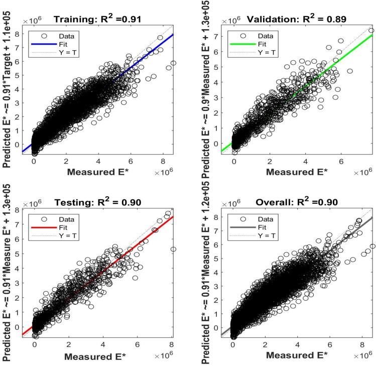
1

                                                                                      Session XXXX

   Development of Dynamic Modulus Predictive Model Using Artificial Neural
                             Network (ANN)
                         Prashanta Kumar Acharjee, Mena I. Souliman
                        Department of Civil and Environmental Engineering
                                The University of Texas at Tyler.

                                              Abstract
In Mechanistic-empirical Pavement Design Guide (MEPDG), dynamic modulus |E*| is identified as
a key property for Hot Mix Asphalt (HMA). Determining |E*| in the laboratory requires several days
of sophisticated testing procedures and expensive instruments. To bypass the long testing time,
sophisticated testing procedure, and expense, several multivariate regression analysis-based models
have been developed to predict the dynamic modulus from simpler materials properties and
volumetrics. Witczak 1999 and Modified Witczak 2006 are the two most widely used dynamic
modulus predictive models in the asphalt community. Several other regression-based models have
been developed earlier such as the Hirsch Model, the Law of Mixtures Parallel Model, and the
Resilient Modulus-based Model. The highest R2 value among all regression-based models is 0.87.
Using Artificial Neural Network (ANN) a |E*| prediction model is developed in this study. To train
the ANN model a dataset with 7400 data points is used, which is the same dataset used in the
Modified Witczak 2006 model development. The overall R2-value for the ANN model is 0.9 and is
better than other regression-based models. The weights and biases’ matrixes are reported to
reproduce the model for future use. This model can replace the existing regression-based model for
quick prediction of |E*| without performing any sophisticated test.

                                           Introduction
Dynamic modulus is defined as the relation between the maximum stress and maximum strain of a
viscoelastic material under continuous sinusoidal load. It is one of the most important properties to
design, analyze and evaluate the performance of Hot Mix Asphalt (HMA). Several predictive
models have been developed to predict the dynamic modulus from simple material properties and
volumetric. The previous generation regression-based model performs well enough to be
incorporated in the design manual. The equations developed through the regression-based model
are easy to use. But they are underperforming in extreme temperature and extreme dynamic
modulus values. The temperature also gets more importance in those multivariate regression-based
models. The new generation machine learning-based models are showing promise and performing
better in extreme. But they are not generating any equations to predict. To bridge the gap between
these two methods, in this study an Artificial Neural Network (ANN) model has been developed to
predict the dynamic modulus. Unlike the other ANN model, the wights and bias matrixes of the
model are reported. Therefore, the model is reproducible and can be used for different data set.

                      Proceedings of the 2022 ASEE Gulf-Southwest Annual Conference
                              Prairie View A&M University, Prairie View, TX
                       Copyright © 2022, American Society for Engineering Education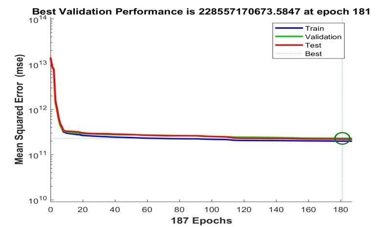
2

                                        Literature Review
The total length of roads in the United States of America is 2.3 million miles. Approximately 96% of
those roads have Hot Mix Asphalt (HMA) Surface1. Dynamic Modulus is an important property to
design, analyze and evaluate the performance of HMA surface. Vander Poel of the Shell Oil
Company introduced the term “stiffness” in the early 1950s2. As materials used in HMA are not
purely elastic, the stiffness of HMA depends on loading time and the temperature of the mix. To
represent the stiffness of HMA various parameters have been used, such as flexural stiffness, creep
compliance, relaxation modulus, resilient modulus, dynamic modulus, etc.3. The universally used
stiffness parameter is dynamic (complex) modulus (E*). One of the conclusions from the NCHRP 9-
19 project is that Dynamic Modulus (|E*|) is a good performance indicator for HMA design and was
recommended for Simple Performance Test (SPT)4. It is also recommended as quality control and
quality assurance parameter5. It is the key property for HMA in Mechanistic-empirical Pavement
Design Guide (MEPDG).

Dynamic Modulus |E*| is defined as the ratio between the amplitude of sinusoidal stress and
amplitude of sinusoidal strain at the same time and frequency. HMA is a visco-elastic material. It’s a
stress-strain relationship under continuous sinusoidal loading is defined by the dynamic modulus.
Determining Dynamic Modulus (|E*|) in the laboratory requires time, sophisticated procedures, and
an expensive testing machine. Therefore, various predictive model has been developed to predict
dynamic modulus from simple material properties and volumetric. Witczak 1999 and Modified
Witczak 2006 are the two most widely used dynamic modulus predictive models in the asphalt
community. Modified Witczak model was incorporated in MEPDG software along with the original
1999 Witczak equation6. Several other regression-based models have been developed earlier such as
the Hirsch Model, the Law of Mixtures Parallel Model, and the Resilient Modulus-based Model.
Several studies have concluded that regression-based multivariate models show significant scatter at
low or high dynamic modulus |E*| values and the accuracy falls flat in low and high-temperature
extremes7,8,9,10,11. Those models also tend to be dominated by the temperature as an input than the
other input parameters12. Table 1 shows the R2 values for all the regression models.
Table 1. Performance of Regression Bases Model for Predicting Dynamic Modulus13
                        Regression Model                       R2
          Hirch (arithmetic scale)                             0.871
          Revised Hirsch (arithmetic scale)                    0.874
          Revised Bari-Witczak (arithmetic scale)              0.875
          Al-Khateeb 1 (arithmetic scale)                      0.817
          Al-khateeb 2 (arithmetic scale)                      0.869
          NCHRP 1-40D (on logarithmic scale)                   0.332
          Simplified global (on logarithmic scale)             0.226
          Bari-Witczak (on logarithmic scale)                  0.584
          Revised Bari-Witczak (on logarithmic scale)          0.856

                      Proceedings of the 2022 ASEE Gulf-Southwest Annual Conference
                              Prairie View A&M University, Prairie View, TX
                       Copyright © 2022, American Society for Engineering Education
3
To overcome the shortcomings of the regression-based multivariate predictive model, Artificial
Neural Network (ANN) based model is also developed14,15. Using the same input variables as used
in the modified Witczak equation, the ANN models performed better in prediction. ANN models
showed better prediction accuracy at extreme lows and highs than the regression-based models.
They tend to have a better balance in giving priority to the temperature as an input than other input
parameters. Various other approaches have been developed like using machine learning and
computational micromechanics16,17,18. But all the models developed with machine learning worked
as a black box. Sometimes their weights and biases’ matrixes are not reported. Those models are not
reproducible. In this study, an ANN-based model is developed, and the weights and biases of the
model are reported. The main goal is to develop an ANN-based model which performs better than
the regression-based models. Therefore, the minimum number of hidden layers and neurons are
employed to build the model. The weights and biases are also reported. Therefore, the model can be
used on other datasets to predict dynamic modulus.
Developing Model with Artificial Neural Network
The dataset used in developing the Witczak-Bari model is also used in this study in the training,
validation, and testing process of the model. 7400 input data is used to predict the output data. The
7400-input data was collected from 346 mixes. The input variables were chosen as the same
variables used in the Modified Witczak equation. The number of Input variables was eight and
dynamic modulus was the target output in the training process. 7400 unique E* with eight input
variables were fed into the network. Table 2 is showing all the variables in the training process.
Table 2. Variables Used in the Model
Variable Name Notation Unit
Percentage of aggregates (by weight) retained on ¾ inch sieve %
Percentage of aggregates (by weight) retained on 3/8 inch sieve 38 %
Percentage of aggregates (by weight) retained on #4 sieve 4 %
Percentage of aggregates (by weight) passing through #200-inch sieve 200 %
sieve
Percentage of air voids (by volume) Va %
Percentage of effective asphalt content (by volume) Vbeff %
Dynamic shear modulus of binder |Gb*| psi
Phase Angle of binder associated with |Gb| (b). degree
Dynamic modulus E* psi
Different interconnected neurons work together to solve complex problems in Artificial Neural
networks. The greater number of neurons and hidden layers give better results. But an increased
number of neurons and hidden layers produce an overfitted model which does not perform well
outside the training database. Therefore, one hidden layer is typically sufficient to solve most non-
linear problems19. At first, the model was trained with one neuron in one hidden layer. The R2 value
was not sufficient for the model with a single neuron. Then the number of neurons was increased. If
the R2 value was not sufficient, then the number of neurons was increased again. After repeating this
process for few times, the desired R2 was achieved with 20 neurons in one hidden layer.
Out of the 7400 data points, 70% of the data was randomly selected and used as a training data set.
The model was trained with the 5180 data points. The R2 is 0.91 for the training dataset. The R2 for
Proceedings of the 2022 ASEE Gulf-Southwest Annual Conference
Prairie View A&M University, Prairie View, TX
Copyright © 2022, American Society for Engineering Education4
the validation dataset was 0.89. 15% of the data points, which is 1110 points were used in the model
validation process. For model validation, the main target was to optimize the Mean Squared Error
(MSE). When the MSE value reached the minimum value, the training was stopped. Figure 1 shows
that the least MSE value was reached after 187 iterations. The least MSE value was 2.2x 10¹¹.
Figure 1. Validation of the ANN model in 187 epochs.
After completing the training and validation process, the model was tested on the remaining 15%
data points. These 1110 data points were unknown to the model. The testing data was kept away
from the model before testing. This testing process made the model robust against unknown data.
The R2 for testing was 0.90. Testing the model against unknown data protects the model from
overfitting the model with the training dataset. Figure 2 shows that all three R2 values in the training,
validation and testing process are fairly close. The overall R2 for the model is 0.9. This is better than
any regression-based prediction model mentioned in Table1.
Figure 2. R2 values in Training, Validation, Testing and Overall
Proceedings of the 2022 ASEE Gulf-Southwest Annual Conference
Prairie View A&M University, Prairie View, TX
Copyright © 2022, American Society for Engineering Education5
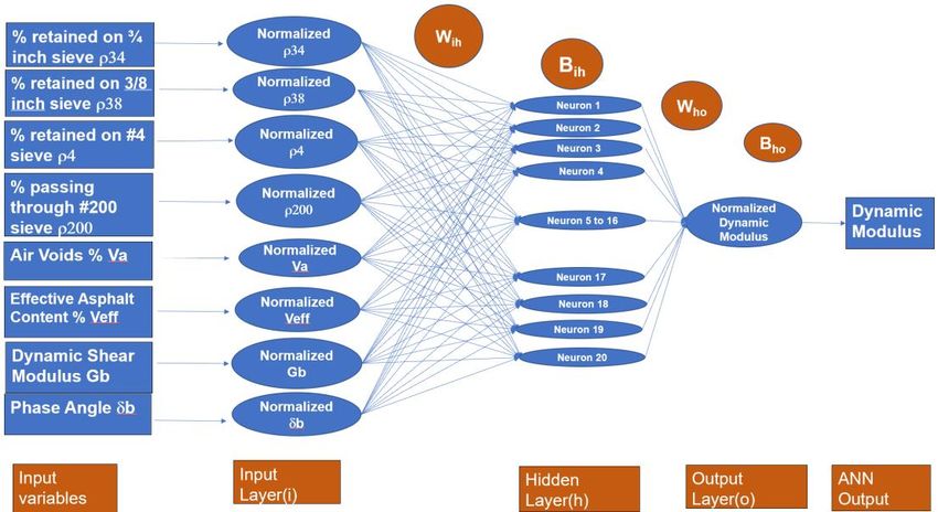
The ANN-based model is run by matrixes of weights and biases. The normalized input variables are
multiplied by the weight matrix Wih and the bias matrix bih is added with the product. After that, the
product from the hidden layer is multiplied by the weight matrix Who, and bias bho is added with the
product. In this step, a normalized out is gained from the model. After denormalizing the output, the
model provides the target output. Figure 3 shows the architecture of the ANN model developed in
this study. All the matrixes for weights and biases are also reported below.
Figure 3. Architecture of the ANN-based Dynamic Modulus Prediction Model
0.29215 2.85901 -0.07638 -1.24597 0.93330 3.33122 -0.08884 -0.26267
0.88552 3.74619 -6.54191 -2.04369 -1.19882 -7.72302 1.91874 -1.23025
-0.13862 0.78280 0.58535 -0.56057 2.39711 0.00381 0.44160 0.70837
Weights -0.87278 0.75418 1.05796 -1.54662 -0.50222 -1.58830 -0.62947 -0.37123
for -6.59999 -6.11600 -16.45912 -12.85108 3.35584 5.13716 0.31735 -0.98884
Input to -3.68108 0.32216 4.89963 -4.27105 -0.91915 -0.26141 0.58768 0.09217
Hidden -0.19185 -3.52012 0.11113 1.07106 -0.90254 -3.64307 -0.00770 0.22774
Layer -1.31807 -9.47328 -3.66345 0.50221 0.22424 -6.62614 -0.55127 0.97766
Wih = -2.17382 1.19072 7.19416 2.66379 4.36667 -1.84596 1.35009 -0.73111
-1.26529 -4.39237 7.08120 -5.04528 4.82078 -4.69730 -0.06433 -0.19913
-1.46441 -9.74722 9.28093 -6.63405 -0.73764 -4.63959 0.20348 0.38662
0.08794 -0.06233 -0.06126 -0.11862 0.10494 0.24015 0.71473 -1.33418
-1.92693 2.43979 -8.60489 -8.26152 -0.63829 0.43640 0.28198 0.01332
6.30896 6.44113 16.17857 13.19441 -3.35549 -4.95544 -0.30429 0.97204
16.55955 0.14000 -4.35588 2.37729 -2.96943 -4.73150 -11.73132 -0.21176
0.16664 -0.45681 5.49950 6.69828 2.22188 0.10980 -0.40303 0.13905
-19.41615 18.64156 -14.05268 2.14252 3.79068 1.08215 -0.55314 1.29301
-1.63538 14.18238 -2.40314 -0.77948 2.40239 -4.10070 0.79061 -2.16614
0.09570 -0.05574 -0.06413 -0.12570 0.11467 0.28183 1.04686 -1.43687
-0.09871 0.07992 0.06293 0.13594 -0.10934 -0.27419 -0.29971 1.62902
Proceedings of the 2022 ASEE Gulf-Southwest Annual Conference
Prairie View A&M University, Prairie View, TX
Copyright © 2022, American Society for Engineering Education6
-0.50427 3.624678
-4.94848 -0.16163
3.62468 0.918998 -0.27898
-0.2268 Weights 0.42097 Biases for
-2.15554 for Hidden 4.846017 Hidden
-4.94848
Biases for Input Layer to Layer to
3.749635 -0.62366
Output Output
to Hidden Layer 0.321625 3.58437
Layer
-0.16163 0.079402 -0.17146 Layer
bih = -0.80196 Who = 0.114938 bho= -1.28448
B1 = -2.96723 0.124402
0.91900 -5.81389 -0.18644
1.847841 23.7495
-0.27898 -0.0355 -0.22211
2.273769 4.895425
1.500197 -0.04863
-0.22680 0.303827 -0.27493
-0.90465 0.156574
0.42097 -9.22379 0.213876
1.883526 -8.96053
-1.85333 13.29923
-2.15554
The number of rows and columns in the first weight matrix Wih represents the size of the network.
4.84602
The number of columns represents the number of input variables used. Here it is 8. The number of
rows represents the neurons, used in the network. Here, the number of neurons used is 20. The input
variables3.74964
are put into the network after normalizing every input between the [-1,1] range.
Normalizing the input protects the training process from overweighing the variable with a large
value. After normalization, all variables are in the range of [-1,1]. The input variables are multiplied
-0.62366
by the first weight matrix Wih and the bias matrix bih is also added. The output from this process
enters into the hidden layer and every value in the hidden layer is activated with the hyperbolic Tan
function.0.32162
From the hidden layer, the inputs are multiplied by the second weight matrix Who, and bias
bho is also added. After that the value is denormalized and the model gives the outcome. All the
wights and the model in this study can be reproduced.
3.58437
Summary and Conclusion
0.07940
The ANN model in this study performed better than the existing regression-based models. The
weights and biases’ matrixes can be used to reproduce the model for further use. Even an equation
-0.17146 Tangent function can be produced from the matrixes. But it will be a lengthy
with hyperbolic
equation as the number of equations will represent the number of lines in the equation. Future
studies will tackle this issue with less number of neurons. One of the limitations of ANN based-
model is-0.80196
that ANN can not extrapolate data. Therefore, it does not perform outside the range of the
training dataset. Therefore, before applying this model on to any data, the range of the values of the
variables0.11494
should be checked first. But 7400 points cover a wide range. With R2 = 0.9, this model can
be used to predict dynamic modulus without going through laboratory procedures.
-1.28448
-2.96723
Proceedings of the 2022 ASEE Gulf-Southwest Annual Conference
0.12440 Prairie View A&M University, Prairie View, TX
Copyright © 2022, American Society for Engineering Education
-5.81389
-0.186447
References
1. Roberts, F. L., Kandhal, P. S., Brown, E. R., Lee, D. Y., & Kennedy, T. W. (1991). Hot mix asphalt materials,
mixture design and construction.
2. Van Poel, C. D. (1954). A general system describing the visco‐elastic properties of bitumens and its relation to
routine test data. Journal of applied chemistry, 4(5), 221-236.
3. Bari, J. (2005). Development of a new revised version of the Witczak E* predictive models for hot mix asphalt
mixtures. Arizona State University.
4. Witczak, M. W., Quintas, H. V., Kaloush, K., Pellinen, T., & Elbasyouny, M. (2000). Simple performance test:
Test results and recommendations. Interim Report. Arizona: Arizona State University.
5. Bonaquist, R. F., Christensen, D. W., & Stump, W. (2003). Simple performance tester for Superpave mix
design: First-article development and evaluation (Vol. 513). Transportation Research Board.
6. Brown, S. F., Darter, M., Larson, G., Witczak, M., & El-Basyouny, M. M. (2006). Independent review of the"
mechanistic-empirical pavement design guide" and software. NCHRP research results digest, (307).
7. Pellinen, T. K. (2001). Investigation of the use of dynamic modulus as an indicator of hot-mix asphalt
peformance. Arizona State University.
8. Schwartz, C. W. (2005, January). Evaluation of the Witczak dynamic modulus prediction model. In
Proceedings of the 84th Annual Meeting of the Transportation Research Board, Washington, DC (No. 05-
2112).
9. Dongre, R., Myers, L., D'Angelo, J., Paugh, C., & Gudimettla, J. (2005). Field evaluation of Witczak and
Hirsch models for predicting dynamic modulus of hot-mix asphalt (with discussion). Journal of the Association
of Asphalt Paving Technologists, 74.
10. Al-Khateeb, G., Shenoy, A., Gibson, N., & Harman, T. (2006). A new simplistic model for dynamic modulus
predictions of asphalt paving mixtures. Journal of the Association of Asphalt Paving Technologists, 75.
11. Azari, H., Al-Khateeb, G., Shenoy, A., & Gibson, N. (2007). Comparison of Simple Performance Test| E*| of
Accelerated Loading Facility Mixtures and Prediction| E*| Use of NCHRP 1-37A and Witczak's New
Equations. Transportation Research Record, 1998(1), 1-9.
12. Schwartz, C. W. (2005). “Evaluation of the Witczak dynamic modulus prediction model.” Proc., 84th Annual
Meeting of the Transportation Research Board (CD-ROM), Transportation Research Board, Washington, D.C.
13. Barugahare, J., Amirkhanian, A. N., Xiao, F., & Amirkhanian, S. N. (2020). ANN-based dynamic modulus
models of asphalt mixtures with similar input variables as Hirsch and Witczak models. International Journal of
Pavement Engineering, 1-11.
14. Ceylan, H., Kim, S., & Gopalakrishnan, K. (2007). Hot mix asphalt dynamic modulus prediction models using
neural networks approach.
15. Ceylan, H., Gopalakrishnan, K., & Kim, S. (2008). Advanced approaches to hot-mix asphalt dynamic modulus
prediction. Canadian Journal of Civil Engineering, 35(7), 699-707.
16. Behnood, A., & Daneshvar, D. (2020). A machine learning study of the dynamic modulus of asphalt concretes:
An application of M5P model tree algorithm. Construction and Building Materials, 262, 120544.
17. Behnood, A., & Golafshani, E. M. (2021). Predicting the dynamic modulus of asphalt mixture using machine
learning techniques: An application of multi biogeography-based programming. Construction and Building
Materials, 266, 120983.
18. Karki, P., Kim, Y. R., & Little, D. N. (2015). Dynamic modulus prediction of asphalt concrete mixtures through
computational micromechanics. Transportation Research Record, 2507(1), 1-9.
19. Chan, V. and C.W. Chan. Development and application of an algorithm for extracting multiple linear regression
equations from artificial neural networks for non-linear regression problems. In Cognitive Informatics &
Cognitive Computing (ICCI CC), 2016 IEEE 15th International Conference (pp. 479-488).
Prashanta Kumar Acharjee
Prashanta Kumar Acharjee is currently working as a graduate research assistant at the University of Texas at Tyler. After
graduating from Bangladesh University of Engineering and Technology he is perusing his Masters at UT Tyler. His
research interest is broadly in transportation engineering.
Proceedings of the 2022 ASEE Gulf-Southwest Annual Conference
Prairie View A&M University, Prairie View, TX
Copyright © 2022, American Society for Engineering Education8
Mena I. Souliman
Dr. Souliman currently serves as an Associate Professor of the Civil and Environmental Engineering Department in the
University of Texas at Tyler. His experience is concentrated on pavement materials design, Fatigue Endurance Limit of
Asphalt Mixtures, Reclaimed Asphalt Pavement (RAP) mixtures, aggregate quality, field performance evaluation,
maintenance and rehabilitation techniques, pavement management systems, cement-treated bases, statistical analyses,
modeling, and computer applications in civil engineering. Dr. Souliman is a registered engineer in the state of Texas. He
has more than 100 technical publications, conference papers, and reports in the field of pavement and aggregate testing,
characterization, and field monitoring. He is the recipient of the lifetime International Road Federation Fellowship in
2009.
Proceedings of the 2022 ASEE Gulf-Southwest Annual Conference
Prairie View A&M University, Prairie View, TX
Copyright © 2022, American Society for Engineering EducationYou can also read