Development of Natural Gas Supply Curves for EPA Platform v6 - US EPA
←
→
Page content transcription
If your browser does not render page correctly, please read the page content below
8.      Development of Natural Gas Supply Curves for EPA Platform v6
8.1   Introduction

Natural gas supply curves and regional basis are key inputs to IPM and are developed using ICF’s Gas
Market Model (GMM). ICF develops and maintains the GMM for use by both private and public sector
clients. The model has been used to examine strategic issues relating to natural gas supply, pipeline
infrastructure, pricing, and demand characteristics.

Like IPM, GMM is a large-scale linear programming model that incorporates a detailed representation of
gas supply characteristics, demand characteristics, and an integrating pipeline transportation model to
develop forecasts of gas supply, demand, prices, and flows. GMM is a full supply/demand equilibrium
model of the North American gas market. The model solves for monthly natural gas prices throughout
North America, given different supply/demand conditions, the assumptions for which are specified by
each scenario. Overall, the model solves for monthly market clearing prices by considering the
interaction between supply and demand at each node in the model.

On the supply side, prices are determined by production and storage price curves that reflect prices as a
function of production and storage utilization. Prices are also influenced by “pipeline discount” curves,
which reflect the change in basis or the marginal value of gas transmission as a function of load factor.
On the demand side, prices are represented by a curve that captures the fuel-switching behavior of end-
users at different price levels. The model balances supply and demand at all nodes in the model at the
market clearing prices. ICF updates GMM model inputs and performs calibration of the model on a
monthly basis to ensure the model reliably reflects historical gas market behavior. Figure 8-1 shows the
supply side of the calculation in GMM, and Figure 8-2 shows the interaction of IPM and GMM.

                          Figure 8-1 GMM Gas Quantity and Price Response

                                                   8-1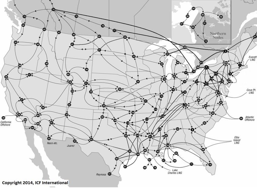
Figure 8-2 IPM/GMM Interaction
Natural Gas Modeling Power Sector Modeling
Natural Gas Supply Curves
Integrated
Integrated
Gas Market Planning
Model (GMM) Planning
Model (IPM)
Model
Power Sector Gas Demand
Activities Activities
Activities
Assumption
Assumption Updates
Updates Assumption Updates
Assumption Updates
Scenario Analysis Peer Review
Scenario Analysis
Scenario Analysis Scenario Analysis
Products Products
Natural Gas Projections Environmental Policy Assessments
Natural Gas Supply Curves Inputs for Air Quality Modeling
To establish gas supply curves in EPA’s Platform v6, both GMM and IPM are operated in tandem and are
iterated to develop a consistent Henry Hub gas price and total gas demand forecast that informs the
derivation of those supply curves. In subsequent analyses using IPM, EPA’s Platform v6 will continue to
use these originally derived gas supply curves (without necessitating re-modeling in GMM), unless
otherwise documented with a given scenario analysis. EPA’s Platform v6 uses natural gas market
assumptions in power market modeling as follows:
IPM takes the natural gas supply curves, which are developed based on GMM outputs and
specified as a function of Henry Hub prices.
For each year, three sets of seasonal natural gas transportation differentials (summer, winter, and
winter shoulder) are added to the supply curves to generate the final delivered curves by IPM
region.
IPM projects the power sector’s demand for natural gas. The natural gas demand is compared to
the supply curve to find the market-clearing price for natural gas.
IPM’s linear programming formulation takes into consideration the gas supply curves as well as
coal supply curves and detailed power plant modeling in determining electric market equilibrium
conditions. Oil usage is modeled as a function of price, which is exogenously supplied to IPM.
This chapter is divided in the following sections. The chapter starts with a brief synopsis of GMM, the
primary tool used for generating the natural gas supply curves. This is followed by detailed discussions of
modeling methodologies and data used in GMM. The methodologies and data description are grouped in
the following five sections:
i) Resources data and reservoir description
ii) Treatment of frontier resources and exports
iii) Exploration and production technology characterization
iv) Oil prices
v) Demand assumptions
This is followed by discussion of natural gas assumptions and supply curves used for EPA Platform v6.
8-2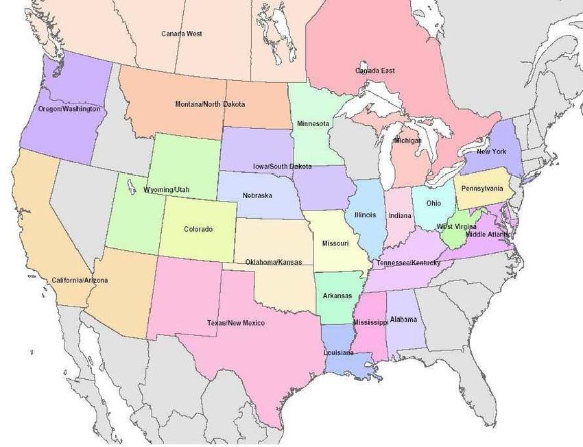
8.2   Brief Synopsis of GMM

ICF’s integrated natural gas model, GMM, is designed to perform comprehensive assessments of the
entire North American gas flow pattern. It is a large-scale, dynamic linear program that models economic
decision-making to minimize the overall cost of meeting natural gas demand. GMM is reliable and
efficient in analyzing the broad range of natural gas market issues.

                               Figure 8-3 Geographic Coverage of GMM

Important features of GMM are described below.

Natural Gas Market Prices in GMM are determined by the marginal (or incremental) value of natural gas
at 121 regional market centers. Prices are “at the margin”, not “average”. Marginal prices do not
translate directly into pipeline or utility revenues. Prices represent “market center” prices as opposed to
delivered prices. Gas prices are determined by the balance of supply and demand in a regional
marketplace. Supply is determined considering both availability of natural gas deliverability at the
wellhead, the transportation capacity and cost to deliver gas to market centers.

Natural gas production prices are determined from spot gas price curves that yield price as a function of
deliverability utilization: Curves reflect price for gas delivered into the transmission system (including
gathering cost). Gas storage withdrawal price curves are added to the production price curves during the
withdrawal season. Pipeline value curves are then added to yield a total supply curve for a node. The
intersection of the supply curve and the demand curve (including net storage injections) yields the
marginal price at a node. Price is set by the demand curve when all available supply is utilized.

Demand is modeled for residential, commercial, industrial, and power sectors for each of the 121 nodes.
GMM solves for gas demand across different sectors, given economic growth, weather, and the level of
price competition between gas and oil. Econometric equations define demand by sector. The industrial

                                                    8-3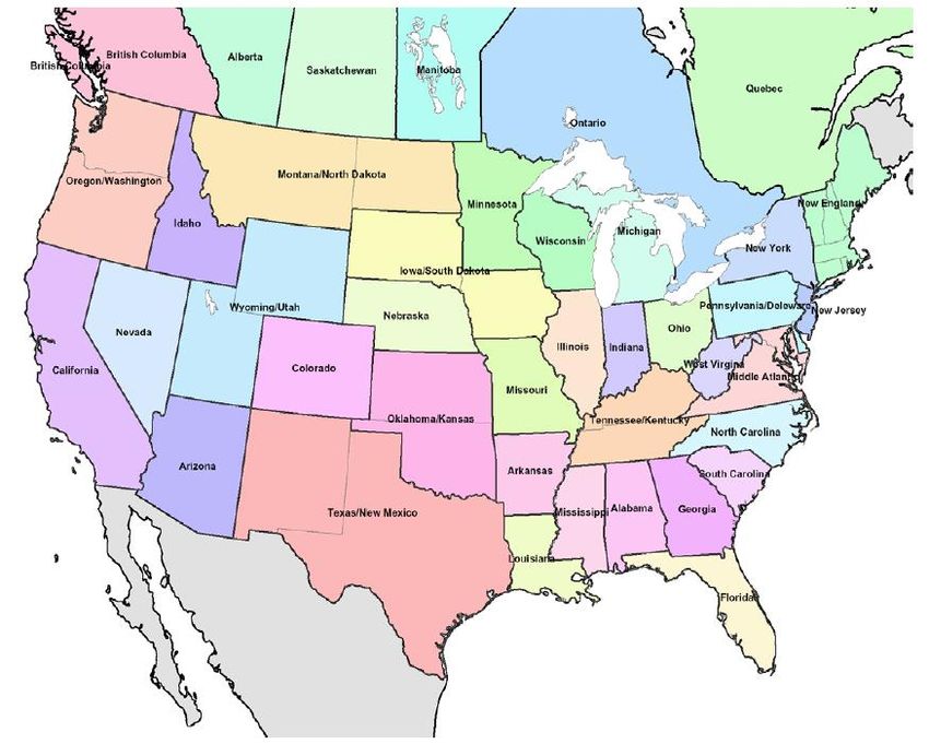
and power sectors incorporate fuel competition, dispatch decisions, new power plant builds, economic
growth, and weather. GMM solves the power generation dispatch on a regional basis to determine the
amount of gas used in power generation, which is allocated along with end-use gas demand to model
nodes. GMM iterates with IPM to better capture electric sector demand for natural gas.
Electric generation is modeled regionally with plant dispatch based upon operating cost. Competing
power generation technologies are evaluated on a full-cost basis to determine lowest cost capacity
additions.
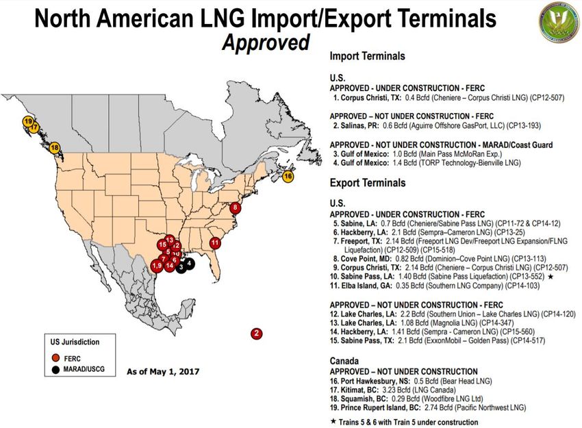
Transportation is modeled by over 423 transportation links between the nodes, balancing seasonal,
sectoral, and regional demand and prices, including pipeline tariffs and capacity allocation. Node
structure developed to reflect points of change or influence on the pipeline system. These points include:
major demand and supply centers, pipeline hubs and market centers, and points of divergence in pipeline
corridors. The pipeline network is largely represented as bundles of pipes, though in some regions
individual pipes are represented. Gas moves over the network at variable cost. The variable cost as a
function of pipeline throughput (i.e., pipeline discount curve) is used to determine the market value of
capacity (i.e., the transportation basis) for each period in the forecast for each pipeline link.
Figure 8-4 Example Pipeline Discount Curve
The upper end of discount curve may be shifted by additions of new pipeline capacity. The shift depends
on expansion tariff relative to pre-expansion tariff and pricing of expansion (incremental or rolled-in).
Curves have been fit to basis observed from actual gas prices and to annual load factors. Pipeline
discount curve parameters can also be changed over time to reflect regulatory changes that affect
pipeline values.
Pipeline capacity expansions address the physical constraints of transporting gas from supply regions to
demand regions. They therefore contribute to determining the supply curves and seasonal basis. For the
near–term, pipeline capacity expansions are input to GMM based on identifiable, near-term development
plans and ICF’s market assessment. For the longer term, new “generic” pipeline capacity is added in
GMM when the market value of the added capacity exceeds its cost. Generic pipeline capacity in the
model is added starting 2023 and it increases in 2025 and beyond as the natural gas markets grow.
ICF includes projects that satisfy certain criteria in its analysis. The criteria are listed below.
• First Criteria: The project is already under construction;
8-4
OR
•       Second Criteria: The project has the necessary approvals to proceed from FERC and other
relevant regulatory proceedings;
                          OR
•       Third Criteria: The project has been filed with FERC and has the necessary firm shipper
commitments;
                          OR
•       Fourth Criteria: The project has been filed with FERC and does not have the necessary shipper
commitments, but does appear to have sufficient market support;
                          OR
•       Fifth Criteria: The project has NOT yet been filed with FERC, but appears to have sufficient
market support.

For the fourth and fifth criteria, ICF typically considers supply growth directly upstream of the project,
market growth for markets that are relevant to the project’s delivery point/s, and basis differentials that
exceed the per unit cost of pipeline expansion as indicators of market support. If the indicators are all
positive, ICF will add the project as a “generic” project and size it based on the level of market support. In
the case in which there are multiple generic projects for a single GMM link, the generic projects will be
sized in aggregate based on the total level of market support for expansion of the link. Generic projects
are classified as such until one of the first three criteria are satisfied.

For certain markets like New York, New Jersey and New England, ICF looks closely at regulatory support
for the project which could override the criteria above in determining the pipeline additions in GMM. For
example, if a project like Constitution pipeline has been denied water permits even though it has broad
market support, ICF does not include it in its base case.

Pipeline cost assumptions used in GMM have been derived by considering data from Oil and Gas Journal
(OGJ) surveys of pipeline projects. Using regression analysis of the OGJ data across years, we
determined an average U.S. pipeline cost of $183,000 per inch-mile for 2017 (in 2016 dollars) for large
gas transmission pipelines. The pipeline cost for future years is kept flat in real terms post 2017.
Regional cost multipliers have also been derived from OGJ data as the pipeline costs vary by region.
Cost multipliers can be different across regions; for example, costs are relatively high in the Northeast
where projects have been very difficult and time consuming to construct.

Supply is modeled by using node-level natural gas deliverability or supply capability, including import and
export levels while accounting for gas storage injections and withdrawals at different gas prices. Total
supply in the United States comes from three sources: production from natural gas fields located in the
lower 48 states, Canadian imports, Alaska, and LNG imports. Natural gas production activity is
represented in 82 of the 121 Model nodes where historical production has occurred, or where future
production appears likely. The “base trend” for deliverability and gas price are developed from ICF’s
resource assessment using the Hydrocarbon Supply Model and a long-term “marker price”. If the monthly
solution price deviates from the “marker price”, future exploration and production (E&P) activity is
adjusted. Deliverability responds to prices, with a lag of 2 to 18 months.

The components of supply (i.e., gas deliverability, storage withdrawals, supplemental gas, LNG imports,
and Mexican imports) are balanced against demand (i.e., end-use demand, power generation gas
demand, LNG exports, and Mexican exports) at each of the nodes and gas prices are solved for in the
market simulation module.

Natural Gas Storage activity is represented for 24 U.S. and two Canadian storage regions, with activity
allocated to individual nodes based on historical field level storage capacity. Regional differences in the
physical and market characteristics of storage are captured in the storage injection and withdrawal
relationships separately estimated for each region:

    -   Differences between market area storage and supply area storage.

                                                     8-5
- Differences between regions with primarily depleted field storage and regions with primarily
aquifer storage.
Net monthly withdrawals are calculated from a “storage supply curve” that reflects the level of withdrawals
relative to gas prices. The curve has been fit to actual historical data. Net monthly injections are
calculated from econometrically fit relationships that consider working gas levels, gas prices, and weather
(i.e., cooling degree days). The level of gas storage withdrawals and injections are calculated within the
supply and demand balance algorithm based on working gas levels, gas prices, and extraction/injection
rates and costs.
Figure 8-5 GMM Natural Gas Storage Regions
Storage levels have an impact on GMM’s seasonal basis differentials, which are an important component
in constructing the gas supply curves and/or basis differentials that are then input into IPM. The arbitrage
value of storage is driven by the seasonal difference in the supply-area gas prices plus the seasonal
difference in pipeline transportation value. Storage expansions (or increased utilization of existing
storage) decreases seasonal basis differentials in the region surrounding the storage facilities.
8.3 Resources Data and Reservoir Description
This section describes the approach used in GMM and documents the changes to the resource data and
reservoir characterization work conducted for EPA Platform v6.
8.3.1 U.S. Resources and Reserves
This section describes the U.S. resource data sources and methodology used in GMM for EPA Platform
v6.
Current U.S. and Canada gas production is from over 400 trillion cubic feet (Tcf) of proven gas reserves.
ICF assumes that the U.S. and Canada natural gas resource base totals roughly 3,500 Tcf of unproved
8-6plus discovered but undeveloped gas resource. This can supply the U.S. and Canada gas markets for
over 100 years (at current consumption levels). Shale gas accounts for over 50 percent of remaining
recoverable gas resources. No significant restrictions on well permitting and fracturing are assumed
beyond restrictions that are currently in place.
Data sources: Conventional resource base assessment is based on data from the U.S. Geological Survey
(USGS), Minerals Management Service (MMS), and Canadian Gas Potential Committee (CGPC) using
ICF’s Hydrocarbon Supply Model (HSM).
In the area of unconventional gas, ICF has worked for many years with the Gas Research Institute
(GRI)/Gas Technology Institute (GTI) to develop a database of tight gas, coalbed methane, and Devonian
Shale reservoirs in the U.S. and Canada. Along with USGS assessments of continuous plays, the
database was used to help develop the HSM’s “cells”, which represent resources in a specific geographic
area, characterizing the unconventional resource in each basin, historical unconventional reserves
estimates and typical decline curves. ICF has recently revised the unconventional gas resource
assessments based on new gas industry information on the geology, well production characteristics, and
costs. The new assessments include major shale units such as the Fort Worth Barnett Shale, the
Marcellus Shale, the Haynesville Shale, and Western Canada shale plays. ICF has built up a database
on gas compositions in the United States and has merged that data with production data to allow the
analysis of net versus raw gas production.
Resources are divided into three general categories: new fields/new pools, field appreciation, and
unconventional gas. The methodology for resource characterization and economic evaluation differs for
each.
New Fields
Conventional new discoveries are characterized by size class. For the United States, the number of
fields within a size class is broken down into oil fields, high permeability gas fields, and low permeability
gas fields based on the expected occurrence of each type of field within the region and interval being
modeled. The fields are characterized further as having a hydrocarbon make-up containing a certain
percent each of crude oil, dry natural gas, and natural gas liquids. In Canada, fields are oil, sweet
nonassociated gas, or sour nonassociated gas.
The methodology uses a modified “Arps-Roberts” equation to estimate the rate at which new fields are
discovered. The fundamental theory behind the find-rate methodology is that the probability of finding a
field is proportional to the field's size as measured by its areal extent, which is highly correlated to the
field's level of reserves. For this reason, larger fields tend to be found earlier in the discovery process
than smaller fields. The new equation developed by ICF accurately tracks discovery rates for mid- to
small-size fields. Since these are the only fields left to be discovered in many mature areas, the more
accurate find-rate representation is an important component in analyzing the economics of exploration
activity in these areas.
An economic evaluation is made in the model each year for potential new field exploration programs
using a standard discounted after-tax discounted cash flow (DCF) analysis. This DCF analysis takes into
account how many fields of each type are expected to be found and economics of developing each. The
economic decision to develop a field is made using “sunk cost” economics where the discovery cost is
ignored and only time-forward development costs and production revenues are considered. However, the
model’s decision to begin an exploration program includes all exploration and development costs.
Field Appreciation
Field appreciation refers to potential resources that can be proved from already discovered fields. These
inventories are referred to as appreciation, growth-to-known or “probables.” The inventories of probables
are increased due to expected future appreciation due to many factors that include higher recovery
percentages of the gas in-place resulting from infill drilling and application of improved technology and
experience gained in the course of developing and operating the field.
8-7Unconventional Gas
The ICF assessment method for shale gas is a “bottom-up” approach that first generates estimates of
unrisked and risked gas-in-place (GIP) from maps of depth, thickness, organic content, and thermal
maturity. Then, ICF uses a different model to estimate well recoveries and production profiles. Unrisked
GIP is the amount of original gas-in-place determined to be present based upon geological factors—
without risk reductions. “Risked GIP” includes a factor to reduce the total gas volume based on proximity
to existing production and geologic factors such as net thickness (e.g., remote areas, thinner areas, and
areas of high thermal maturity have higher risk). ICF calibrates expected well recoveries with specific
geological settings to actual well recoveries by using a rigorous method of analysis of historical well data.
To estimate the contributions of changing technologies ICF employs the “learning curve” concept used in
several industries. The “learning curve” describes the aggregate influence of learning and new
technologies as having a certain percent effect on a key productivity measure (for example cost per unit
of output or feet drilled per rig per day) for each doubling of cumulative output volume or other measure of
industry/technology maturity. The learning curve shows that advances are rapid (measured as percent
improvement per period of time) in the early stages when industries or technologies are immature and
that those advances decline through time as the industry or technology matures. Generally speaking, we
find the learning curve effect is roughly 20 percent per doubling of cumulative wells.
Major Unconventional Natural Gas Categories
Definition of Unconventional Gas: Quantities of natural gas that occur in continuous,
widespread accumulations in low quality reservoir rocks (including low permeability or tight
gas, coalbed methane, and shale gas), that are produced through wellbores but require
advanced technologies or procedures for economic production.
Tight Gas is defined as natural gas from gas-bearing sandstones or carbonates with an in situ
permeability (flow rate capability) to gas of less than 0.1 millidarcy. Many tight gas sands have
in situ permeability as low as 0.001 millidarcy. Wells are typically vertical or directional and
require artificial stimulation.
Coalbed Methane is defined as natural gas produced from coal seams. The coal acts as both
the source and reservoir for the methane. Wells are typically vertical but can be horizontal.
Some coals are wet and require water removal to produce the gas, while others are dry.
Shale Gas is defined as natural gas from shale formations. The shale acts as both the source
and reservoir for the methane. Older shale gas wells were vertical while more recent wells are
primarily horizontal with artificial stimulation. Only shale formations with certain characteristics
will produce gas.
Shale Oil with Associated Gas is defined as associated gas from oil shale in horizontal
drilling plays such as the Bakken in the Williston Basin. The gas is produced through
boreholes along with the oil.
8.3.2 Upstream Cost and Technology Factors
In ICF’s methodology, supply technology advancements effects are represented in three categories:
Improved exploratory success rates
Cost reductions of platform, drilling, and other components
Improved recovery per well
8-8These factors are included in the model by region and type of gas and represent several dozen actual
model parameters. ICF’s database contains base year cost for wells, platforms, operations and
maintenance, and other relevant cost items.
Figure 8-6 GMM U.S. and Canada Projected Gas Production by Source
8.3.3 Historical Gas Production
ICF consistently updates the production and resource data that it used for EPA Platform v6. The
historical production data for the model comes from PointLogic. An example comparison of production
forecasts for the San Juan and Raton basins is shown in Figure 8-7.
8-9Figure 8-7 Production Comparison for San Juan and Raton Basins
8.3.4 Treatment of Frontier Resources and Exports
Arctic Projects
GMM does not have resources located in frontier regions. Arctic projects (specifically Alaska and
Mackenzie Valley gas pipelines) are not included in our projection.
Existing and Potential Liquefied Natural Gas (LNG) Terminals
LNG is natural gas that has been transformed to a liquid by super-cooling it to minus 260 degrees
Fahrenheit, reducing its volume by a factor of 600. LNG is then shipped on board special carriers, and
the process is reversed at a receiving facility with the re-gasified product delivered via pipeline. Based on
current global LNG market conditions, ICF assumes that the six U.S. LNG terminals currently under
construction are completed and expanded in future. Those terminals are Sabine Pass, Freeport, Cove
Point, Cameron, Corpus Christi, and Elba Island. By 2020, ICF projects U.S. LNG export capacity will be
10.3 billion cubic feet per day (Bcfd). Given the near-term low oil price expectations, we project that
North American export terminal capacity utilization will average about 63% through 2020. U.S. export
volumes are projected to approach six Bcfd by 2020. ICF projects that the capacity utilization will
increase to over 80% by 2024. In addition to the U.S. trains currently under construction, ICF assumes
an additional 5.8 Bcfd of export capacity will come online in North America between 2020 and 2035. ICF
assumes that only one export facility will be built in British Columbia: Woodfibre (0.3 Bcfd).
8-10Figure 8-8 Existing and Proposed Marine LNG Terminals as of May 2017
Figure 8-9 LNG Export Volumes versus Capacity
8-11Pipeline Exports to Mexico
Mexico’s demand for natural gas continues to rise, while its domestic production has been declining.
Since 2010, Mexico’s imports of U.S. gas have gone up over 300%, reaching 3.9 Bcfd in 2016. As
Mexico continues to add gas-fired generation and sponsor new pipelines from the U.S., exports will
continue to grow. ICF projects that exports will reach 8 Bcfd by 2035.
Figure 8-10 U.S. Pipeline Exports to Mexico
8.4 Oil Prices
Natural gas prices and LNG export levels are forecasted by taking into account oil prices. The following
section contains discussions about the crude oil price assumptions used for EPA Platform v6.
ICF uses the Refiner Acquisition Cost of Crude Oil (RACC) price as an oil price input to GMM. The
RACC price is a term commonly used in discussing crude oil. It is the cost of crude oil to the refiner,
including transportation and fees. For the long-term, ICF projects a slow recovery in oil prices to an
equilibrium marginal production cost of $75/bbl (in $2016). The residual oil price averages between 70
and 100 percent of the RACC price on a dollar per Btu basis. This is the price used to determine
switching in the industrial sector. Figure 8-11 shows the ICF RACC price projection.
8-12Figure 8-11 Refiners’ Acquisition Cost of Crude (RACC)
8.5 Demand Assumptions
Gas demand is calculated by sets of algorithms and equations for each sector and region. The model
calculates monthly “real-time consumption”, not “billed volumes.” Demand reported by DOE/EIA
represents billed volumes, which is time-lagged. Recent DOE/EIA and Statistics Canada data have been
considered in the calibration of the model. However, the historical data represents ICF’s backcast of the
market. ICF performs market reconnaissance and data analysis each month to support the GMM
calibration. GMM models natural gas demand in four end-use sectors: residential, commercial, industrial,
and power generation.
Residential/Commercial gas demand calculated from regional equations fit econometrically to weather,
economic growth, and price elasticity. The 41 regions for which residential/commercial demand are
calculated are shown in Figure 8-12. Regression analysis was separately completed for each sector for
34 Lower-48 and 7 Canadian regions. The seventh Canadian region, Atlantic Provinces, has no historical
gas use. An Alaska region is included in the Model, but all Alaska end use gas demand is input
exogenously.
8-13Figure 8-12 GMM Residential/Commercial Gas Demand Regions
Industrial gas demand is based on a detailed breakout of industrial activity by census region. The U.S.
is divided into 11 regions based on census region boundaries. The model includes ten industry sectors,
focusing on gas-intensive industries. Those 10 industries are:
Food
Pulp and Paper
Petroleum Refining
Chemicals
Stone, Clay, and Glass
Iron and Steel
Primary Aluminum
Other Primary Metals
Other Manufacturing
Non-Manufacturing
Three end-use categories (Process Heat, Boilers, and Other End Uses) are modeled separately for each
sector.
Process heat: This includes all uses of gas for direct heating as opposed to indirect heating (e.g.,
steam production). The GMM econometric modeling indicated that forecasts for process heat for
each industrial sector are a function of growth in output, the energy intensity trend, and the price
elasticity. Growth in output over time for most industries is controlled by industrial production
indices. Energy intensity is a measure of the amount of gas consumed per unit of output. Energy
intensity tends to decrease over time as industries become more efficient.
8-14 Boilers: This category includes natural gas-fired boilers whose purpose is to meet industrial
steam demand. GMM econometric models indicated that gas demand for boilers is a function of
the growth in industrial output and the amount of gas-to-oil switching. Industry steam
requirements grow based on industrial production growth. A large percentage of the nominally
“dual-fired” boilers cannot switch due to environmental and technical constraints.
Other end uses: This category includes all other uses for gas, including non-boiler cogeneration,
on-site electricity generation, and space heating. Like the forecasts for process heat, the GMM
econometric modeling showed “other end uses” for each industrial sector to be a function of
growth in output, the energy intensity trend, and the price elasticity.
The chemicals sector also includes feedstock demands for ammonia, methanol, and non-refinery
hydrogen. Canada is divided into 6 regions based on provincial boundaries. The approach for Canada is
a regression fit of historic data similar to that used in the residential/commercial sectors - sub-sectors of
Canadian industrial demand are not modeled separately. The Canadian industrial sector also includes
power generation gas demand. The Atlantic Provinces in Eastern Canada have no historical industrial
gas demand.
Energy intensity and price elasticity inputs are based on Industrial Sector Technology Use Model (ISTUM-
2). Boiler switching curves are defined from work for GRI (now GTI). The GMM captures both near-term
price-induced switching and “demand destruction” effects of high gas prices.
Figure 8-13 GMM Industrial Gas Demand Regions
Power generation demand in the GMM is modeled for 13 dispatch regions for the contiguous U.S. All of
the power sector inputs in GMM are changed to be consistent with IPM results over time. Most
importantly, the total gas use regionally is bench-marked against IPM’s gas use.
8-15Figure 8-14 GMM Power Generation Gas Demand Regions
Pipeline fuel consumption is the gas consumed in the operation of pipelines, primarily in compressors, as
well as pipeline losses. Pipeline gas-use is a function of the fuel rate and the volume of gas moved on
each pipeline corridor. Pipeline gas-use is estimated as a percent of natural gas throughput for each link
in the pipeline network. Pipeline gas-use is allocated evenly between the upstream and downstream
nodes for each link. Historical pipeline gas-use is derived from EIA data on a state by state basis, and
then mapped to each link in the pipeline network.
Lease & Plant gas use represents natural gas used in well, field, and lease operations (such as gas used
in drilling operations, heaters, dehydrators, and field compressors) and used as fuel in natural gas
processing plants. The lease and plant gas-use is forecast based on historical percentages of the dry
gas produced at each node. Regional factors determine the share of lease & plant gas use for each
supply region.
8-16Figure 8-15 GMM U.S. and Canada Gas Demand Projection
Note: “Other” includes pipeline fuel and lease & plant
There are four key drivers for natural gas demand in GMM. They are:
i) Macroeconomic parameters: From 2018 forward, ICF assumes U.S. GDP grows at 2.1% per
year, and Canada GDP grows at 2.0% per year. 84
ii) Electric Demand Growth: Electric demand growth rate is assumed to be 0.68% per year
consistent with EPA Platform v6.
iii) Demographics: Projected demographic trends are consistent with trends over the past 20 years.
U.S. population growth averages about 1% per year throughout our projection.
iv) Weather: Future weather is assumed consistent with regional and monthly average heating and
cooling degree days (HDD/CDD) over the past 20 years (1997 through 2016).
8.6 Discussion of GMM Results Underlying the Natural Gas Supply Curves85
In this section, we describe GMM results underlying the natural gas supply curves for EPA Platform v6. A
typical GMM run generates the following outputs:
Natural gas prices
Natural gas production by region
Natural gas consumption by region and sector
84 The U.S. Congressional Budget Office assumes an average annual GDP growth rate of 1.9% between 2018 and
2028, while the 2018 U.S. Energy Information Administration Annual Energy Outlook used an average annual GDP
growth rate of 2.0% between 2018 and 2050.
85 The GMM results presented in this section are illustrative and consistent with a draft version of the EPA Platform v6
November 2018 Reference Case. GMM was not rerun for a final calibration with EPA Platform v6 November 2018
Reference Case using IPM.
8-17Table 8-1 summarizes the supply/demand balance and Henry Hub price for a GMM run underlying the
natural gas supply curves. The regional breakout in the supply/demand data is by census region and the
mapping to the state and GMM nodes is provided in Figure 8-16 and Figure 8-17. Table 8-3 provides
additional results.
Table 8-1 Supply/Demand Balance and Henry Hub Price for a GMM Run Underlying the Natural
Gas Supply Curves in EPA Platform v6
Demand (Bcf per year) 2017 2021 2023 2025 2030 2035 2040 2045 2050
New England 849 939 952 987 1,009 1,034 1,063 1,066 1,092
Mid-Atlantic 3,747 4,471 4,776 4,883 5,286 5,437 5,457 5,645 5,849
East North Central 3,852 4,413 4,442 4,498 4,747 5,160 5,385 5,508 5,723
West North Central 1,782 1,935 1,937 1,948 1,959 2,027 2,034 2,007 2,015
South Atlantic 3,694 4,522 4,536 4,528 4,917 5,294 5,630 5,905 6,192
East South Central 1,705 2,076 2,077 2,115 2,296 2,353 2,427 2,448 2,507
West South Central 6,322 6,974 7,053 7,047 7,334 7,502 7,604 7,641 7,774
Mountain 1,778 1,887 1,947 2,021 2,003 2,167 2,307 2,378 2,451
Pacific (contiguous) 2,888 2,815 2,794 2,758 2,534 2,512 2,559 2,645 2,679
Alaska 347 304 303 301 296 295 295 295 295
Total L-48 26,619 30,033 30,514 30,785 32,084 33,486 34,465 35,242 36,281
Total United States 26,965 30,337 30,817 31,086 32,380 33,780 34,760 35,537 36,576
Exports/Imports (Bcf per year)
Net LNG Exports from US 593 2,698 3,343 3,990 5,065 5,064 5,164 5,160 5,159
Net Pipeline Exports to Mexico 1,589 1,967 2,142 2,316 2,632 2,945 2,928 2,858 2,911
Net Pipeline Imports from Canada 1,913 1,470 1,481 1,694 2,135 2,371 2,285 2,278 1,942
Supply (Bcf per year)
New England 0 0 0 0 0 0 0 0 0
Mid-Atlantic 5,229 8,845 9,762 10,225 11,388 12,128 12,608 13,284 13,915
East North Central 1,595 2,780 3,108 3,341 3,812 4,133 4,328 4,520 4,683
West North Central 1,140 1,097 1,047 1,005 942 874 798 758 753
South Atlantic 1,559 2,288 2,534 2,751 3,173 3,433 3,591 3,755 3,890
East South Central 795 861 816 779 753 802 806 866 927
West South Central 11,869 12,406 12,189 12,178 12,536 13,067 13,168 13,732 14,423
Mountain 4,402 4,500 4,389 4,315 4,301 4,649 5,119 5,645 5,838
Pacific (contiguous) 196 174 175 178 181 183 178 170 163
Alaska 311 303 302 307 309 313 303 293 285
Total L-48 26,788 32,951 34,020 34,772 37,087 39,269 40,596 42,731 44,593
Total United States 27,099 33,254 34,322 35,079 37,395 39,582 40,899 43,024 44,878
2017 2021 2023 2025 2030 2035 2040 2045 2050
Henry Hub, Nom$/MMBtu 2.82 3.14 3.61 3.77 4.38 4.60 5.76 7.33 8.18
8-18Figure 8-16 Demand Region Definition
Canada Alaska
New
East North England
Pacific
Central
Mountain
West North Middle
Central Atlantic
East South
Central
South
Atlantic
West South
Central
Copyright 2018, ICF
Figure 8-17 Supply Region Definition
Canada Alaska
West Coast
Rocky Mountain
Midcontinent
Northeast
Southwest
Gulf Coast
Copyright 2018, ICF
8-198.6.1 Supply Curves for EPA Platform v6
Henry Hub is a pipeline interchange hub in Louisiana Gulf Coast near Erath, LA, where eight interstate
and three intrastate pipelines interconnect. Liquidity at this point is very high and it serves as the primary
point of exchange for the New York Mercantile Exchange (NYMEX) active natural gas futures markets.
Henry Hub prices are considered as a proxy for U.S. natural gas prices. Natural gas from the Gulf moves
through the Henry Hub onto long-haul interstate pipelines serving demand centers. Due to the
importance and significance of Henry Hub, GMM generated supply curves are specified at Henry Hub
prices.
For IPM modeling, GMM generates a price forecast over a time horizon and a set of time dependent
price/supply curves based on that price path for each year in the forecast. For each year, the mid-point
price of the supply curve is set equal to the solved Henry Hub price from GMM and the mid-point volume
is set equal to the solved gas consumption for the power sector from GMM. Each supply curve’s elasticity
is set equal to the effective price-elasticity for gas supply in that year. In this manner, even while GMM
has itself projected particular levels of gas supply and consumption (and corresponding market-clearing
prices) over time, the information included in those projections is input into IPM in the form of gas supply
curves that enable IPM to solve for levels of power sector gas consumption and resulting gas prices that
respect a least-cost power production future.
The final resulting supply curves developed for years 2021, 2023, 2025, 2030, 2035, 2040, 2045, and
2050 are shown in Figure 8-18 and Table 8-5. In the very short-term, gas supply is price inelastic
because there are few years to respond to the market changes. Over time, gas supply becomes more
price elastic because producers have more time to respond to the market changes. Thus, the supply
curves are much more price elastic by 2025. In the longer term, resource depletion tends to offset
elasticity making the curves slightly less elastic than they are between 2025 and 2030.
Figure 8-18 Supply Curves for 2021, 2023, 2025, 2030, 2035, 2040, 2045, and 2050
8-208.6.2 Basis
Basis is the difference in gas price in a given market from the widely used Henry Hub reference price.
Basis reflects the price in a given market based on demand, available supply, and the cost of transporting
gas to that location. A negative basis value represents that the gas price in that area is lower than the
Henry Hub price. Basis between two nodes in GMM is the difference in prices between the two nodes.
The GMM utilizes its network of 121 nodes that comprises 423 gas pipeline corridors to assess the basis
between two desired nodes. The pipeline corridors between nodes are represented by pipeline links and
can be characterized by their maximum capacity. Each of the links has an associated discount curve
(derived from GMM natural gas transportation module), which represents the marginal value of gas
transmission on that pipeline segment as a function of the pipeline’s load factor. The basis value is
calculated by using the supply/demand balance in two nodes along with the resulting prices in each node
and the cost of transporting gas between the two nodes as determined by the discount curve on that link.
The discount curve is a function of the pipeline tariffs and the load factor. The discount curves are
continuously calibrated to accurately reflect historical basis values. Their parameters can be adjusted to
account for regulatory changes that can affect pipeline values.
The GMM solves for basis monthly. Basis pressure (i.e., spiking basis) will generally occur when average
monthly load factors rise to above 80%. Since many U.S. markets are winter peaking, the higher basis
typically occurs in the winter months when gas use and load factors are highest. The IPM relies on
seasonal basis that reflects averages of the monthly basis values solved for in the GMM.
GMM is not only used to estimate the gas supply curves, but also used to estimate the relationship of gas
price at Henry Hub to gas prices elsewhere in the country. IPM uses these gas supply curves and
regional price relationships (differentials) over time as inputs, based on GMM-projected future of gas
supply/demand. While EPA’s Platform v6 has the flexibility to re-determine the relationship of power
sector gas demand to supply and to accordingly find different gas price futures, EPA’s Platform v6 will
maintain the future (basis differential) price relationship between Henry Hub and each regional location in
a national supply picture as originally determined by these GMM projections. Table 8-4 provides the full
set of seasonal basis differentials at the IPM region level.
8.6.3 Delivered Price Adders
As stated in section 8.2, GMM prices are market center prices and not delivered prices. In order to
estimate delivered prices at a power plant, an adder is applied to the seasonal basis from GMM. ICF
calculated this delivered price adder for each state by comparing its GMM historical prices with historical
delivered gas prices to electric power plants based on EIA-176 data. The delivered price adders
implemented in EPA Platform v6 are shown in Table 8-2.
8-21Table 8-2 Delivered Price Adders
State Adder (2016$/MMBtu) State Adder (2016$/MMBtu)
Alabama 0.01 Nebraska 0.46
Alaska 0.95 Nevada 0.21
Arizona 0.03 New Hampshire 0.01
Arkansas 0.13 New Jersey 0.26
California 0.16 New Mexico 0.02
Colorado 0.18 New York 0.17
Connecticut 0.05 North Carolina 0.24
Delaware 0.01 North Dakota 0.09
Florida 0.02 Ohio 0.03
Georgia 0.00 Oklahoma 0.03
Idaho 0.05 Oregon 0.01
Illinois 0.16 Pennsylvania 0.04
Indiana 0.14 Rhode Island 0.00
Iowa 0.26 South Carolina 0.17
Kansas 0.13 South Dakota 0.01
Kentucky 0.23 Tennessee 0.05
Louisiana 0.04 Texas 0.19
Maine 0.03 Utah 0.08
Maryland 0.13 Virginia 0.06
Massachusetts 0.03 Washington 0.10
Michigan 0.16 West Virginia 0.13
Minnesota 0.35 Wisconsin 0.09
Mississippi 0.03 Wyoming 0.06
Missouri 0.12 US 0.13
Montana 0.44 Canada 0.13
List of tables that are uploaded directly to the web:
Table 8-3 EIA Style Gas Report for EPA Platform v6
Table 8-4 Natural Gas Basis for EPA Platform v6
Table 8-5 Natural Gas Supply Curves for EPA Platform v6
8-22You can also read