Dynamics of the Atmosphere and the Ocean Lectures 2 and 3 Szymon Malinowski 2020-2021 Fall - IGF UW

Dynamics of the Atmosphere and the Ocean

Lectures 2 and 3

Szymon Malinowski

2020-2021 Fall

Equation of motion: forces and scale analysis.

1. Pressure gradient force

                              - air density, p – pressure.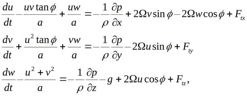

2. Gravitational force

      M – mass of the Earth, m - mass of the elementary volume of air, , gravitational
                                      force:

                                                          .

 In dynamic meteorlogy and oceanology reference frame is attached to the planetary
  surface. When a is the mean radius of the Earth (mean sea level), neglecting small
deflections of the planetary shape from spherical, we may introduce vertical coordinate
                       z and             Then we may introduce:

                                                      ,

 where                        is gravitational force at the sea level. In meteorology and

         ocaenology             , and with a good approximation               .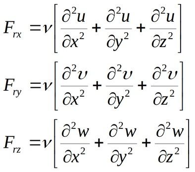

3. Friction and viscosoty.
We know that in many cases friction between the atmosphere and the earth surface
cannot be neglected. A kind of friction (viscosity) results from molecular structure of air
and water.. Consider elementary volume of air                 :

     When the shear stress in direction    acting in the middle of the volume is     , then
the shear stress at the upper side of the volume can be written as:

                                                      ,

                               while at the bottom side it is:

                                                          .

Total force acting at the volume through its top and bottom is:

                                                                     .

 Thus, friction per unit mass of fluid due to vertical gradient of       - velocity component
                                     can be written as:

                     (since                 and                          ).

For              the above can be written as:

                                                      ,

where            is kinematic viscosity, for air                  .

Considering all three directions we may write:

For the atmosphere, at heights below 100 km kinematic viscosity       is so small that can
be neglected except for a few cm thick layer close to the surface. The same is true for
water.
The effective friction in the atmosphere and ocean results from bulk momentum
transport by turbulence and convection, not (directly) by molecular viscosity. ,

From the practical perspective often (not always!!!) eddy viscosity can be introduced to
describe friction in turbulent environment. Unfortunately, eddy viscosity is property of
particular flow, not of the fluid.

4. Apparent forces: centrifugal force.
    Consider air parcel of mass     , rotating along circle of radius    with the
angular velocity    . Consider external reference frame. In order to calculate
acceleration
we take velocity difference           , during time      in which parcel changes direction
by the angle of      .

       is also an angle between          and           , and          is just           .

In the limit         ,        is directed towards axis of rotation:

                                                         ,

but            and             , so               : acceleration is directed towards axis of

rotation. In the rotating reference frame the apparent force – centrifugal force is needed
to explain parcel motion.

In case of the Earth, rotating with angular velocity         (               rad s-1) and
distance of a given location from the axis of rotation equal         ,

the apparent force acting on the parcel of air is equal to       *       .

This force, from the point of view of the observer at the earth's surface can be added to
the gravitational force resulting in ….

                            effective gravitational force - gravity.

4a. effective gravitational force – gravity.

    Acceleration due to this force is described as :                   .

      Gravitational force is directed toward the center of the Earth, while centrifugal force
is directed outside from the axis of rotation. In effect, everywhere between the Poles
and the Equator gravity does not point toward the center of the earth and the shape of
the Earth resembles more ellipsoid than a ball. On the other hand, gravity is always
perpendicular to the Earth's surface and deflection from a spherical shape is small:
difference between polar and equatorial radii is ~21 km.

Gravity acceleration can be described in terms of potential of certain function

                              called GEOPOTENTIAL.

     Since            , where          , then               and               .

For value of geopotential equal to zero at zero height, geopotential        at height
          is equal to the work needed to lift unit mass from the mean sea level
                                to the height

                                         z

                                    Φ =∫ gdz     .
                                         0

5. Coriolis force.

     Consider air parcel of unit mass moving towards east. Effective rotation of a sum
of the rotation of the Earth and motion with respect to the surface of the Earth. When

      is the Earth's angular velocity,     describes distance from the axis of rotation
and        is the eastwards velocity component relative to the surface then:

                                                                .

First term in the RHS of the equation is the centrifugal acceleration due to Earth's
 rotation (part of gravity force), second term           represents Coriolis acceleration,
 third term, centripetal acceleration, for typical atmospheric motions is negligible, since
                                                     .
Notice that Coriolis acceleration due to west-east motion with respect to the surface of
the planet can be decomposed into north-east :

                                       ,and vertical :

                                     components.
Here            denote eastward, northward and upward velocity components,             is
latitude and index      notes Coriolis effect.

Formally Coriolis force (acceleration) can be introduced in the following way.

We know that total derivative of any vector in the rotating frame is:

and in inertial reference frame Newton’s second law of motion may be written
symbolically as:

where index “a” stays for absolute.
In order to transform this expression to rotating coordinates, one must first find a
relationship between Ua and the velocity relative to the rotating system U:

which gives:

Taking total derivative one obtains:

Substituting from Ua into the right-hand side one gets:

where Ω is constant and R is a vector perpendicular to the axis of rotation, with
magnitude equal to the distance to the axis of rotation. We used identity:

If we assume that the only real forces acting on the atmosphere are the pressure
gradient force, gravitation, and friction, we can rewrite Newton’s second law with the aid
of the above as:

                                                             ,

 here        is friction and we combined gravitation and centrifugal forces into gravity .

5. Equation of motion.

The above form of the equation of motion is widely used in geophysical fluid dynamics.
It is often written in the Cartesian reference frame attached to the Earths surface. Axes
are along          , where      is longitude,     is latitude, and      is vertical.

In such reference frame components are:

6. Scale analysis: synoptic motions in mid-latitudes.

We perform scaling the equations of motion in order to determine whether some terms
in the equations are negligible for motions of particular concern. Elimination of terms on
scaling considerations not only has the advantage of simplifying the mathematics, but
as shown later the elimination of small terms in some cases has the very important
property of completely eliminating or filtering an unwanted type of motion.

The complete equations of motion describe all types and scales of geophysical flows.
Sound waves, for example, are a perfectly valid class of solutions to these equations.
However, sound waves are of negligible importance in dynamical meteorology or
oceanology. Therefore, it will be a distinct advantage if, as turns out to be true, we can
neglect the terms that lead to the production of sound waves and filter out this
unwanted class of motions.

In order to simplify equations for synoptic scale motions, we define the following
characteristic scales of the field variables based on observed values for midlatitude
synoptic systems.
                                      m s-1 – horizontal velocity scale
                                    cm s-1 – vertical velocity scale
                                     m – length scale - 1000 km
                                       m – depth scale - 10 km
                                   m2s-2 – pressure fluctuations in horizontal
                                                s – time scale

Horizontal pressure fluctuations         are normalized by density       , to have dcale
valid through troposphere depth, since both :          and       decrease (exponentially)
with height. Additionally,          is in the units of geopotential.
Other important scales

           f =2 Ω sin( φ )≈1.6∗10− 4 ∼10−4 s-1 – Coriolis parameter at midlatitudes
                                               5
                        a=6400[km]∼10 m – radius of the Earth

is a time to travel distance       with velocity       .

The resulting material derivative of such motions scales as                 .

 Scale analysis of horizontal components of the momentum equation:

                A      B         C     D        E          F        G
          X:

          Y:

           S:        f 0U

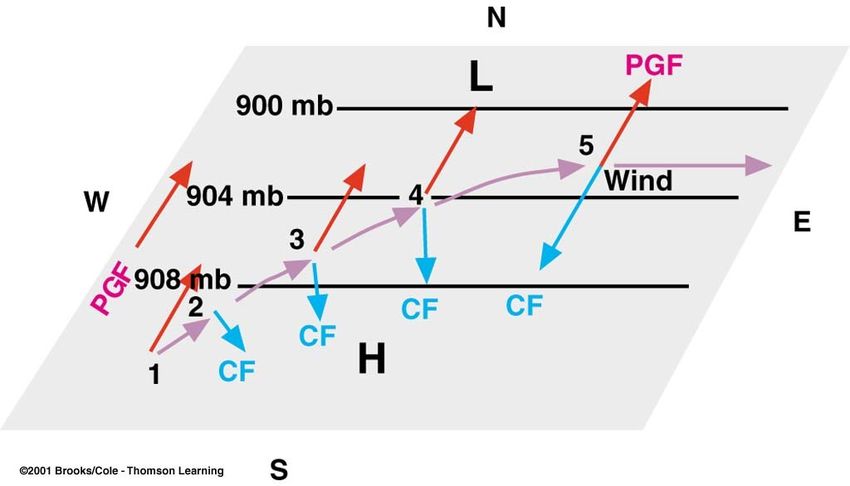
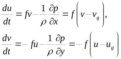
          W:

Geostrophic approximation

          first approximation of the above scale analysis results in:
                                     ,            ,

               where                is Coriolis parameter.

Flow resulting from balance between Coriolis and pressure gradient forces
                          is called geostrophic wind defined as:

                                            .

In mid-latitudes geostrophic wind differs from the actual wind for 10-15%.

Prognostic approximation, Rossby’ number.

  The next approximation of equations of motion takes the form:

This approximation is called “quasi-geostrophic” or “prognostic”

   Ratio of the acceleration in the above equation to Coriolis is:

                                        ,

                          Rossby number.

Scale analysis of the vertical component:

Because pressure decreases by about an order of magnitude from the ground to the
tropopause, the vertical pressure gradient may be scaled by P0 /H , where P0 is the
surface pressure and H is the depth of the troposphere.

The scaling indicates that to a high degree of accuracy the pressure field is in
hydrostatic equilibrium; that is, the pressure at any point is simply equal to the weight
of a unit cross-section column of air above that point.

The above analysis of the vertical momentum equation is, however, somewhat
misleading. It is not sufficient to show merely that the vertical acceleration is small
compared to g. Because only that part of the pressure field that varies horizontally is
directly coupled to the horizontal velocity field, it is actually necessary to show that the
horizontally varying pressure component is itself in hydrostatic equilibrium with the
horizontally varying density field.

Let's define standard pressure p0(z), which is the horizontally averaged pressure at
each height, and a corresponding standard density ρ0(z), which are in exact hydrostatic
balance:

Let's write:

where p' and ρ' are deviations from the standard values of pressure and density. For an
atmosphere at rest, p' and ρ' would thus be zero. Then, assuming ρ'/ρ0

For synoptic scale motions

which can be compared with terms in Table 2.
To a very good approximation the perturbation pressure field is in hydrostatic
equilibrium with the perturbation density field and:

Therefore, for synoptic scale motions, vertical accelerations are negligible.

This leads to the approximation in which the vertical velocity cannot be determined from
the vertical momentum equation, it has to be deduced indirectly!

However, fact that pressure is related to density with hydrostatic relation:

allows usage of pressure as vertical coordinate!

Balanced flows.
            Natural Coordinates
                                  The natural coordinate system is defined by the
                                  orthogonal set of unit vectors t, n, and k.
                                  Unit vector t is oriented parallel to the horizontal
                                  velocity at each point;
                                  unit vector n is normal to the horizontal velocity
                                  and is oriented so that it is positive to the left of
                                  the flow direction;
                                  unit vector k is directed vertically upward.
                                  In this system the horizontal velocity may be
                                  written V = V t where V , the horizontal speed, is a
                                  non-negative scalar defined by V ≡ Ds/Dt,
                                  s(x, y, t) is the distance along the curve followed
                                  by a parcel moving in the horizontal plane.
                                  Then:

and

R is the radius of curvature following the parcel motion, by convention, R is positive
when the center of curvature is in the positive n direction. Thus, for R > 0, the air turn
toward the left following the motion, and for R < 0 toward the right.

We may calculate:

The Coriolis force always acts normal to the direction of motion:

and pressure gradient can be expresses as:

in natural coordinates.

The horizontal momentum equation can be expanded into components :

For motion parallel to the geopotential height contours, ∂Φ/∂s = 0 and the speed is
constant. When the geopotential gradient (normal to the direction of motion) is constant
the above implies constant radius trajectory at given latitude.
In that case the flow can be classified into several simple categories.

  1. Geostrophic Flow
Flow in a straight line (R → ± ∞)
parallel to height contours.

2. Inertial Flow
     For uniform geopotential on an isobaric surface the horizontal pressure gradient
     vanishes, and a balance between Coriolis force and centrifugal force exists:

The above gives:

Fluid air parcels follow circular paths in an anticyclonic sense. The period of this
oscillation is:

Because both the Coriolis force and the centrifugal force due to the relative motion are
caused by inertia of the fluid, this type of motion is traditionally referred to as an inertial
oscillation, and the circle of radius |R| is called the inertia circle.

Notice that inertial oscillations are important for the ocean surface!!!!!

A drifting buoy set in motion by strong westerly winds in the Baltic Sea in July 1969.
When the wind has decreased the uppermost water layers of the oceans tend to follow
approximately inertia circles due to the Coriolis effect. This is reflected in the motions of
drifting buoys. In the case there are steady ocean currents the trajectories will become
cycloides. The inertia circles are not eddies; a set of buoys close to each other would
be co-moving, rather than revolve around each other..

Consider inertial oscillation visualizer at:
http://oceanmotion.org/html/resources/coriolis.htm

4. Cyclostrophic Flow
     If the horizontal scale of a flow is small enough, the Coriolis force may be
     neglected in compared to the pressure gradient force and the centrifugal force
     and:

This flow can be either cyclonic or anticyclonic.
The cyclostrophic balance approximation is valid provided that the ratio of the
centrifugal force to the Coriolis force V /(fR) large. This ratio is equivalent to the Rossby
number
Consider a typical tornado of the tangential velocity of 30 ms−1 at a distance of 300 m
from the center of the vortex. Assuming that f =10−4 s−1 , the Rossby number is :

                                     Ro = V /|f R| ≈ 103.

4. The Gradient Wind Approximation
     Horizontal frictionless flow that is parallel to the height contours so that the
     tangential acceleration vanishes (DV /Dt = 0) is called gradient flow. Gradient flow
     is a three-way balance among the Coriolis force, the centrifugal force, and the
     horizontal pressure gradient force:

Solving the balance one gets:

Not all the mathematically possible roots of the above correspond to physically possible
solutions, as it is required that V be real and non-negative. The various roots are
classified according to the signs of R and ∂ /∂n in order to isolate the physically
meaningful solutions.