Ecotone response to climatic variability depends on stress gradient interactions
←
→
Page content transcription
If your browser does not render page correctly, please read the page content below
-

Ecotone response to climatic variability depends
on stress gradient interactions
Malanson, George P; Resler, Lynn M; Tomback, Diana F
https://iro.uiowa.edu/discovery/delivery/01IOWA_INST:ResearchRepository/12675005440002771?l#13675073420002771

Malanson, G. P., Resler, L. M., & Tomback, D. F. (2017). Ecotone response to climatic variability depends on
stress gradient interactions. Climate Change Responses, 4. https://doi.org/10.1186/s40665-017-0029-4
Document Version: Published (Version of record)

DOI: https://doi.org/10.1186/s40665-017-0029-4

https://iro.uiowa.edu
CC BY V4.0
Copyright © 2017 The Author(s)
Downloaded on 2021/10/16 16:33:18 -0500

-
Malanson et al. Climate Change Responses (2017) 4:1
DOI 10.1186/s40665-017-0029-4

 RESEARCH                                                                                                                                        Open Access

Ecotone response to climatic variability
depends on stress gradient interactions
George P. Malanson1, Lynn M. Resler2 and Diana F. Tomback3*

  Abstract
  Background: Variability added to directional climate change could have consequences for ecotone community
  responses, or positive and negative variations could balance. The response will depend on interactions among
  individuals along environmental gradients, further affected by stress gradient effects.
  Methods: Two instantiations of the stress gradient hypothesis, simple stress and a size-mediated model, are
  represented in a spatially explicit agent based simulation of an ecotone derived from observations of Abies
  lasiocarpa, Picea engelmannii, and Pinus albicaulis in the northern Rocky Mountains. The simple model has two
  hierarchically competitive species on a single environmental gradient. The environment undergoes progressive
  climate change and increases in variability. Because the size model includes system memory, it is expected to
  buffer the effects of extreme events.
  Results: The interactions included in both models of the stress gradient hypothesis similarly reduce the effects of
  increasing climatic variability. With climate amelioration, the spatial pattern at the ecotone shows an advance of both
  species into what had been a higher stress area, but with less density when variation increases. In the size-mediated
  model the competitive species advances farther along the stress gradient at the expense of the second species. The
  memory embedded in the size-mediated model does not appear to buffer extreme events because the interactions
  between the two species within their shifting ecotone determine the outcomes.
  Conclusions: Ecotone responses are determined by the differences in slopes of the species response to the
  environment near their point of intersection and further changed by whether neighbor interactions are competitive.
  Interactions are more diverse and more interwoven than previously conceived, and their quantification will be
  necessary to move beyond simplistic species distribution models.
  Keywords: Agent based model, Competition, Ecotone, Extinction, Facilitation, Simulation, Variability

Background                                                                            new insights [7] necessitating 1) the need to incorporate
As the global climate changes, shifts in climatic variabil-                           interactions among organisms in species distribution
ity, including extremes, could have ecological conse-                                 models, e.g. [8], and 2) recognition of climatic variation
quences at least as great as would result from changes in                             [8]. We aim to examine how different hypothesized
mean temperature and precipitation [1–3]. Thus, the                                   modes of plant interaction alter ecological response to
ecological impacts of climatic variability requires re-                               changing climatic variability. We use a spatially explicit,
search [4, 5], specifically on how climate variability will                           two-species, agent-based model (derived from an earlier
affect population processes, and how to apply basic eco-                              model of alpine treeline in the Rocky Mountains, USA)
logical theory to understand community responses to                                   with contrasting gradients of change in the relative
climate change. Current theory is rooted in ideas on fre-                             strength of competition and facilitation to simulate re-
quency dependent population processes such as compe-                                  sponses of an ecotone to climatic variability.
tition [6], but ideas based on facilitation may provide

* Correspondence: george-malanson@uiowa.edu                                           Climatic variability
3
 Department of Integrative Biology, CB 171, University of Colorado Denver,
P.O. Box 173364, Denver, CO 80217, USA
                                                                                      Work on climatic variability has indicated that anomal-
Full list of author information is available at the end of the article                ies (in climatology, the difference from average) in one
                                        © The Author(s). 2017 Open Access This article is distributed under the terms of the Creative Commons Attribution 4.0
                                        International License (http://creativecommons.org/licenses/by/4.0/), which permits unrestricted use, distribution, and
                                        reproduction in any medium, provided you give appropriate credit to the original author(s) and the source, provide a link to
                                        the Creative Commons license, and indicate if changes were made. The Creative Commons Public Domain Dedication waiver
                                        (http://creativecommons.org/publicdomain/zero/1.0/) applies to the data made available in this article, unless otherwise stated.
Malanson et al. Climate Change Responses (2017) 4:1 Page 2 of 8
direction could be balanced by anomalies in the other (high density can also result in competition for soil re-
direction. However, the potential ecological importance sources, including water); single trees may have different
of climatic variability has also been recognized. For ex- effects [26]. A variety of interactions are being explored
ample, extreme events change high or low temperature as limits on treeline upslope advance in response to cli-
regimes and exacerbate moisture limitations from a state mate change [27].
of stress to one of disturbance, because their physio- At treeline, the extreme limit of the stress gradient for
logical effects change from reduced productivity to mor- trees, the most exposed individuals can benefit most from
tality. Kayler et al. have called for inclusion of variation positive feedback. Moreover, the positive feedbacks at the
in experimental approaches to ecological response [9]. edge may be critical to tree recruitment, whereas the
Introducing variability in rain-exclusion or—addition ex- negative feedbacks may be limited by the small size of in-
periments should be straightforward, but otherwise well- dividuals ([28]. This size dependence is part of the ration-
developed experiments sometimes do not explore this ale for our size gradient model, and incorporating relative
factor (or have been too short). Where variation has sizes of interacting plants and the resulting effects more
been introduced, experiments show the effects of func- be a more realistic portrayal of community processes.
tional diversity [10]. From simulations, Malanson [11]
reported that competition affected population responses Rationale
to increasing variability more than biological (i.e., gen- We use a corollary to the SGH, a relative size gradient
etic) or spatial constraints. (RSG) model [29], which incorporates a more mechanistic
feedback between the abiotic and biotic components of the
Ecotones and facilitation environment. The SGH holds that competition will
Ecotones have been a focus for examining ecological re- decrease and facilitation increase along a gradient of in-
sponse to climate change [12]. For treeline ecotones in creasing environmental stress [30, 31] (. The particular en-
particular, research has focused on positive interactions vironmental processes or gradients through which
among individuals and has downplayed competition interactions operate are varied and potentially combined
[13]. Given the observation of ecotone boundaries that [32]. The RSG model mediates the SGH by providing a
were abrupt relative to the environmental gradient in more direct mechanism for a change in net interaction be-
which they were observed, the positive feedback switch tween positive and negative and a feedback through growth
hypothesis [14] became the dominant explanation; e.g., rates. Malanson and Resler found that the RSG produces
[15–17]. This emphasis on facilitation at ecotones such similar patterns of response to climate change in simula-
as alpine treeline became blended with the stress gradi- tions [29]; the reason is that in the area of high stress the
ent hypothesis (SGH) [18, 19] (which is flexible in the largest plants are never so much larger than the smaller
details depending on the stressor; alpine treelines can be that they become competitors instead of facilitators.
locally water stressed within a broader scale stress of The response of alpine treeline to increasing variability
heat deficit [13]). de Dios et al. showed how a temporal with climate change could depend on whether the feed-
switch in interaction could be a factor in ecotone re- back process is a direct function of level of environmental
sponse to climate change [20]. Rates of response to cli- stress (the classic SGH) or mediated by plant size, as we
mate change may also be tied to species interactions suggest. The SGH embodies a direct effect of plants on
[21]. Moreover, treeline dynamics have been shown to the local environment, modifying the stress on other
respond to interannual climatic variability [22]. plants. The size gradient model builds memory into the
At alpine treeline ecotones the population dynamics system. The sizes of plants can increase only incrementally
and spatial distributions of conifers are affected by both (but can decrease drastically with mortality) so the effects
negative and positive feedbacks within their community. of climatic variability are buffered by the existing size of
The canopy reduces wind, which in turn reduces evapo- plants. We hypothesize that a stress gradient system will
transpirative stress in its neighborhood, captures snow be more sensitive to increasing variation in the climate
that becomes late-summer soil moisture in an otherwise than would a size gradient system because the feedback
dry environment, and increases the accumulation of fine within the latter will change slowly. The addition of a size
sediment and organic matter in the soil [13, 23]. Further, gradient model contributes to an effort to include a variety
the canopy reduces the impact of UV radiation and of of plant-plant interactions in the study of species range
night sky exposure and cold temperature photoinhibi- limits with climate change, e.g., [33].
tion in its neighborhood [24]. Conversely, the shade cast To examine how interactions mediate variability, we
by closed canopies (especially in krummholz) limits light model the ecotone dynamics between two populations
availability, and perhaps more importantly, maintains by simulating the effects of a changing climate with
colder soil temperatures under the canopy, which may increasing variability on a spatially explicit environmen-
be the limiting factor for treelines at global scale [25] tal gradient. We simulate population dynamics andMalanson et al. Climate Change Responses (2017) 4:1 Page 3 of 8
extinctions, which are likely to respond to variability of reproduction, the amount of growth, and the prob-
[34]; although demographic stochasticity is included, we ability of mortality.
do not manipulate it. Ecotones may be revealing indica-
tors of the consequences of climate change. Alpine tree- Model design
lines are simple in that they support few tree species We use a spatially explicit agent based model created in
(often 1–2), and the environmental gradient, from the Netlogo [40], Additional file 1. The model is based on a
“plant’s eye view” (sensu Harper, p 706 [35]), is relatively grid of 1000 x 50 cells, wrapped as a cylinder to elimin-
simple if the decline in tree size and density is assumed ate edge effects. The plant’s-eye-view of the environment
to be indicative. We acknowledge that the model is so is defined by responses of two species (SpS, for specialist
simplified that it will not differentiate all of the specific and SpG for generalist, subscript s) on the long axis of
processes; cf. [36]. Körner recently emphasized the role the grid set as hierarchical Gaussian curves, Eys, 1-0
of size on feedbacks, but did not lay out a complete across the rows (subscript y) as shown in Fig. 1 (cf. [41]).
framework for the role of size that would capture effects This approach collapses the various dimensions of niche
of neighbors and water limitations [28]. Although this is to a single gradient appropriate for a simple exploratory
the type of two-species model that is common in theor- model. The responses in this model are relative but are
etical ecology, it is based on observations of Pinus albi- based on observations of Abies lasiocarpa and Picea
caulis, Abies lasiocarpa, and Picea engelmannii. engelmannii, for SpS, and Pinus albicaulis, for SpG, at
Observations at alpine treeline ecotones in the northern alpine treeline in western North America (see [42]). P.
Rocky Mountains indicate that P. albicaulis is a pioneer albicaulis is a pioneer, keystone, and foundational spe-
species, able to establish in open areas where it then cies at alpine treeline; it is able to reproduce in high-
provides facilitation for the establishment of A. lasio- stress environments without neighbor facilitation, and it
carpa and P. engelmannii [37]. The mechanistic nature grows slowly. A. lasiocarpa and P. engelmanni often es-
of facilitation indicates that size is likely to be relevant tablish next to extant P. albicaulis and have somewhat
[26], and neighbors affect size [38]. higher growth rates. Information on survivorship is
We hypothesize that the simulation of outcomes in sparse because treeline sites are relatively new (since the
populations, extinctions, and spatial outcomes will differ Little Ice Age in the Rocky Mountains [43]) but the ages
among the models of no interaction (none), SGH inter- of P. albicaulis are much greater than any of the other
action (stress), and the size model (size) of interaction. two species at sites where we have examined tree rings
Our expectation is that stress gradient and size gradient (e.g., [44]). Although the gradient is smooth, the feed-
feedback models will buffer the response to climatic back that is simulated creates clumped patterns of spe-
variability so that the relative sensitivity would be: cies occurrences. Feedback is likely to be more
none > stress > size. important in the spatial heterogeneity of factors such
as microclimate or soils than are purely abiotic pro-
Methods cesses [45].
Conceptual model Each cell of the grid can be occupied by one individ-
We use a simplistic model to elucidate the effects of ual, and to initialize model runs, all cells are occupied by
variability for the types of environmental gradients and an individual j, at a random size between 1 and 100, with
species niche dimensions envisioned for ecotones, spe- a probability proportional to Eys. The dynamics of the
cifically for hierarchical competition and the SGH. We
use an approach that eliminates the need to know the
response of a particular system to specific changes in cli-
mate. Instead, we consider the plant’s-eye-view by vary-
ing habitat quality as a composite parameter and change
it through time with and without increasing variability
during a period of improving habitat quality.
The model assumes that interactions among plants are
based on the relative size of the focal individual and the
summed sizes of its neighbors and that this interaction
intensity is a multiplier the habitat quality, which is 1 for facilitative effects; the
range is from 0.5 to 2; [39] for details. The model com-
putes the habitat quality given an initial environmental Fig. 1 The species-specific habitat quality assigned to each row of
the grid. This value is used in multiplier to compute the probability
gradient multiplied by the interaction intensity. This
of recruitment and mortality and the amount of growth
habitat quality is then used to determine the probabilityMalanson et al. Climate Change Responses (2017) 4:1 Page 4 of 8
population are simulated over 400 iterations of recruit- PðM1 Þ ¼ 1 − :5 I Ey1
ment, growth, and death as Monte Carlo processes with
treatments implemented in the last 100 iterations. Al- PðM2 Þ ¼ 1 − :4 I Ey2
though the initial size distribution is random rather than
realistic, age structure develops during the initial 300 it- The maxima are set at half of the maxima for Eys (1.0
erations before treatments begin. and 0.8) based on the logic that once established mortal-
The stress gradient version is computed as a logarith- ity is relatively rare.
mic increase in interaction intensity with the number of
neighbors: multiplied by a gradient from 0.5 to 2 across Model runs
the length of the grid: To represent climate change, the value of Eys is reset to
Ey-1s in iterations 301–400. Eys increases; the climate
d ¼ number of neighbors
ameliorates in the plant’s-eye-view. Iterations 1–300 with
Istress ¼ :26 þ :333 ln d 2 – 1:5Ey Eys constant allow all relevant variables to equilibrate.
Climatic variability is created by multiplying the values
The size gradient version is for all cells in every year by a random number drawn
from a normal distribution with a mean of 1 and a
d ¼ Sn =Sf
standard deviation of 0.25. We use 0.25 based on the
Isize jd < 33:333 ¼ 1 þ :03d standard deviation of standardized tree-ring widths re-
corded for a > 400 year-old stand of alpine larch at tree-
Isize jd > 33:333 ¼ 3:25 − :0375d
line in Glacier National Park, which range from 0.22 to
where Sn is the sum of the sizes of the eight neighbors 0.25 (personal communication, Greg Pederson); com-
and Sf is the size of the focal individual; for empty cells parison of the two values has revealed much higher ex-
the intensity for recruitment is calculated with Sf = 1 tinction rates for 0.25 when the multiplier doubled over
interaction intensities less than 0.5 or greater than 2 are 200 year [11]. We increase the multiplier to 1.5 over 100
reset to these limits (Fig. 1). A logarithmic form was year, after which it again becomes constant to represent
chosen to give most weight to the first neighbor; cf. [29, a new climatic equilibrium. With the multiplier Eys is
36]. While it would seem that the model would be sensi- constrained to not exceed 1.0 or 0.8 for SpS and SpG,
tive to relative size at which competition begins to out- respectively.
weigh facilitation (here at 10 times, with competition We present the results of six simulations, but we show
reaching its limit at 30), trials with these points set at 3/ the differences between scenarios with constant and with
10 and 33.33/100 produce quantitatively similar results. increasing climatic variability for simulations with no
Although the stress gradient is linear with the environ- feedback, with the stress gradient feedback, and for the
ment, spatial patterns develop because of the density of size gradient feedback. The metrics of analysis here are
neighbors, especially at the treeline. the differences in the population sizes of SpS and SpG
Recruitment for SpS and SpG occurs on cells with between the climatic representations averaged from 100
probability a function of the size of their extant popula- replicate runs, and the proportion of those runs that end
tion relative to the size of the grid and the environment in extinction for either species (extinction/200); simula-
of the row: tion runs in which extinction occurred during the first
20 iterations, prior to equilibration of population sizes,
PðR1 Þ ¼ rN I Ey1 were discarded and replaced.
PðR2 Þ ¼ rN I Ey2
Results
where N is the current population and r is 0.00001 or Even before climate change begins in the simulations,
0.000008 based on the size of the grid, so that the maxima the effect of feedbacks on response to variation becomes
would be with rN = 1.0 or 0.64 for SpS and SpG, respect- evident (Table 1A). In terms of overall population num-
ively. SpG can establish only on empty cells whereas SpS bers, the feedbacks are able to buffer the population re-
can replace SpG but with its recruitment rate halved. Re- sponses to increasing variability. The small difference
cruitment parameters are chosen to reduce dimensionality between the stress and size gradient models depends on
by setting them to allow replacement recruitment in a the species.
hypothetical open, ideal environment. Because of the feed- With climate change and increasing variability, how-
backs, recruitment in the neighborhood of extant individ- ever, effects are more pronounced (Table 1B). Rather
uals is more common in the treeline area. than clearly buffering the population responses to in-
SpS has a higher mortality rate than SpG to match its creasing variability as expected, the simulation repre-
higher reproductive rate: senting the size gradient hypothesis had populationMalanson et al. Climate Change Responses (2017) 4:1 Page 5 of 8
Table 1 Percent difference in each population for the two model
species between scenarios with and without climatic variation for
a control with no feedback and the stress and relative size
gradient models at two times in the simulations runs
Models: None Stress Size
A
SpS −3.5 1.0 −0.4
SpG −2.6 −2.0 −1.0
B
SpS −17 −26 −18
SpG −33 −11 −42
A) before climate change (at iteration 300), and B) after climate change
(iteration 400) Fig. 2 Absolute difference in sizes from the populations at iteration
200 for the two species in the three feedback models during the
iterations of increasing climatic variation (301–400)
changes similar to the no feedback scenario especially
for SpS, while for SpG the size gradient version had
greater population loss with climate change and increas- increasing variability as it is for SpG. In the size gradient
ing variability and the stress gradient version lost least. model SpS is able to advance further into the high stress
The stress gradient hypothesis is able to minimize the zone, and without variability SpG has a denser population
impact of variability on SpG by increasing the intensity (fewer empty cells in this area), but with increasing vari-
and effect of facilitation in the area of the grid that was ability SpG is less dense than in any other case.
previously empty, but with climate change becomes hab- Before climate change begins in the simulations, differ-
itable. However, because competition dominates in the ences have developed among the three models (Fig. 3
area occupied preferentially by SpS, i.e. the better habitat A,D,G; no feedback, stress gradient, and size gradient).
quality, in the stress gradient simulations, its population Relative to no feedback, the stress gradient has the eco-
is more strongly affected by increasing variability than tone between SpS and SpG in about the same place on
either the no feedback or size gradient versions. The size the grid but the transition zone is longer (Fig. 3 B,E).
gradient hypothesis turns out to be sensitive to variation. Additionally, SpG is denser farther upslope. With the
In the high stress part of the gradient, the effects of size size gradient model the transition zone is farther up-
are limited because growth rates are low and sizes re- slope, the area of SpG dominance is about the same, but
main small. Relative to the amplitude of climatic vari- its density is similar to the case with no feedback (less
ation, the effects of feedback remain small in this area. than for the stress gradient) (Fig. 3 C,I).
In proportional change, the stress gradient representa-
tion buffered the responses of the populations more than
that of the size gradient hypothesis, contrary to our ex- Discussion
pectations. However, in absolute terms this difference is The relative size gradient model assumes that neighbor
because the size gradient maintained larger populations interactions affecting a focal individual reach a positive
than did the stress gradient as simulated (Fig. 2). With peak when the neighbors are somewhat larger, but be-
the size gradient the population of SpS is higher before come negative when much larger. It is a more mechanis-
climate change and both populations are higher after it. tic portrayal of feedbacks on an environmental gradient
While the stress gradient, in theory, could allow individ- than the SGH, because of its direct tie between the
uals to develop larger populations in the high stress por- resulting size and the mechanism of growth. However, in
tion of the gradient, any facilitation depends on multiple observed effects it is modestly different from simulations
rare recruitments, and with climatic variability rare indi- based on the SGH. For both models the differences from
viduals are eliminated before they are joined by others. the no-feedback simulations are qualitatively similar in
With respect to the probability of extinction, simula- population responses and spatial patterns.
tions indicated that the stress and size gradient models
showed little difference in effect (Table 2). A visualization Table 2 The percent of simulation runs in which a species went
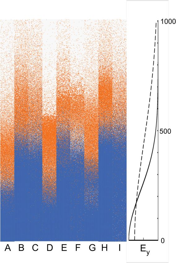
helps to interpret the model outcomes (Fig. 3). With cli- extinct (N = no climatic variability; V = climatic variability)
mate change (B, C, E, F, H, I) the populations advance into NoneN NoneV StressN StressV SizeN SizeV
the higher stress area. With increasing variability, the pop-
Sp1 0 10 3 11 1 12
ulations are not as dense as the simulations with no vari-
Sp2 1 10 3 12 1 12
ability. The advance for SpS is not as retarded by theMalanson et al. Climate Change Responses (2017) 4:1 Page 6 of 8
intraspecific and interspecific interactions in the model, the
latter occur. Scramble competition occurs in the ecotone
between SpS and SpG regardless of whether the individual
interactions are positive or negative. Second, undifferenti-
ated individual interactions can be based on location.
In the stress gradient model, SpS is confined to the area
that experiences competition because the environment is
less stressful. As the environment improves, SpS moves
upslope, but still primarily experiences competition
among individuals. With increasing climatic variability,
improvements in the environment are accompanied by in-
creases in competition so SpS is not able to take advantage
of those positive anomalies. SpG is less affected because it
has open area to advance into when the environment im-
proves and it is experiencing modest facilitation which is
only increased when the anomalies are negative.
In the size gradient model, SpG is able to take advan-
tage of the improving environment without climatic
variability by moving upslope into previously unoccupied
area. With increasing variability, the dependence on size
buffers its response to the favorable anomalies because
there is a biological limit to improvement (the response
is never greater than 0.7). A negative anomaly that re-
sults in mortality is not easily reversed in a subsequent
year. Thus the net outcome is highest sensitivity for the
scenario we predicted would be lowest.
The mode of interaction does mediate the effects of in-
creasing climatic variability in our model, but not as ex-
Fig. 3 Comparison of the spatial patterns across the rows of the grid pected. The size gradient model is more sensitive to
(graph Ey corresponds to Fig. 1) produced by the simulations for SpS
increasing climatic variability because of the way that the
(blue) and SpG (orange). ABC, DEF, and GEH use no feedbacks or those
for the stress and size models, respectively. The patterns are shown boundary and interactions between the two species re-
prior to beginning climate change in the simulations (iteration 300: A, spond. The interaction at the boundary is affected by how
D, G) and for after climate change (iteration 400) without increasing species respond to the environmental gradient at the point
variability (B, E, H) and with increasing variability (C, F, I). Base variance where they intersect in Fig. 1; cf. [11, 40]. Climatic vari-
has the standard deviation of 0.22
ability should have the greatest effect on SpS because its
response curve is steeper at the crossover point. This is
While we had expected that the size gradient model also where size differences do not buffer responses be-
would be less sensitive to increasing climatic variability, cause the greatest differences in size of neighbors is in the
sensitivity varied by species. Without any feedback, SpG least stressful part of the gradient where individual sizes
was more sensitive to increasing variability as climate can be large next to newly recruited neighbors.
improved than SpS. Although SpG was able to move up- The size gradient model introduces a specific feedback
slope in both cases, with increasing variability it did not mechanism that allows a change from facilitation to
lead to as many individuals over the entire gradient and competition as the relative sizes of the plants diverge.
so appears to be less dense spatially. With the stress gra- This model introduces a single functional trait, but from
dient model of feedback, SpS is more sensitive than a different perspective than most of the functional traits
SpG. The increasing climatic variability restricts the up- commonly discussed for plant species. Most work on
slope advance of both species, but to a greater extent for functional traits is about indicators of functions within
SpS, leaving a less dense ecotone with a preponderance individuals [46]. Our perspective comes from the conse-
of SpG. The effects switch in the size gradient model. quences of altering the abiotic environment of a neigh-
Although the upslope advance is similar with and with- borhood. Some commonly used traits, such as canopy
out increasing climatic variability, in both cases the dis- height, can have either individual or neighborhood func-
tribution of SpG is less dense. tions, but differentiating the two will be important in
The effects of increasing climatic variability depend on assessing their role in plant community response to
interactions. First, although we do not differentiate climate change [8].Malanson et al. Climate Change Responses (2017) 4:1 Page 7 of 8
Conclusions Availability of data and material
The consequences of increasing climatic variability as The Netlogo simulation code is available in the Netlogo community models
archive at: https://ccl.northwestern.edu/netlogo/models/community/
climate changes depend on the environmental gradient index.cgi. Search MalansonReslerTomback.
as experienced from the plant’s-eye-view, which is af-
fected by interactions with neighbors. At ecotones, this Authors’ contributions
plant’s-eye-view determines the transition in dominance All authors contributed substantially to the ideas presented in this paper. GPM
led the model development phase. GPM and LRM led the writing, and all
from one species or vegetation type to another. In our edited the manuscript. All authors read and approved the final manuscript.
model this interaction is determined by the differences
in slopes of the species response to the environment Competing interests
near their point of intersection as represented in Fig. 1 The authors declare that they have no competing interests.
but further changed by whether neighbor interactions
Consent for publication
are competitive or facilitative according to the SGH. NA.
Broad representation of species niche based on pres-
ence without quantified interactions will be inadequate Ethics approval and consent to participate
for assessing their response to climate change. While NA.
long recognized [47] but still often ignored, inclusion of Author details
plant-plant interactions is necessary to model the transi- 1
Department of Geographical & Sustainability Sciences, University of Iowa,
ent responses of ecosystems to climate change (along Iowa City, IA 52242, USA. 2Department of Geography, Virginia Tech,
Blacksburg, VA 24061, USA. 3Department of Integrative Biology, CB 171,
with dispersal and fragmentation). We now see that in- University of Colorado Denver, P.O. Box 173364, Denver, CO 80217, USA.
teractions are even more diverse, more interwoven, and
more important. The plant’s-eye-view will be necessary Received: 27 September 2016 Accepted: 4 January 2017
to move beyond simplistic species distribution models.
For the specific type of ecotones that motivated this References
model, alpine treelines, both variability and the nature of 1. Easterling DR, Meehl GA, Parmesan C, Changnon SA, Karl TR, Mearns LO.
stress gradient interactions will be relevant to their re- Climate extremes: observations, modeling, and impacts. Science. 2000;289:
2068–74.
sponse to climate change. For Pinus albicaulis, instances 2. Helmuth B, Russell BD, Connell SD, Dong Y, Harley CDG, Lima FP, et al.
of dieback as modeled here have been observed in Califor- Beyond long-term averages: making biological sense of a rapidly changing
nia and attributed to water deficit [48]. Inclusion of tem- world. Clim Change Resp. 2014;1:6. doi:10.1186/s40665-014-0006-0.
3. Vasseur DA, DeLong JP, Gilbert B, Greig HS, Harley CDG, McCann KS, et al.
poral autocorrelation of climatic variability is warrented. Increased temperature variation poses a greater risk to species than climate
How individuals and species interact is also likely to affect warming. Proc Roy Soc B. 2014;281:20132612.
the spatial response of the species to climatic change. 4. Smith MD. The ecological role of climate extremes: current understanding
and future prospects. J Ecol. 2011;99:651–5.
Interactions could exacerbate or ameliorate dieback, 5. Reyer CPO, Leuzinger S, Rammig A, Wolf A, Bartholomeus RP, Bonfante A, et
depending on the climatic parameter that drives the al. A plant’s perspective of extremes: terrestrial plant responses to changing
response [37], but general indications of facilitation even climatic variability. Glob Change Biol. 2013;19:75–89.
6. Chesson P. Mechanisms of maintenance of species diversity. Ann Rev Ecol
in dry environments would support an advance of treeline Syst. 2000;31:343–66.
barring the extremes modeled here or exogenous distur- 7. Filazzola A, Lortie CJ. A systematic review and conceptual framework for
bances (fire, pests, disease) not included (cf. [49]). mechanistic pathways of nurse plants. Glob Ecol Biogeogr. 2014;23:1335–45.
8. Heikkinen RK, Luoto M, Virkkala R. Does seasonal fine-tuning of climatic
variables improve the performance of bioclimatic envelope models for
migratory birds? Divers Distr. 2006;12:502–10.
Additional file 9. Kayler ZE, De Boeck HJ, Fatichi S, Grunzweig JM, Merbold L, Beier C, et al.
Experiments to confront the environmental extremes of climate change.
Additional file 1: The Netlogo code for the size gradient model. The Front Ecol Env. 2015;13:219–25.
Netlogo system can be downloaded at https://ccl.northwestern.edu/ 10. Gherardi LA, Sala OE. Enhanced interannual precipitation variability increases
netlogo/. (NLOGO 22 kb) plant functional diversity that in turn ameliorates negative impact on
productivity. Ecol Lett. 2015;18:1293–300.
11. Malanson GP. Interactions and constraints in model species response to
environmental heteroscedasticity. 2016. available online at ir.uiowa.edu.
Abbreviations
12. Kupfer JA, Cairns DM. The suitability of montane ecotones as indicators of
SGH: Stress gradient hypothesis
global climatic change. Prog Phys Geogr. 1996;20:253–72.
13. Malanson GP, Resler LM, Bader MY, Holtmeier F-K, Weiss DJ, Butler DR.
Acknowledgments Mountain treelines: a roadmap for research orientation. Arct Antarct Alp Res.
This material is based upon work while GPM served at the National Science 2011;43:167–77.
Foundation. Any opinion, findings, and conclusions or recommendations 14. Wilson JB, Agnew ADQ. Positive feedback switches in plant communities.
expressed in this material are those of the author and do not necessarily Adv Ecol Res. 1992;23:263–336.
reflect the views of the National Science Foundation. 15. Alftine KJ, Malanson GP. Directional positive feedback and pattern at an
alpine tree line. J Veg Sci. 2004;15:3–12.
16. Bader MY, van Geloof I, Rietkerk M. High solar radiation hinders tree
Funding regeneration above the alpine treeline in northern Ecuador. Plant Ecol.
NA. 2007;191:33–45.Malanson et al. Climate Change Responses (2017) 4:1 Page 8 of 8
17. Bourgeron PS, Humphries HC, Liptzin D, Seastedt TR. The forest-alpine 42. Smith-McKenna E, Malanson GP, Resler LM, Carstensen LW, Prisley SP,
ecotone: a multi-scale approach to spatial and temporal dynamics of Tomback DF. Cascading effects of feedbacks, disease, and climate change
treeline change at Niwot Ridge. Plant Ecol Divers. 2015;8:763–79. on alpine treeline dynamics. Environ Model Software. 2014;62:85–96.
18. Wheeler JA, Hermanutz L, Marino PM. Feathermoss seedbeds facilitate black 43. Bekker MF. Positive feedback between tree establishment and patterns of
spruce seedling recruitment in the forest-tundra ecotone (Labrador, subalpine forest advancement, Glacier National Park, Montana, USA. Arc
Canada). Oikos. 2011;120:1263–71. Antarct Alp Res. 2005;37:97–107.
19. Michalet R, Le Bagousse-Pinguet Y, Maalouf J-P, Lortie CJ. Two alternatives 44. Alftine KJ, Malanson GP, Fagre DB. Feedback-driven response to multi-
to the stress-gradient hypothesis at the edge of life: the collapse of decadal clmatic variability at an alpine forest-tundra ecotone. Phys Geogr.
facilitation and the switch from facilitation to competition. J Veg Sci. 2014; 2003;24:520–35.
25:609–13. 45. Malanson GP, Butler DR, Cairns DM, Welsh TE, Resler LM. Variability in a soil
20. De Dios VR, Weltzin JF, Sun W, Huxman TE, Williams DG. Transitions from depth indicator in alpine tundra. Catena. 2002;49:203–15.
grassland to savanna under drought through passive facilitation by grasses. 46. Butterfiled BJ, Callaway RM. A functional comparative approach to
J Veg Sci. 2014;25:937–46. facilitation and its context dependence. Funct Ecol. 2013;27:907–17.
21. Dial RJ, Smeltz TS, Sullivan PF, Rinas CL, Timm K, Geck JE, Tobin SC, Golden 47. Malanson GP. Comment on modeling ecological response to climatic
TS, Berg EC. Shrubline but not treeline advance matches climate velocity in change. Clim Change. 1993;23:95–109.
montane ecosystems of south-central Alaska. Glob Change Biol. 2016;22: 48. Millar CI, Westfall RD, Delany DL, Bokach MJ, Flint AL, Flint LE. Forest
1841–56. mortality in high-elevation whitebark pine (Pinus albicaulis) forests of
22. Camarero JJ, Gutierrez E. Pace and pattern of recent treeline dynamics: eastern California, USA; influence of environmental context, bark beetles,
response of ecotones to climatic variability in the Spanish Pyrenees. Clim climatic water deficit, and warming. Can J For Res. 2012;42:749–65.
Change. 2004;63:181–200. 49. Tomback DF, Blakeslee SC, Wagner AC, Wunder MB, Resler LM, Pyatt JC,
23. Holtmeier F-K, Broll G. Wind as an ecological agent at treelines in North Diaz S. Whitebark pine facilitation at treeline: potential interactions for
America the Alps and the European subarctic. Phys Geogr. 2010;31:203–33. disruption by an invasive pathogen. Ecol Evol. 2016;6:5144–57.
24. Germino MJ, Smith WK. Sky exposure crown architecture and low-
temperature photoinhibition in conifer seedlings at alpine treeline. Plant
Cell Environ. 1999;22:407–15.
25. Körner C. A reassessment of high elevation treeline positions and their
explanation. Oecologia. 1998;115:445–59.
26. Pyatt JC, Tomback DF, Blakeslee SC, Wunder MB, Resler LM, Boggs LA, et al.
The importance of conifers for facilitation at treeline: comparing biophysical
characteristics of leeward microsites in whitebark pine communities. Arct
Antarct Alp Res. 2016;48:427–44.
27. Liang EY, Wang YF, Piao SL, Lu XM, Camarero JJ, Zhu HF, et al. Species
interactions slow warming-induced upward shifts of treelines on the
Tibetan Plateau. Proc Natl Acad Sci U S A. 2016;113:4380–5.
28. Körner C. When it gets cold, plant size matters – a comment on treeline.
J Veg Sci. 2016;27:6–7.
29. Malanson GP, Resler LM. Neighborhood functions alter unbalanced
facilitation on a stress gradient. J Theor Biol. 2015;365:76–83.
30. Bertness MD, Callaway R. Positive interactions in communities. Trends Ecol
Evol. 1994;9:191–3.
31. Maestre FT, Callaway RM, Valladares F, Lortie CJ. Refining the stress‐gradient
hypothesis for competition and facilitation in plant communities. J Ecol.
2009;97:199–205.
32. Soliveres S, Maestre FT. Plant-plant interactions, environmental gradients
and plant diversity: A global synthesis of community level studies. Persp
Plant Ecol Evol Syst. 2014;16:154–63.
33. Ettinger AK, HilleRisLambers J. Climate isn’t everything:competitive
interactions and variation by life stage will also affect range shifts in a
warming world. Am J Bot. 2013;190:344–55.
34. Drake JM. Population effects of increased climate variation. Proc R Soc B.
2005;272:1823–7.
35. Harper JL. Population biology of plants. London: Academic; 1977.
36. Moran EV, Ormond RA. Simulating the interacting effects of intraspecific
variation, disturbance, and competition on climate-driven range shifts in
trees. PLoS One. 2015;10(11):e0142369. doi:10.1371/journal.pone.0142369.
37. Resler LM, Shao Y, Tomback DF, Malanson GP, Smith-McKenna EK.
Predicting the functional role of whitebark pine (Pinus albicaulis) at alpine
treelines: Model accuracy and variable importance. Ann Assoc Am Geogr. Submit your next manuscript to BioMed Central
2014;104:703–22. and we will help you at every step:
38. Antos JA, Parish R, Nigh GD. Effects of neighbors on crown length of Abies
lasiocarpa and Picea engelmannii in two old-growth stands in British • We accept pre-submission inquiries
Columbia. Can J For Res. 2010;40:638–47. • Our selector tool helps you to find the most relevant journal
39. Malanson GP, Resler LM. A relative size gradient hypothesis for alpine • We provide round the clock customer support
treeline ecotones. J Mtn Sci. 2016;13:1154–61.
40. Wilensky U. NetLogo. http://ccl.northwestern.edu/netlogo/. Center for • Convenient online submission
Connected Learning and Computer-Based Modeling. Evanston, IL: • Thorough peer review
Northwestern University; 1999. • Inclusion in PubMed and all major indexing services
41. Malanson GP. Diversity differs among three variations of the stress gradients
hypothesis in two representations of niche space. J Theor Biol. 2015;384:121–30. • Maximum visibility for your research
Submit your manuscript at
www.biomedcentral.com/submitYou can also read